
Munich Personal RePEc Archive
Cyclical changes in the wage structure of
the United Kingdom: a historical review
of the GHS 1972-2002
Peng, Fei and Kang, Lili
1 May 2013
Cyclical changes in the wage structure of the United Kingdom:
a historical review of the GHS 1972-2002
Fei Peng*† Lili Kang††
* Corresponding author. Capital University of Economics and Business (CUEB), Jintaili #2, Hongmiao, Chaoyang District, Beijing, 100026, P. R. China. Tel.: +86 15910863257; fax: +86 010 85996300. E-mail address: [email protected]
† Centre for Research on the Economy and the Workplace (CREW), Birmingham Business School, University House, Edgbaston Park Road, Birmingham, B15 2TY, UK.
†† Institute of Economics, School of Social Sciences, Tsinghua University, Tsinghua Yuan No. 1, Ming-Zhai, Beijing, 100084, P. R. China. E-mail address:
Abstract
This paper aims to investigate the cyclical changes in the wage structure of the United Kingdom over the period 1972-2002 using the General Household Survey (GHS). Wage structure of the UK shows a cyclical pattern, which may be from the different wage cyclicality of the top, middle and bottom percentile groups. Higher educated male workers have experienced a faster growth of the education premiums so that the wages of males have become more dispersed after the 1970s. However, female workers with only primary education have faster wage growth than higher educated ones. Moreover, the experience premiums of females have grown faster than males and become similar to males in recent years. Changes in the skill endowments and market valuation can account for the cyclical changes in female earnings structure over the entire period. The residual earnings inequality accounts for more than half changes in overall earnings inequality of males, which cannot be explained by changes in skill endowments and market returns. The evolution of the wage structure, including changes in gender gap, overall wage inequality, skill premiums as well as residual wage inequality are affected by business cycle.
Keywords: wage inequality, skill premiums, business cycle JEL codes: E32, J31, J24
Acknowledgements
1.
Introduction
This paper endeavours to investigate the cyclical changes in the wage structure of the United Kingdom using the historical data of the General Household Survey (GHS) 1972-2002. Wage inequality in the United Kingdom has increased substantially since the 1970s and arrived at a high level in terms of either the UK’s own historical experience or by comparison with other European countries in the early years of the new century. The change pattern and determination of inequality always draw the attention of economists and common public, so the evolution of the wage structure over the 1980s and the early 1990s has been well documented by a number of papers. For example, Schmitt (1995) uses the GHS 1974-1988 to describe how earnings inequality among males fell slightly during the 1970s, only to rise rapidly in the 1980s in the UK. Gosling et al. (2000) report that the gap between the 90th and 10th percentile of the wage distribution changed little during the 1960s and early 1970s and has widened rapidly throughout the 1980s and early 1990s using the GHS 1978-1991 and the Family Expenditure Survey (FES) 1978-1995. Dickens (2000) reports a doubling of the variance of the logarithm of hourly wages during the same period using the New Earnings Survey (NES) 1975-1995.
More recent literature continues the story. Gosling and Lemieux (2001) report
that wage inequality in the UK remained more stable in the second half of the 1990’s
mainly using the FES 1978-1996, supplemented with the Labour Force Survey (LFS) 1997-1999. Prasad (2002) studies the NES and discusses wage inequality from 1975 to 1999. He argues that there has been virtually no change in wage inequality of the UK in the latter half of the 1990s. Kalwij and Alessie (2007) confirm the above observation by examining the variance-covariance structure of log-wages of British men in the NES 1975-2001. They also find that wage inequality has risen sharply during the 1980s and early 1990s and remained fairly constant in the second half of the 1990s. A strong increase in transitory wage inequality and a lesser increase in permanent wage inequality are the main causes of the worsening wage inequality during the 1980s and early 1990s. They attribute the stable wage inequality in the second half of the 1990s to the stabilization of permanent and transitory wages inequality, especially the strong decrease in the transitory wage inequality for the new entrants. Thus, current research is in sharp contrast to earlier literature and illuminates
the “mild miracle” of the British economy in the last 10 years of last century which had low unemployment, strong money, faster growth of GDP and improved earnings inequality.
Many researchers compare changes of the wage structure in the UK with other OECD countries, especially the United States and continental European countries. In these respects, wage inequality in the British labour market shows similar trends to that in the US. Although other industrialised countries have experienced the same changes in global economy over the last decades, the increase of wage inequality is much less pronounced than in the UK and the US. Continental European countries such as Italy, Germany, France and Scandinavia are even absent from the worsening process of wage inequality during the 1980s (Katz et al., 1995; Blau and Kahn, 1996; Gosling and Lemieux, 2001). This cross-national research attributes the similarity in
The aim of this paper is to analyse a long time series of the wage structure of the UK. It can be treated as an updating of Schmitt (1995) and Katz et al. (1995). Our research indicates that the British wage structure has dramatically changed since the 1970s. Wage inequality in the UK has shown a cyclical pattern over the period of 1972-2002, which fell slightly in the 1970s, and then rose rapidly in the 1980s and early 1990s. This increasing trend has been effectively contained in the late 1990s and early years of 2000s. Moreover, the movement of the skill (education and experience) premium fits the change of wage inequality very well. The similar cyclical evolution of skill premiums over the three decades in the UK is examined and analysed in this paper. Another contribution is that we apply the same analysis not only on males but also females which are ignored by many researchers, as a reflection of the increasingly important role of women in terms of workforce participation. The remainder of the paper is organised as follows. Section 2 describes the main data sources. Section 3 examines the changes in the wage structure and earnings inequality in the UK over the period 1972-2002. In section 4, we apply a standard earnings equation to check the changes of skill premium. The last section concludes.
2. Data description
2.1 Demographic trends in the GHS
The principle data in this paper come from the series of the annual General Household Survey (GHS) from 1972 to 2002. The GHS is a continuous multipurpose survey of large random samples of households across Great Britain, conducted on an annual basis by the Office for National Statistics (ONS, 2004). The survey has been carried out continuously except for two breaks in 1997 when the survey was reviewed and 1999 when the survey was redeveloped. Hence, there are 29 years of data over the total 31 years of 1972-2002.1
The GHS include about 13,000 households in each year, that is, about 16,000 adults aged 16 and over in England, Scotland and Wales. Data are collected on five core topics including education, employment, health, housing, and population and family information. These surveys provide individual information on wages and employment for 337,836 workers during the period 1972-2002. Hence, each of the 29 annual GHS included in the analysis covers about 12,000 males and females with wage and employment information. Other variables such as education and working hours are also covered in a continuous way. The GHS datasets are reasonably consistent over time for wage variables of workers with age, gender, education and other demographic characteristics and thus provides consistent and nationally representative information on individuals.
(Table 1 around here)
We use three demographic characteristics: gender, education and potential labour market experience (simplified as experience for further analysis) to categorize our sample. The education variables used in this thesis are based on the highest educational qualification earned by the respondent, which is either vocational or academic. Schmitt (1995) argues that the use of qualification-based variables in the
1
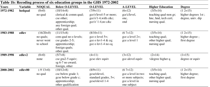
GHS offers two advantages over education measures based on years of schooling. First, the qualification variables outperform schooling years in standard human capital equations (Schmitt, 1991). Second, the value of different types of qualifications, particularly vocational as opposed to academic qualifications, may shed new light on the workings of the supply and demand for skills than an undifferentiated schooling-year variable. In order to simplify the complicated structure of British qualifications, all highest qualifications earned by the respondent are categorized into six groups: NOQUAL, BOLEV, OLEV, ALEV, HIGHER and DEGREE. The complete list and brief description of education variables are presented in the Table 1a, and the recoding process of six education groups in the GHS 1972-2002 is presented in the Table 1b.
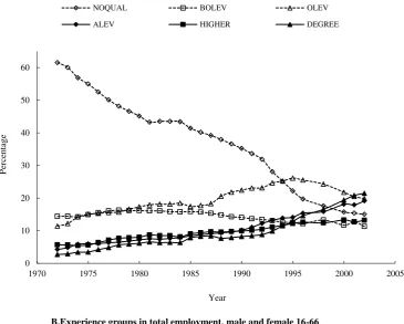
Since 1973, all British children have had to attend full-time education until the age of sixteen. Those who have never gone to school and who have never earned a qualification consist of the group of workers without qualifications (NOQUAL). According to the GHS, NOQUAL was the largest group in the total employment before 1994 (for example, about 61.5 percent in 1972). This group has decreased rapidly over the last thirty years so that only about 15 percent of workers had no qualifications in 2002, as shown in Panel A of Figure 1.
Those who earn qualifications follow either a vocational or an academic track. Following Schmitt (1995), the vocational qualifications increase in skill from miscellaneous, relatively low-skilled apprenticeships (VOC-OTHER) through incremented, nationally recognized apprenticeships (VOC-LOW, VOC-MIDDLE, and VOC-HIGH). The highest level vocational qualifications can involve some instruction at college level.2 School children following the academic track prepare for and sit a series of national tests by academic subject. Those who finally earn the lowest academic (below O-LEVEL) or vocational qualifications (VOC-OTHER) are categorized into the BOLEV group. The BOLEV group also decreased from about 14 percent in 1972 to 11 percent in 2002 in Panel A of Figure 1.
Students passing grades on a series of national tests by academic subject, generally taken around age 16, may earn qualifications that would place individuals in the OLEVEL 1-4, O-LEV&CLER, and O-LEVEL 5+ categories. The “Ordinary
Level” examination categories distinguish between students who pass between one
and four examinations, and those who attempt and pass five or more. The distinction is important for some employers and for further study. Workers with these O-LEVEL equivalent or VOC-LOW qualifications are categorized into the OLEV group, which increased from about 10 percent in 1972 to about 20 percent in 2002 in Panel A of Figure 1.
After O-LEVEL, some students (usually around age 18) take further national
examinations at “Advanced level”. For some students, A-LEVEL is a terminal qualification; for others they are only a prerequisite for university admission. Workers with these A-LEVEL equivalent or VOC-MIDDLE qualifications are categorized into the ALEV group. The ALEV group has increased five-fold from about 4 percent to 19 percent over the entire period.
The remaining two education groups have also increased over the last thirty years. The HIGHER group includes college equivalent qualifications, which consist of all educational or professional qualifications below degree level but above GCE
2
A-level (For example, Teaching, Nursing and VOC-HIGH). The employment share of the higher education group (HIGHER, about 10 percent in 2002) has doubled in the last thirty years. The DEGREE group here includes all respondents who successfully finished the standard three-year university course as well as those who study further. In particular, the employment share of the DEGREE group has increased about nine-fold from 2.7 percent to 22 percent over the period 1972-2002. Thus, the employment composition has shifted to a more educated (skilled) structure, revealing the dramatic changes of skill supply in the British labour market.
(Figure 1 around here)
The experience variable is defined in the standard way as the minimum of (age-years of education-5, age-16).3 This assumes that all workers should enter education at the age of five and cannot leave school before they are sixteen years old. Observations are categorized into eight groups, each covering five years of experience. Card and Lemieux (2001) argue that the United Kingdom experienced a baby boom in the 1950s and the falling supply of college graduate in this cohort may raise the earnings returns of college degrees for the young in the 1980s. Daveri and Maliranta (2007) also reveal the impact of age and seniority on wages and productivity in Finland. More British people are staying longer in the workforce so common practice of excluding experience over 40s may be introducing biases. Thus, workers with more than 40-year experience are also put into the last experience group.
In Panel B of Figure 1, the employment share of new entrants (with 0-10 years of experience) was quite stable in the 1970s and decreased from about 25 percent to about 19 percent during the 1980s and early years of the 1990s. At the same time, the employment share of prime experienced workers (with 21-30 years of experience) had continuously increased from about 20 percent to about 27 percent. Just as in other developed countries such as the US and Canada, the evolution of experience structure in Britain reflects a baby boom in the 1950s (Card and Lemieux, 2001) and the long term aging process of the workforce. Thus, higher employment shares of prime experienced workers reflect a slight shift to the more experienced structure in the British labour market.
2.2 Wage variables in the GHS
The wage variable used in this paper is the real gross hourly earnings, deflated by the annual Retail Price Index (RPI) with 1995 as 100. This deflating factor is calculated from the prices of all items excluding mortgage interest payments provided by the Office for National Statistics (ONS). The wage variable is from a wage sample including all full-time employees aged sixteen to sixty-six.“Full time employee” here is defined as workers (excluding employer and self-employed) with weekly working hours exceeding 35 hours. Self-employed workers, part time workers and those working without pay are excluded from the sample. Our variables for earnings are all calculated from the wage sample which provides accurate wage information and exclude extreme cases of earnings.
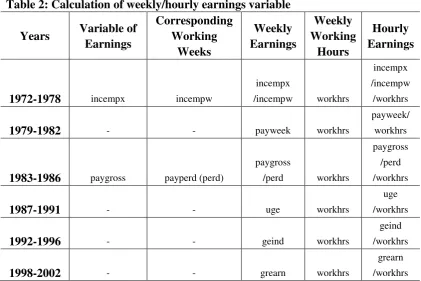
(Table 2 around here)
3
The complete list and a description of the earnings variables are presented in Table 2. This hourly wage variable is derived as follows. Firstly, gross earnings before any deduction are divided by the corresponding payment period (weeks). Schmitt (1995) also thinks the real gross weekly wage is the most continuous measure of the unit price of labour input in the GHS. Secondly, real weekly earnings are divided by weekly working hours (workhrs) to calculate real hourly earnings. According to the ONS (2006), before 1996, workhrs gives the “Usual number of hours worked per week excluding mealtime and overtime”. But, after 1996, this variable includes mealtime and overtime. Figure 2 describes changes of the weekly working hours by gender. The left vertical axis represents the mean working hours for all full-time workers, males and females. The right vertical axis represents the working hours gap between males and females. We can find weekly working hours of all three groups are quite stable over the entire period. Full time males work longer time, about 42 hours per week than females (about 39 hours per week). Moreover, the working hours gender gap has been slowly increasing after the 1970s, from about 2 hours in 1980 to about 4 hours in 2002. Since the working hour variable before 1996 does not include over time, our hourly earnings variable may be affected by the different coverage of the weekly earnings variable and working hour variables in the GHS.
(Figure 2 around here)
The main concern about our wage variable is likely to be the measurement of overtime working hours. The overtime working hours are commonly regarded as short-term employment adjustment mechanism that enables firms to meet unexpected variations in demand without incurring the fixed costs of hiring or firing workers (Bils, 1987). Bell et al. (2000) find that a significant number of employees work more hours in the workplace than their contract stipulates. The overtime working is an important part of working hours in the British labour market and the quantitative significance of both paid and unpaid overtime is even greater in the UK (than in Germany).4 The missing overtime problem in weekly working hours may bring upwards biases in the levels of hourly wage rates calculated from weekly earnings divided by weekly working hours as in this paper, which also could bring counter-cyclical biases for the changes of hourly wage over business cycle if the weekly overtime is also counter-cyclical (Peng and Siebert, 2012).
Bell and Hart (2003a) show that without national laws regulating overtime assignment or compensation, British overtime wage premiums are actually independent of overtime hours, and the proportions of overtime workers working at given rates are very similar across the worker groups with different working hours. Moreover, Bell and Hart (2003b) argue that overtime hours and pay are not wholly geared to meet short-term shifts in production requirements even in labour markets like Britain where statutory overtime rules do not apply. The maximum lengths of standard weekly hours set by many firms follow wider industrial or regional or national collective bargaining norms. These observations are consistent with the view
that the conditions for overtime working follow “custom and practice” and a
long-term contractual role for overtime, suggesting that the effect of overtime working in our hourly earnings could be stable over time (Bell and Hart, 2003a).
4
Therefore, the missing overtime in our working hours variable can be regarded a time-invariant factor which would not affect our argument on cyclical changes of wage structure. Hourly wage used in this paper can exclude the cyclical effect of working hours from earnings variable hence be a more accurate measurement than weekly earnings.5
3. Changes in Wage Structure
3.1 Gender gap
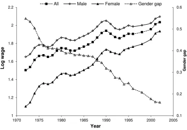
We firstly present a broad empirical characterization of the evolution of the wage structure in the UK during the period 1972-2002. Figure 3 describes changes of the real hourly wages by gender. The left vertical axis represents the log form mean wage for all full time workers, and for males and females. The right vertical axis represents the wage gap between males and females. We can see that over the entire period, the real hourly wage of all full time workers increases by about 60 percent (from 1.46 in 1972 to 2.06 in 2002).6 Since about two thirds of the full time workers are males, the mean wage of males has increased by a similar magnitude as the full work force, that is, 50 percent over the entire period (from 1.61 in 1972 to 2.11 in 2002).
(Figure 3 around here)
At the same time, Figure 3 indicates that the mean wage of females has increased by about 90 percent over the thirty years (from 1.06 in 1972 to 1.96 in 2002). This result suggests that the gender gap between males and females has decreased by about 40 percent (=90-50). In 1972, full time males earned about 55 percent (=1.65-1.10) more than females, while wage gap decreased to less than 40 percent in 1980, and then to only 16 percent (=2.10-1.94) in 2002.7 Since the wage gap between males and females has been decreasing over the last three decades, the narrowing gender gap should decrease overall earnings inequality. Thus, the well documented rising earnings inequality in the UK must be from the worsening inequality within rather than between gender groups.
3.2 Wage inequality within gender group
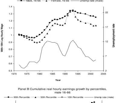
In order to illustrate the rising inequality within each gender group, Panel A of Figure 4 summarizes movements of wage inequality by gender. It plots the times series of wage inequality for males and females measured as the log wage differentials between the ninetieth and the tenth percentiles of the wage distribution. Overall hourly wage inequality (90th-10th percentile differentials) has increased by about 25 percent (from about 1.0 in 1972 to about 1.25 in 2002) for males as well as by about 13 percent
5
The main conclusions do not change as we test the sensitivity of our results by replacing hourly wage with weekly earnings. In particular, the cyclical patterns of labour demand are still prominent using weekly earnings. It suggests that the overtime part of the weekly working hours be time-invariant (or rigid) as discussed in Bell and Hart (2003a, 2003b).
6
We refer to 100 times log changes as percentage changes.
7
GHS oversampled married women in the early years so reduction in the wage gap might also reflect this sampling bias. The GHS Summary Quality Report from ONS (2007a) also admits: “one of the limitations of the GHS is that the nature of the sample design means that the precision of survey estimates is reduced ……Although this effect is reduced by the use of stratification it is nevertheless a
(from about 1.0 in 1972 to about 1.13 in 2002) for females over the entire period. Moreover, with this long term increasing trend, wage inequality in the UK follows a cyclical pattern over the entire period. The figure shows earnings inequality narrowed in the 1970s, especially for females, and moved up until the early years of the 1990s. After 1995, the rising trend of earnings inequality was definitely reduced for females and kept quite stable for males. This graph is consistent with results of Prasad (2002).
We use the national unemployment rate of males as an indicator of business cycle, which is derived from the Labour Force Survey (LFS) (ONS, 2007b). Panel A of Figure 4 shows that the earnings inequality increases as the labour market becomes loose, vice versa. It suggests that the earnings inequality would increase with increasing unemployment rates, as well as decrease with decreasing unemployment rates. This counter-cyclical phenomenon is even more prominent for females than for males. Barlevy and Tsiddon (2006) find the similar counter-cyclical pattern of earnings inequality using data of the first half of the 20th century. They argue that recessions should contribute more to raising inequality when inequality is rising over the long run than when it is falling. During the 1970s and years after mid-1990s, we find the increasing unemployment (recession) has no much effect on the falling inequality. However, during the 1980s and early years of 1990s, the rising inequality is more sensitive to the recessions. Our findings in Panel A are consistent with their model.
(Figure 4 around here)
Barlevy and Tsiddon (2006) also point out that cyclical fluctuation affects workers at different locations of earnings distribution in different ways, and ultimately shaping the distribution of earnings over the business cycle. Panel B of Figure 4 illustrates this image by plotting the cumulative log real wage growth of three groups - the tenth, fiftieth, and ninetieth percentiles of the wage distribution - for males. More precisely, the figure displays the log ratio of each group’s real hourly earnings in each
year relative to that group’s level of real earnings in 1972 (the baseline year), and gives us a snapshot of the movement in earnings of the three groups.
In Panel B of Figure 4, recessions in business cycle correspond to periods of rising unemployment and dropping wages, so all three groups show procyclical wages, in line with micro evidence from the past thirty years of the UK (Devereux and Hart, 2006; Devereux and Hart, 2007; Peng and Siebert, 2012) and the USA (Shin and Solon, 2007). However, wages of the top percentile group are more sensitive to the recovery of business cycle and increase much faster than the middle and bottom percentile group during the 1980s and early years of the 1990s. Wages of the poor group have achieved the least growth (only about 42 percent) among the three groups over the entire period, and then the middle group (about 48 percent), while the wages of the rich group have grown fastest (about 62 percent). Hence, the rich have grown richer at faster pace than the poor in the last thirty years and ultimately reshape the earnings distribution.
with so many working in finance, there is a strong link between fortunes of the rich group and those of the stock market. Similarly, the graph of the 90th percentile in Panel B maintained high speed over the entire period, maybe due to the ICT booming in production (O'Mahony et al., 2008) and the “dot-com bubble” in financial market covering roughly 1995–2001 (Goldfarb et al., 2007). Hence, wage of the rich group is not only following a long term increasing trend but also highly procyclical to business fluctuation.
Wages of the middle and poor groups also show overall procyclical pattern over time. However, wages of the poor group are not so sensitive as the middle and rich groups to the business recovery around the mid-1980s. Hence, wages of the poor group had been left behind further by the other two groups during the big unemployment shock around the mid-1980s. With the decline of trade union’s collective bargaining (Blanchflower and Bryson, 2010), wages of the poor group become more sensitive to business cycle during the 1990s and the 2000s and increase very fast after the unemployment shock of the mid-1990s. This time, it is wages of the middle group that are sticky and insensitive to the business recovery. This result is
consistent with the findings of O’Mahony et al. (2008) that the intermediate skill groups became more disadvantageous in the 1990s than in the 1980s. O’Mahony et al. (2008) also find an increasing complementarity between capital and unskilled labour in the 1990s. Thus, with help of better adaptation for technology in the 1990s, the earnings of the poor group converged to the middle group quickly over the last years in our sample.
4. A standard earnings equation
4.1 Evolution of the skill premium
Next, we apply a standard earnings equation to do repeated cross-section regressions. Workers’ educational qualifications and experience are used as skill proxies to analyse the evolution of skill premiums over time. Moreover, we also estimate residual wages after these repeated cross-section regressions. Residual wage inequality is the dispersion of wages after controlling for the measured supply-demand changes of skill groups. Thus, residual inequality is the part of overall inequality unexplained by measurable skill variables such as education and experience.
Hourly earnings are estimated for males and females in a repeated cross-section regression as in Katz et al. (1995):
lnwi = a + b1Qi + b2 Expi + b3 Expi2 + b4Ri +b5Wi+b6Mi +b7 Tt +ei (1)
The dependent variable lnwi is log form real gross hourly pay. Explanatory variables include a vector of five education dummies Qi: BOLEV, OLEV, ALEV, HIGHER and DEGREE (NOQUAL as the baseline group); the quadratic experience terms (Exp and Exp2) to capture the concavity of the experience earnings profile, a vector of four region dummies Ri: MIDLAND, SOUTH, WALES and SCOTLAND (Northern England as the baseline group), an ethnicity dummy set as 1 for white people (Wi), a marital status dummy set as 1 married people (Mi) and a vector of year dummies Tt only for pooled datasets; ei is an error term.
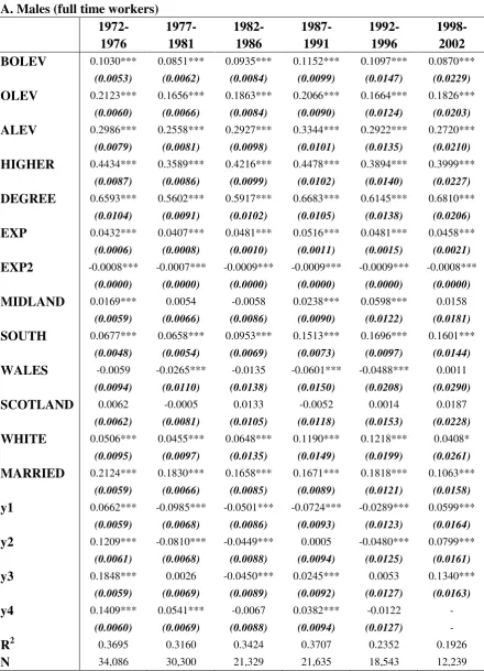
premiums for both males and females in each period. For instance, during the period 1998-2002, males in the DEGREE group earn about 68.1 percent more than males in the NOQUAL group, while males in the BOLEV group only earn about 8.7 percent more than the NOQUAL group. The highest return from education is for the DEGREE group, which is about 30 percent higher than the second highest educated group (HIGHER) for both males and females. Hence, more education brings higher earnings. And, degrees from university are the most important education qualification for earnings. This result is consistent with the considerable existing literature on education return e.g. Harmon, Hogan and Walker Harmon et al. (2003b), Harmon, Oosterbeek and Walker (2003a) and Walker and Zhu (2003; 2005).8
Education premiums in Table 3 have shown a cyclical pattern with an increasing trend over the entire period for males, but this increasing trend is more evident after the 1970s.9 Moreover, the more educated are male workers, the faster do their education premiums grow after the 1970s. This clear ranking in education premium growth after the 1970s is as follows: 12.1 percent for DEGREE (=0.681-0.560), 4.1 percent for HIGHER (=0.4-0.359), about 2 percent for ALEV and OLEV, and no much change for BOLEV. Those males who are more educated seem to have faster wage growth. Consequently, the more dispersed education premiums have pushed up male wage inequality since the 1970s.
Females in Table 3 also show that the large earnings premium is associated with more education. And, education premiums of females are higher than those of males (Walker and Zhu, 2003). However, females’ education premiums are more stable and cyclical than males. And, primary education (BOLEV and OLEV) are much
more important for females’ earnings than for males’. For example, wages of females
in the BOLEV group have increased by about 3.08 percent (=0.1517-0.1208) as well as about 5 percent (=0.228-0.1822) in the OLEV group since the 1970s. Earnings premiums of higher educated groups (ALEV, HIGHER and DEGREE) have not changed much over the entire period.
Therefore, we find the earnings premiums of all education groups have been increasing, at least stable after the 1970s for both males and females. With recent rapid expansion of high education (see Figure 1), our results suggest that the increased supply of graduates has been absorbed by the labour market, implying that the demand for skills has overwhelmed the supply of skills, at least increased roughly in tandem in recent two decades. Our findings are consistent with Harmon, Hogan and Walker (2003b) and Walker and Zhu (2005) using different data sources.
The coefficients of quadratic experience are reported in the next four rows in Table 3. Similar to education premiums, there is also an increasing trend of the experience premiums for both males and females over the entire period (especially
after the 1970s). Moreover, the females’ experience premiums increase much faster
than males’. As can be seen, the experience premiums of females increase from 3.56
percent in the period 1972-1976 to 4.59 percent in the period 1998-2002, while the experience premiums of males only increase from 4.32 to 4.58 percent.
8
For example, Walker and Zhu (2003) demonstrate, mainly using the Labour Force Survey (LFS), that there is a large earnings premium associated with more education – perhaps as much as 10 per cent per additional year of education.
9
Considering the quadratic effect of experience, and controlling for other variables, a female worker with 10 years of experience would earn about 28.6 percent (=3.56×10-0.07×100) more than a new entrant in the period 1972-1976, while she would earn about 36.9 percent (=4.59×10-0.09×100) more in the period 1998-2002. However, there is no such dramatic increase in the experience premiums of males. Thus, the experience premiums of females have grown faster than males and become similar to males in recent years.
(Table 3 around here)
Our regressions also show some other points worthy of mention. Firstly, regional premium is only prominent for the south of England (including the Great London area), which increases from 6.77 percent to 16.01 percent for males, and from 11.56 percent to 16.43 percent for females over the last thirty years. For other regions, there is no continuous significant regional premium compared with the north of England. Hence, only the south of England (including the Great London area) is different from other regions and the wage gap between the south of England and others is becoming wider, showing it is becoming the most prosperous area in the UK.
Secondly, ethnicity is important for males but not for females (especially in the 1970s and 1980s). Married males earn more than unmarried, while married females may earn a little less, but not significant. Obviously, these control variables contribute little to changes of wage structure (and the increasing earnings inequality). The main measurable variables to explain the higher earnings inequality are skills, i.e. education attainment and its earnings premium (Gosling et al., 2000; Harmon et al., 2003a).
Finally, R-squared values in Table 3 decrease from 36.95 percent in 1972-76 to 19.26 percent in 1998-2002 for males. Much literature also shows that measured characteristics (gender, education and experience) of workers can only explain about thirty percent of wage variations (Katz et al., 1995). The declining explanatory power of measured characteristics may reflect the inaccuracy of educational qualifications as an approximation of human capital. For instance, Nickell and Bell (1996) argue that primary education quality in the UK has declined, which may decrease the explanatory power of primary education. Since educational qualifications are imperfect proxies of human capital, wage variations from policy changes or other unmeasured characteristics such as ability or education quality are reflected in the residuals of equation (1).
4.2 Residual wage inequality
We now do the repeated cross-section regressions for each year. After controlling for the characteristics of workers, the distribution of residuals from these regressions may be thought of as capturing the dispersion of wage unexplained by the supply and demand framework. The Panel A of Figure 5 plots the 90th-10th percentile differentials of residual earnings for males and females and shows a very similar cyclical pattern to the overall inequality in Figure 4. The recessions around the 1980s and 1990s would contribute to raising residual inequality, while the recovery around the year of 1990 and the 2000s dramatically decrease residual inequality. Our results show that, after controlling for skills (and their cyclicality), residual inequality is still affected by business cycle.
distribution to show no tendency toward greater inequality. The overall inequality would only stem from changing skill endowments or market valuations of human capital that the earnings regressions would remove from the data (Schmitt, 1995). The Panel A of Figure 5 seems supportive to Schmitt (1995)’s argument. For example, the residual inequality of females only shows a cyclical movement without tendency toward greater inequality over the entire period (around 0.9 in 1972 and 2002). During which the overall inequality has increased by 13 percent over the same period (see Panel A of Figure 4). Hence, changes in the skill endowments and market valuation can fully account for the changes in female earnings inequality over the entire period. For males, the residual inequality has increased by only 14 percent from 1972 (0.83) to 2002 (0.97), compared with 25 percent in the overall inequality (from about 1.0 in 1972 to about 1.25 in 2002, see Panel A of Figure 4). By this crude measure, changes in the skill endowments and market valuation can account for about 44 percent i.e. (25-14)/25 of the changes in male earnings inequality over the entire period. Hence, for males, approximately 56 percent (=14/25) of the increase of overall earnings inequality has occurred within education and experience groups. This result is very similar to Schmitt (1995) who claims that about 60 percent of the increase of earnings inequality occurred within education and experience groups in the period 1978-1988. Therefore, the residual inequality of males shows a cyclical movement with a much less increasing tendency toward greater inequality over the entire period.10
(Figure 5 around here)
Panel B of Figure 5 plots the cumulative growth of the tenth, fiftieth, and
ninetieth percentiles of males’ residual wage. The residual wages of three groups show different sensitiveness to shocks from business cycle, which decides the evolution of residual wage inequality. Firstly, the residual wages of the middle group (or semi-skilled workers) are quite stable around zero and insensitive to shocks from business cycle before 1990. Furthermore, the jump of residual wages around the mid-1990s even shows a counter-cyclical pattern, which may be associated with disadvantage of semi-skilled workers in capital complementarity in the 1990s (O'Mahony et al., 2008). Hence, compared with the middle group in Figure 4, wage procyclicality with the increasing trend of the middle group has been represented by changes in skill endowments and market valuation.
Secondly, the residual wages of the poor group are also quite stable around zero and insensitive to business cycle during the 1970s and the 1980s. However, after 1990, their residual wages show high procyclicality and become very sensitive to the recovery of business cycle. Hence, the tenth percentile of residual wages increases very fast and quickly converges to the middle group in the last ten years of our sample.
10
This result is consistent with O’Mahony et al. (2008) which find an increasing complementarity between capital and unskilled labour in the 1990s.
Finally, the residual wages of the rich group only show an increasing trend without clear cyclicality. Hence, the 90th-50th percentile differentials of residual wages have been increasing after the 1970s. Compared with the rich group in Figure 2.4, wage procyclicality and its partial increasing trend of the rich group have been represented by changes in skill endowments and market valuation. Thus, the increasing residual wage inequality of males is mainly from the increasing trend of the rich group, which cannot be explained by changes in skill endowments and premiums.
5. Conclusions
Through a standard earnings equation, we do repeated cross-section regressions for real wages of males and females. We find that the overall real hourly wage has increased by about 60 percent in the UK from 1972 to 2002. Gender premiums have been decreasing over the last thirty years. Wages of females increase by 40 percent relative to the wages of males. Although narrowing gender gap is good for alleviation of wage inequality, wage inequality within gender group have been increasing. Overall hourly wage inequality (90th-10th percentile differentials) increased by about 25 percent for males as well as by about 13 percent for females over the entire period.
Moreover, wage inequality shows a cyclical pattern, which may be from the different wage cyclicality of the top, middle and bottom percentile groups. These changes of wage inequality can be explained by the changes of skill (education and experience) premiums. The education premiums of males also show a cyclical pattern with somewhat increasing trend, especially after the 1970s. Higher educated male workers have experienced a faster growth of the education premiums so that the wages of males have become more dispersed after the 1970s. However, female workers with only primary education have faster wage growth than higher educated ones. Moreover, the experience premiums of females have grown faster than males and become similar to males in recent years.
Figure 1: Relative skill shares in total employment
Sources: General Household Surveys 1972-2002. All numbers are from the males and females aged 16-66. Except the first and last years (1972 and 2002), all points are three-year averages.
0 10 20 30 40 50 60
1970 1975 1980 1985 1990 1995 2000 2005
P
erc
en
tag
e
Year
A.Education groups in total employment, male and female 16-66
NOQUAL BOLEV OLEV
ALEV HIGHER DEGREE
17 19 21 23 25 27
1970 1975 1980 1985 1990 1995 2000 2005
P
er
ce
n
ta
g
e
Year
B.Experience groups in total employment, male and female 16-66
Figure 2: Mean working hours changes by gender, GHS 1972-2002
Sources: General Household Surveys 1972-2002. All numbers are from the full-time workers aged 16-66 (workhrs>35). Except the first and last years (1972 and 2002), all points are three-year averages.
Figure 3: Mean wage changes by gender, GHS 1972-2002
Note: The numbers in the figure represent log hourly wages using data from the General Household Surveys, 1972-2002. Wage samples include full-time workers aged 16-66 years who were not self-employed and all earnings numbers are deflated based on 1995 pounds. Except the first and last years (1972 and 2002), all points are three-year averages.
30 32 34 36 38 40 42 44 46 48 50
1970 1975 1980 1985 1990 1995 2000 2005
Year W ee kl y w o rk in g h o u rs 1.5 2 2.5 3 3.5 4 4.5 5 G e n d e r g a p
All Male Female Gender gap
0.1 0.2 0.3 0.4 0.5 0.6 1 1.2 1.4 1.6 1.8 2 2.2
1970 1975 1980 1985 1990 1995 2000 2005
Ge nder gap L o g w age Year
[image:16.595.98.486.440.709.2]Figure 4: Wage inequalities in the UK, GHS 1972-2002
Note: The numbers in the figure represent log changes in hourly wages using data from the General Household Surveys, 1972-2002. Wage samples include full-time workers aged 16-66 years who were not self-employed and all earnings numbers are deflated based on 1995 pounds. Except the first and last years (1972 and 2002), all points are three-year averages.
Panel A Changes in hourly earnings inequality by gender
0.5 0.6 0.7 0.8 0.9 1 1.1 1.2 1.3 1.4
1970 1975 1980 1985 1990 1995 2000 2005
Year 90 th -1 0t h L o g H o u rl y W ag e 2 7 12 17 22 U ne m pl oy m ent r at e
Male, 16-66 Female, 16-66 Unemp rate (male)
Panel B Cumulative real hourly earnings growth by percentiles, male 16-66 -0.5 -0.3 -0.1 0.1 0.3 0.5
1970 1975 1980 1985 1990 1995 2000 2005
Year L o g R ea l H o u rl y W ag e 2 7 12 17 22 U n em p lo ym en t R at e
Figure 5: Residual wage inequalities in the UK, GHS 1972-2002
Note: The numbers in the figure represent log changes in hourly wages using data from the General Household Surveys, 1972-2002. Wage samples include full-time workers aged 16-66 years who were not self-employed and all earnings numbers are deflated based on 1995 pounds. Except the first and last years (1972 and 2002), all points are three-year averages.
Panel A Changes in residual hourly earnings inequality by gender
0.4 0.5 0.6 0.7 0.8 0.9 1 1.1
1970 1975 1980 1985 1990 1995 2000 2005
Year 90 th -1 0t h L o g H o u rl y W ag e 2 7 12 17 22 U ne m pl oy m ent r at e
Male, 16-66 Fem ale, 16-66 Unem p rate (male)
Panel B Cumulative residual real hourly earnings growth by percentiles, male 16-66 -0.5 -0.4 -0.3 -0.2 -0.1 0 0.1 0.2
1970 1975 1980 1985 1990 1995 2000 2005
Year L o g R e a l H o u rl y W a g e 2 7 12 17 22
Table 1a: Education qualification variables in the GHS 1972-2002
Variable Description
NOQUAL NOQUAL includes: Without any qualification or never attended school.
Below O-LEVEL
Below O-LEVEL includes:
CLERICAL: Commerce and clerical qualification without O-levels;
OTHER : CSE grade 2-5 and CSE below grade 1, GCSE below grade c, O-level degraded, SCE degraded, plus all remaining qualifications, which consist mainly of local or regional school-leaving certificates and college or professional awards
no regarded as “ higher educational”, i.e. not above GCE A-level or O-level standard;
FOREIGN: foreign qualification; etc.
VOC-OTHER: Miscellaneous apprenticeships;
O-LEVEL O-LEVEL includes:
O-LEVEL 5+ and equivalent: Five or more subjects at GCE O-level obtained before 1975 or in grades A-C if obtained later, five or more subjects at SCE Ordinary obtained before 1973 or in bands A-C if obtained later, five or more subjects at CSE grade 1 or at School Certificate, SLC Lower, or SUPE Lower;
O-LEVEL 1-4 and equivalent: Less than five O-LEVELS with or without clerical or commercial qualification such as typing, shorthand, bookkeeping, commerce etc;
VOC-LOW: City and Guilds Craft or Ordinary etc;
A-LEVEL A-LEVEL and equivalent includes: GCE A-level in one, two or more subjects,
Scottish Leaving Certificate (SLC), Scottish Certificate of Education (SCE), Scottish University Preliminary Examination (SUPE) at Higher Grade, Certificate of Sixth Year Studies;
VOC-MIDDLE:
City and Guilds Advanced or Final, Ordinary National Certificate (ONC) or Diploma (OND), BEC/TEC National, General, or Ordinary etc.
HIGHER EDUCATION
HIGHER EDUCATION includes:
TEACHING: Non-graduate teaching qualifications (Census Level C);
NURSING: Nursing qualifications (e.g. SEN,SRN,SCM);
VOC-HIGH:
HND and equivalent: Higher National Diploma [HND]/Higher National Certificate [HNC], BEC/TEC Higher Certificate or Higher Diploma; City and Guilds Full Technological Certificate, qualifications obtained from colleges of further education or from professional institutions below degree level but above GCE A-level standard
DEGREE DEGREE includes:
Table 1b: Recoding process of six education groups in the GHS 1972-2002
Years Variable NOQUAL Below O-LEVEL O-LEVEL A-LEVEL Higher Education Degree
1972-1982 hedqual (0=0) (10/14=8) (7/9=11) (6=12) (3/5=14) (1 2=15)
no qual clerical & comm qual; cse other;
apprenticeship; any foreign qual; other qual.
gce'o'level-5 or more; gce'o'1-4,with c&c; gce'o' 1-4,no c&c
gce'a'level, onc, ond
teaching qual-non gr; hnc, hnd, tech cert; nursing qual.
higher degrees 1st ; degree, univ. dip
1983-1988 edlev (16/20=0) (11/15=8) (8/10=11) (6 7=12) (3/5=14) (1 2=15)
no quals; never went to school
com qual no o levels; cse grades 2-5;
apprenticeship; foreign quals; other qual.
gce o level 5+; gce o lev1-4 & cq; gce o lev1-4 no cq
gce a level 2+; gce a level 1
teaching qual; other higher qual; nursing qual
higher degree ; first degree
1989-1998 edlev2 (8=0) (5/7=8) (4=11) (3=12) (2=14) (1=15)
none cse gra2-5 equiv; sg 6-7 no award; foreign, other
gcse olev equiv gce alevel equiv <degree higher q degree or equiv
2000-2002 edlev00 (-9 13=0) (10/12=8) (8/9=11) (6 7=12) (3/5=14) (1 2=15)
no qual cse below grade 1; gcse below grade c; apprenticeship; other qualification
gcse/olevel, standard grades, 5+; gcse/olevel 1-4
gce a level in two or more subjects; gce a level in one subject
teaching qual; other higher qual; nursing qual
higher degree; first degree
Sources: The General Household Survey 1972-2002.
Table 2: Calculation of weekly/hourly earnings variable
Years Variable of Earnings
Corresponding Working
Weeks
Weekly Earnings
Weekly Working
Hours
Hourly Earnings
1972-1978 incempx incempw
incempx
/incempw workhrs
incempx /incempw
/workhrs
1979-1982 - - payweek workhrs
payweek/ workhrs
1983-1986 paygross payperd (perd)
paygross
/perd workhrs
paygross /perd /workhrs
1987-1991 - - uge workhrs
uge /workhrs
1992-1996 - - geind workhrs
geind /workhrs
1998-2002 - - grearn workhrs
grearn /workhrs Sources: Code manuals of the General Household Surveys 1972-2002 (ONS, 2004).
Note: Definition of earnings variables in the GHS: Incempx: Gross income from employment in last year. Incempw: No. weeks income from employment in last year.
Workhrs: No. hours worked per week in main job -excluding meals and overtime. Payweek: Gross weekly earnings from main job.
Paygross: Gross pay of last time from main job before any deduction.
Payperd (perd): Period covered by last wage or salaries, which is corresponding working weeks of paygross11.
Uge: Usual gross weekly earnings from main job and other jobs. Geind: Usual gross weekly earnings from main job and second job. Grearn: Gross weekly earned income from main job and second job.
For years 1972-1978, weekly earnings were derived from all earnings including wages, salaries, tips, bonus and commissions in all jobs held in the previous twelve months. For years 1979-1986, weekly earnings were estimated as the usual gross earnings including tips and bonuses per pay period from the
worker’s main job, divided by the usual number of weeks covered in each pay period. In the 1987-2002 surveys, weekly earnings include all income earned from the main job and other (or second) jobs. These changes may affect comparisons of earnings between different two periods, but no evident discontinuity is found. On the other hand, weekly earnings include payments for bonuses and overtime but the measurement of working hours per week excludes overtime which varies across individuals and over the business cycle. That implied that hourly earnings in this paper may suffer upwards bias, though the GHS is still consistent and comparable with the hourly earnings from other datasets.
11 Perd
Table 3: Log Hourly Earnings Equations, GHS 1972-2002. Estimation from equation (1)
A. Males (full time workers)
1972- 1976
1977- 1981
1982- 1986
1987- 1991
1992- 1996
1998- 2002
BOLEV 0.1030*** 0.0851*** 0.0935*** 0.1152*** 0.1097*** 0.0870***
(0.0053) (0.0062) (0.0084) (0.0099) (0.0147) (0.0229)
OLEV 0.2123*** 0.1656*** 0.1863*** 0.2066*** 0.1664*** 0.1826***
(0.0060) (0.0066) (0.0084) (0.0090) (0.0124) (0.0203)
ALEV 0.2986*** 0.2558*** 0.2927*** 0.3344*** 0.2922*** 0.2720***
(0.0079) (0.0081) (0.0098) (0.0101) (0.0135) (0.0210)
HIGHER 0.4434*** 0.3589*** 0.4216*** 0.4478*** 0.3894*** 0.3999***
(0.0087) (0.0086) (0.0099) (0.0102) (0.0140) (0.0227)
DEGREE 0.6593*** 0.5602*** 0.5917*** 0.6683*** 0.6145*** 0.6810***
(0.0104) (0.0091) (0.0102) (0.0105) (0.0138) (0.0206)
EXP 0.0432*** 0.0407*** 0.0481*** 0.0516*** 0.0481*** 0.0458***
(0.0006) (0.0008) (0.0010) (0.0011) (0.0015) (0.0021)
EXP2 -0.0008*** -0.0007*** -0.0009*** -0.0009*** -0.0009*** -0.0008***
(0.0000) (0.0000) (0.0000) (0.0000) (0.0000) (0.0000)
MIDLAND 0.0169*** 0.0054 -0.0058 0.0238*** 0.0598*** 0.0158
(0.0059) (0.0066) (0.0086) (0.0090) (0.0122) (0.0181)
SOUTH 0.0677*** 0.0658*** 0.0953*** 0.1513*** 0.1696*** 0.1601***
(0.0048) (0.0054) (0.0069) (0.0073) (0.0097) (0.0144)
WALES -0.0059 -0.0265*** -0.0135 -0.0601*** -0.0488*** 0.0011
(0.0094) (0.0110) (0.0138) (0.0150) (0.0208) (0.0290)
SCOTLAND 0.0062 -0.0005 0.0133 -0.0052 0.0014 0.0187
(0.0062) (0.0081) (0.0105) (0.0118) (0.0153) (0.0228)
WHITE 0.0506*** 0.0455*** 0.0648*** 0.1190*** 0.1218*** 0.0408*
(0.0095) (0.0097) (0.0135) (0.0149) (0.0199) (0.0261)
MARRIED 0.2124*** 0.1830*** 0.1658*** 0.1671*** 0.1818*** 0.1063***
(0.0059) (0.0066) (0.0085) (0.0089) (0.0121) (0.0158)
y1 0.0662*** -0.0985*** -0.0501*** -0.0724*** -0.0289*** 0.0599***
(0.0059) (0.0068) (0.0086) (0.0093) (0.0123) (0.0164)
y2 0.1209*** -0.0810*** -0.0449*** 0.0005 -0.0480*** 0.0799***
(0.0061) (0.0068) (0.0088) (0.0094) (0.0125) (0.0161)
y3 0.1848*** 0.0026 -0.0450*** 0.0245*** 0.0053 0.1340***
(0.0059) (0.0069) (0.0089) (0.0092) (0.0127) (0.0163)
y4 0.1409*** 0.0541*** -0.0067 0.0382*** -0.0122 -
(0.0060) (0.0069) (0.0088) (0.0094) (0.0127)
-R2 0.3695 0.3160 0.3424 0.3707 0.2352 0.1926
N 34,086 30,300 21,329 21,635 18,543 12,239
Continued
B. Females (full time workers) 1972-
1976
1977- 1981
1982- 1986
1987- 1991
1992- 1996
1998- 2002
BOLEV 0.1525*** 0.1208*** 0.1183*** 0.1460*** 0.1750*** 0.1517***
(0.0098) (0.0105) (0.0135) (0.0134) (0.0193) (0.0299)
OLEV 0.2293*** 0.1822*** 0.2259*** 0.2804*** 0.2392*** 0.2280***
(0.0097) (0.0101) (0.0123) (0.0119) (0.0165) (0.0271)
ALEV 0.3787*** 0.3345*** 0.3551*** 0.4331*** 0.3524*** 0.3326***
(0.0180) (0.0169) (0.0172) (0.0156) (0.0199) (0.0278)
HIGHER 0.4663*** 0.4490*** 0.4834*** 0.5864*** 0.5473*** 0.4588***
(0.0162) (0.0143) (0.0159) (0.0148) (0.0195) (0.0291)
DEGREE 0.7357*** 0.6720*** 0.6690*** 0.7679*** 0.7223*** 0.6799***
(0.0270) (0.0208) (0.0185) (0.0165) (0.0202) (0.0270)
EXP 0.0356*** 0.0341*** 0.0424*** 0.0460*** 0.0447*** 0.0459***
(0.0011) (0.0012) (0.0015) (0.0014) (0.0019) (0.0025)
EXP2 -0.0007*** -0.0006*** -0.0008*** -0.0009*** -0.0009*** -0.0009***
(0.0000) (0.0000) (0.0000) (0.0000) (0.0000) (0.0001)
MIDLAND -0.0156 0.0129 -0.0239* -0.0036 0.0304** 0.0144
(0.0110) (0.0114) (0.0136) (0.0125) (0.0164) (0.0224)
SOUTH 0.1156*** 0.1014*** 0.1247*** 0.1746*** 0.1753*** 0.1643***
(0.0087) (0.0090) (0.0108) (0.0100) (0.0129) (0.0176)
WALES -0.0244 -0.0311* 0.0019 -0.0661*** -0.0467* 0.0180
(0.0173) (0.0181) (0.0226) (0.0206) (0.0268) (0.0349)
SCOTLAND -0.0051 0.0069 0.0075 0.0122 0.0198 0.0524**
(0.0103) (0.0131) (0.0159) (0.0155) (0.0199) (0.0266)
WHITE 0.0218 0.0085 0.0299 0.0194 0.0321 0.0726***
(0.0165) (0.0156) (0.0204) (0.0176) (0.0228) (0.0280)
MARRIED -0.0127 -0.0016 -0.0148 -0.0033 0.0266** -0.0243
(0.0084) (0.0092) (0.0111) (0.0106) (0.0138) (0.0183)
y1 0.0593*** -0.0116 0.0131 0.0679*** -0.0806*** 0.0695***
(0.0105) (0.0114) (0.0135) (0.0127) (0.0163) (0.0200)
y2 0.1569*** 0.0855*** 0.0094 0.1282*** -0.0406*** 0.0949***
(0.0107) (0.0114) (0.0138) (0.0127) (0.0166) (0.0195)
y3 0.2727*** 0.1396*** 0.0310** 0.1394*** -0.0096 0.1534***
(0.0105) (0.0113) (0.0136) (0.0129) (0.0165) (0.0197)
y4 0.2782*** 0.0905*** 0.0312** 0.1286*** 0.0065 -
(0.0106) (0.0114) (0.0137) (0.0128) (0.0165)
-R2 0.2786 0.2360 0.2660 0.3280 0.2136 0.1771
Note: The numbers in the table represent the estimated coefficients and standard errors using the pooled GHS datasets of six periods: 1972-76, 1977-81, 1982-86, 1987-91, 1992-96 and 1998-2002. Samples include full-time workers aged 16-66 years who were not self-employed and all hourly earnings numbers are deflated based on 1995 pounds. The dependent variable is log gross hourly pay. Explanatory variables include a vector of five education dummies (BOLEV, OLEV, ALEV, HIGHER and DEGREE, NOQUAL as the base group), the quadratic in experience (Exp and Exp2), four region dummies (MIDLAND, SOUTH, WALES and SCOTLAND, the North of England as the base group), an ethnicity dummy (WHITE), a marital status dummy (MARRIED) and a vector of year dummies. ***, ** and * denote significance at 1%, 5% and 10% levels for two-tail tests.
References
BARLEVY, G. & TSIDDON, D. 2006. Earnings inequality and the business cycle. European Economic Review, 50, 55-89.
BELL, B. D. & HART, R. A. 2003a. Wages, Hours, and Overtime Premia: Evidence from the British Labor Market. Industrial and Labor Relations Review, 56,
470-480.
BELL, B. D. & HART, R. A. 2003b. How Important Is Guaranteed or Institutionalised Overtime. IZA Discussion Paper No. 766. Bonn: Institute for the Study of Labor.
BELL, D. N. F., HART, R. A., H BLER, O. & SCHWERDT, W. 2000. Paid and Unpaid Overtime Working in Germany and the UK. IZA Discussion Paper No. 133. Bonn: Institute for the Study of Labor.
BERTHOUD, R. 2007. Work-rich and Work-poor: Three decades of change. Produced by The Policy Press for Joseph Rowntree Foundation (ISBN 978 1 86134 954 5).
BILS, M. 1987. The cyclical behavior of marginal cost and priceAmerican Economic Review, 77, 838-855.
BLANCHFLOWER, D. G. & BRYSON, A. 2010. The Wage Impact of Trade Unions in the UK Public and Private Sectors. Economica, 77, 92-109.
BLAU, F. D. & KAHN, L. M. 1996. International Differences in Male Wage Inequality: Institutions versus Market Forces. Journal of Political Economy, 104, 791-837.
BREWER, M., SIBIETA, L. & WREN-LEWIS, L. 2008. Racing away? Income inequality and the evolution of high incomes. IFS Briefing Notes, BN76. CARD, D. & LEMIEUX, T. 2001. Can Falling Supply Explain the Rising Return to
College for Younger Men? A Cohort-Based Analysis. The Quarterly Journal of Economics, May.
DAVERI, F. & MALIRANTA, M. 2007. Age, seniority and labour costs: lessons from the Finnish IT revolution. Economic Policy, January, 117-175.
DEVEREUX, P. J. & HART, R. A. 2007. The Spot Market Matters: Evidence on Implicit Contracts from Britain. Scottish Journal of Political Economy, Special Issue on Labour Contracts and Wages over the Cycle, 54, 661-683. DICKENS, R. 2000. The Evolution of Individual Male Earnings in Great Britain:
1975-95. The Economic Journal, 110 (January), 27-49.
GOLDFARB, B. D., KIRSCH, D. & MILLER, D. A. 2007. Was There Too Little Entry During the Dot Com Era? Journal of Financial Economics, 86, 100-144. GOSLING, A. & LEMIEUX, T. 2001. Labour market reforms and changes in wage inequality in the United Kingdom and the United StatesNBER Working Paper 8413, National Bureau of Economic Research, Inc.
GOSLING, A., MACHIN, S. & MEGHIR, C. 2000. The Changing Distribution of Male Wages in the UK. Review of Economic Studies, 67, 635-666.
HARMON, C., OOSTERBEEK, H. & WALKER, I. 2003a. The Returns to Education: Microeconomics. Journal of Economic Surveys, 17, 115-156.
HARMON, C. P., HOGAN, V. & WALKER, I. 2003b. Dispersion in the Economic Return to Schooling. Labour Economics, 10, 205–214.
KALWIJ, A. S. & ALESSIE, R. 2007. Permanent and Transitory Wage Inequality of British Men, 1975-2001: Year, Age and Cohort Effects. Journal of Applied Econometrics, 22, 1063 - 1093.
KATZ, L. F., LOVEMAN, G. W. & BLANCHFLOWER, D. G. 1995. A comparison of changes in the structure of wage in four countries. In Freeman, R.B. and Katz, L.F. (Eds.) Differences and Changes in Wage Structure, Chicago: University of Chicago Press, 25-67.
KATZ, L. F. & MURPHY, K. M. 1992. Changes in Relative Wages, 1963-1987: Supply and Demand Factors. The Quarterly Journal of Economics, 107,
35-78.
MACDONALD, G. M. 1988. The Economics of Rising Stars. American Economic Review, 78, 155–167.
NICKELL, S. & BELL, B. D. 1996. Changes in the Distribution of Wage and Unemployment in OECD Countries. The American Economic Review, 86,
302-308.
O'MAHONY, M., ROBINSON, C. & VECCHI, M. 2008. The impact of ICT on the demand for skilled labour: A cross-country comparison. Labour Economics, 15, 1435-1450.
ONS 2004. General Household Survey, 2002-2003 [computer file]. Office for National Statistics. Social Survey Division, Colchester, Essex: UK. Data Archive [distributor], July, SN: 4981. Available at:
http://www.esds.ac.uk/government/ghs
ONS 2006. Summary of main topics included in GHS questionnaires: 1971 to 2006. Office for National Statistics.
ONS 2007a. The GHS Summary Quality Report. Office for National Statistics,
ONS 2007b. Labour Market Statistics: unemployment rates by sex and age. Office for National Statistics. http://www.statistics.gov.uk/statbase/TSDdownload2.asp PENG, F. & SIEBERT, W. S. 2012. Real Wage Cyclicality in Germany and the UK:
New Results Using Panel Data. Discussion Paper 2688, Institute for the Study of Labor (IZA), Bonn.
PRASAD, E. S. 2002. Wage inequality in the United Kingdom, 1975-99. IMF Staff Papers, 49, 339-362.
ROSEN, S. 1981. The Economics of Superstars. American Economic Review, LXXI,
845–858.
SCHMITT, J. 1991. Changing returns to education and experience for British males, 1974-88. CEP Working Paper No. 122. Centre for Economic Performance, London School of Economics, Revised April 1992.
SCHMITT, J. 1995. The changing Structure of Male Earnings in Britain, 1974-1988. In Freeman, R.B. and Katz, L.F. (Eds). Differences and Changes in Wage Structure, Chicago: University of Chicago Press, 177-205.
SHIN, D. & SOLON, G. 2007. New Evidence on Real Wage Cyclicality Within Employer-Employee Matches. Scottish Journal of Political Economy, 54,
648-660.
SOLON, G., BARSKY, R. & PARKER, J. A. 1994. Measuring the Cyclicality of Real Wages: How Important Is Composition Bias? Quarterly Journal of Economics, 109, 1-26.
WALKER, I. & ZHU, Y. 2003. Education, Earnings and Productivity: Recent UK Evidence. Labour Market Trends, 111, 145-152.

![arxiv: v1 [math-ph] 25 Jul 2008](data:image/gif;base64,R0lGODlhAQABAIAAAP///wAAACH5BAEAAAAALAAAAAABAAEAAAICRAEAOw==)