An open source simulation platform to support the formulation of housing stock decarbonisation strategies

An open-source simulation platform to support the

formulation of housing stock decarbonisation strategies

Gustavo Sousaa,b,∗, Benjamin M.Jonesb, Parham A.Mirzaeib,

DarrenRobinsona

a

Sheffield School of Architecture, University of Sheffield, S10 2TN

b

Department of Architecture and Built Environment, University of Nottingham, NG7 2RD

Abstract

Housing Stock Energy Models (HSEMs) play a determinant role in the

study of strategies to decarbonise the UK housing stock. Over the past three

decades, a range of national HSEMs have been developed and deployed to

es-timate the energy demand of the 27 million dwellings that comprise the UK

housing stock. However, despite ongoing improvements in the fidelity of both

modelling strategies and calibration data, their longevity, usability and

reli-ability have been compromised by a lack of modularity and openness in the

underlying algorithms and calibration data sets. To address these shortfalls,

a new open and modular platform for the dynamic simulation of national (in

the first instance, the UK) housing stocks has been developed—thehousing

stock Energy Hub (EnHub). This paper describes EnHub’s architecture, its

underlying rationale, the datasets it employs, its current scope, examples of

its application, and plans for its further development. In this we pay

par-ticular attention to the systematic identification of housing archetypes and

their corresponding attributes to represent the stock. The scenarios we

anal-yse in our initial applications of EnHub, based on these archetypes, focus

∗

on improvements to housing fabric, the efficiency of lights and appliances

and of the related behavioural practices of their users. In this we consider a

perfect uptake scenario and a conditional (partial) uptake scenario. Results

from the disaggregation of energy use throughout the stock for the baseline

case and for our scenarios indicate that improvements to solid wall and loft

thermal performance are particularly effective, as are reductions in

infiltra-tion. Improvements in lights and appliances and reductions in the intensity

of their use are largely counteracted by increases in heating demand.

Hous-ing archetypes that offer the greatest potential savHous-ings are apartments and

detached dwellings, owing to their relatively high surface area to volume

ratio; in particular for pre-1919 and inter-war epochs.

Keywords: housing stock, dynamic energy simulation, open-source,

1. Introduction

The UK’s Climate Change Act aims to reduce the 1990 Greenhouse

Gases (GHG) emissions level by 80 % by 2050 [1]. To this end, the Committee

on Climate Change (CCC) has established a series of incremental targets

(or budgets) for the whole energy sector, including the production of 30 %

5

of electricity from renewable sources by 2020, and the reduction of GHG

emissions by 50 % by 2025. The UK emitted a total of 564 MtCO2e in 2011,

which is 36% below the peak value registered in 1979 and 28 % below that

of 1990 [2]. This reduction was mainly caused by a shift from coal to

nat-ural gas, by a displacement of industrial activity (primarily to Asia), and

10

by major improvements in the performance of the transport sector [3]. This

means that even though the reduction in this period is close to the CCC

target, this has largely been achieved in the absence of systematic structural

improvements to reduce energy demands. Some of the more significant

op-portunities for demand reduction are found in the domestic sector, where

15

emissions have been maintained at almost the same level since 1990 [2].

In 2011, the domestic sector contributed 124 MtCO2e to the total

emis-sions; two-fifths of these were caused by the generation of electrical energy

in power stations and the remainder by direct combustion of fossil fuels.

End-use energy demand in the domestic sector is attributed to four key

ser-20

vices: 60% to space heating, 20% to domestic hot water (DHW), 17% to

lighting and appliances, and 3% to cooking [4]. This highlights the

impor-tance of thermal energy flows in the development of Housing Stock Energy

Models (HSEMs).

Efforts have been made to improve the performance of the existing

hous-25

new buildings, serving a larger population, comprised of smaller households.

For this reason, a full understanding of the energy flow in dwellings, and

the factors influencing them, is required to formulate robust policies and

strategies [5, 6] to achieve significant reductions in their carbon emission

30

intensity. This requires further efforts on two fronts. On the one hand,

the disaggregated measurement of end-use energy demand to complement

existing surveys of housing characteristics for a representative sample of

archetypes; and on the other, the formulation and calibration of suitable

HSEMs, describing not only the performance of the existing stock, but also

35

how this stock is likely to evolve in response to policy measures designed to

reduce carbon intensity [7, 8].

In their recent review, Sousa et al. [9] systematically evaluated, using

a detailed matrix characterising their functionalities, usability and

accessi-bility, the attributes of the 29 HSEMs that have hitherto been developed

40

and deployed in the UK. From this they identified the Cambridge Housing

Model (CHM) as being the most fully developed. They also concluded that

a) the models should be transparent so that their underlying algorithms can

be understood and evaluated, and be amenable to improvement; b) future

HSEMs should have a modular architecture so that each module can be

45

edited and additional modules can be added; c) their underlying thermal

models should be dynamic, to support accurate prediction of indoor

tem-peratures and comfort, and the associated operation of heating systems; and

d) databases should track their sources and development, and be

continu-ally updated so they can maintain their validity. Furthermore, a successful

50

dynamic HSEM would ideally capitalise on available computing power, to

support the rigorous and exhaustive testing of alternative decarbonisation

The housing stock Energy Hub (EnHub) platform has been developed

in direct response to these observations. It is open and modular in

struc-55

ture, and enhances the virtues of existing HSEMs by dynamically simulating

the performance of the building archetypes that comprise the UK housing

stock; this latter requiring semantically attributed three-dimensional

rep-resentations. EnHub also facilitates the straightforward testing of targeted

housing stock decarbonisation scenarios, and is readily extensible to support

60

the integration of models predicting household’s investments to reduce their

carbon intensity, and the associated impacts, in response to policies and

strategies designed to stimulate these investments. By dynamically

sim-ulating the stock, it also facilitates the (future) study of how households

apportion the co-benefits arising from these investments: reducing energy

65

use and emissions on the one hand, and improving indoor thermal

com-fort and health on the other. Finally, EnHub improves on computational

scalability using cloud and high performance computing technologies.

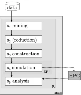
The processing of data to represent the housing stock is achieved using

the statistical computing software R [10]. This is also used to construct

70

dwelling archetypes, which are then simulated using the dynamic building

simulation program EnergyPlus [11]. The platform creates geometrically

simplified models constructed of contiguous cuboids, following the Domestic

Ventilation Model (DOMVENT) [12] and Steadman’s model [13]; assigning

semantic attributes to these cuboids based on survey data (i.e. of envelope

75

properties and household variables). Thus, the platform is able to derive

more informative metrics than has hitherto been possible, including

inci-dences of discomfort, the proportion of the stock that over- or under-heats,

the heat gains per square metre of floor area, the disaggregation of energy

demands, and the estimation of peak thermal and power demands.

The paper begins by describing, in Section 2, the basis of EnHub: its

algorithms and data structures, and the workflow employed in its

applica-tion. Then, in Section 3, a number of scenarios to decarbonise the domestic

stock in the UK are tested and discussed in terms of their effectiveness. The

paper closes by critically evaluating the utility of EnHub, and by identifying

85

how its utility can be further enhanced to support the formulation, and the

more rigorous testing, of alternative decarbonisation policies and strategies.

2. Methods: Statistical Analysis and Engineering Models

The structure of EnHub takes its inspiration from the CHM, which is

at the core of theEnergy Consumption in the UK study [4], and has been

90

identified as the most flexible and powerful of prior HSEMs [9]. The principle

data set underpinning both EnHub and CHM is derived from the English

Housing Survey (EHS), which comprised 14,951 dwellings in its 2011 version,

and is weighted to represent the 21 million houses in England. This data

set is augmented by the Census and the Home Energy Efficiency Database.

95

The principle differences between EnHub and CHM, besides the more

granular and transparent architecture of EnHub, are that:

i. EnHub utilises the dynamic simulation programEnergyPlusfor energy

performance predictions, while CHM uses the Building Research

Es-tablishment Domestic Energy Model (BREDEM), a simplified energy

100

balance model.

ii. EnHub represents dwellings volumetrically, thus explicitly representing

built form and adjacency (e.g. exposed or shared walls), and facilitating

only scales the dwelling archetypes, limiting the analysis of envelope

105

transfers.

iii. EnHub’s archetypes represent the housing stock in a structured

hierar-chical way, which eases communication with its underlying data sets and

facilitates convenient testing of modifications to their attributes, while

CHM requires direct manipulation of models corresponding to individual

110

EHS entries: testing modifications is far from convenient.

iv. EnHub’s architecture is readily extensible to model households’ responses

to socio-economic drivers influencing investments and changes to

be-havioural practice that impact on net building energy demand.

v. EnHub employs a process of statistical data reduction to reduce the

115

number of archetypes to simulate, while CHM evaluates every instance

of the EHS data sets, with corresponding redundancy.

[Figure 1 about here.]

The steps involved in the application of EnHub are conceptually

sum-marised in Figure 1 and are described in detail in the following sub-sections.

120

Once the main data set is integrated into the platform, the open-source

sta-tistical computing platformRis used to mine these data and to reduce the

sample size by determining the most relevant archetypes contained in the

original data set. Then, this reduced data set is re-weighted to match the

original totals. The next step uses the archetypes to create a set of

seman-125

tically enriched volumetric models that are used byEnergyPlusto simulate

dynamic energy flows.

It is worth noting that both R and EnergyPlus can be paired with a

run in Command Language Interface (CLI) mode. In this way, both can

130

be controlled from within a shell1. The purpose of using a shell is that

1) the platform can be detached from the operating system and 2) a set

of low-level scripts can systematically control the modelling process. This

enables parallelisation, so that a High Performance Computing (HPC)

fa-cility can be called upon to accelerate the computation tasks, by around

135

two orders of magnitude. In this way, a number of computer nodes can be

simultaneously requested, each being allocated an instance of EnergyPlus

and a corresponding EnergyPlus Input Data File (idf). Hence, the

paralleli-sation of the simulation process depends on available HPC resources. The

generated data, on any chosen hardware, can then be re-integrated into the

140

process described in Figure 1. The results are then extrapolated to the

sub-sets of the UK stock represented by these archetypes, and the results are

analysed.

2.1. Step 1: Data Mining

To provide a level of confidence in the EHS data set, a data mining

pro-145

cess is performed. Data mining involves the application of diverse methods

to predict and/or classify typically complex databases [14, 15]. Predictive

methods usually apply regressions, although a highly developed sub-type

in-cludes hierarchical models (e.g. trees, additive models, neural networks) [5].

Classification methods usually apply cluster and ordination analyses, and

150

are mainly used to study large databases. Both predictive and classification

methods identify the proximity2 between variables, and can be adapted and

1

A shell is a program which provides an interface between the user and the operating system. Such an interface may be called via a CLI or via scripting files.

2

complemented to obtain further information about their emerging

relation-ships. For example, the strength of correlation between a range of input

variables and an output may determine influential input parameters; some

155

input variables may have a similar influence on the output, so they can be

combined or classified to reduce repetition. In studies employing survey

data, it is common to interpret a variable as an independent predictor (also

known as model misspecification), whereas in reality this should be linked

to functional associations. Looking at both the origin of the data and the

160

units of observation helps to identify such associations.

For housing stock studies, the chosen units of observation may be

di-rectly derived from real archetypes (representative samples) or deployed as

average archetypes (synthetic samples) [16, 17, 18, 19]. Their selection

de-pends on both the purpose of the study and the developer’s expertise. The

165

formation of archetypes requires predictive methods to define associations,

and to derive fit-for-purpose units of the stock. It is possible to use both

techniques to incorporate multiple sources of information, and to enhance

the robustness of the archetypes.

When considering a data set with inputs and outputs, the first step is

170

to test its linearity (summarised in the upper part of Algorithm 1). This is

useful for revealing similarity in the inputs, statistical independence of the

output variables, and—for the case of multiple variables—clusters of data.

To this end, two parameters are essential to define the level of linearity

among variables: proximity and correlation coefficients. Depending on the

175

structure of the data set (i.e. types of variables, number of cases, weights,

survey design), both parameters can be employed to ensure that reduced

versions of the dataset are appropriately structured and scaled. Previous

association [20, 21, 22], and there appears to be agreement in the value of

180

employing robust methods to account for the influence of categories, and

more importantly, to identify redundant variables in terms of their level of

significance [5, 23]. Robust methods apply criteria to reduce the impact of

multicollinearity, partial effects, and unclear distributions [24]; for instance,

by employing median values to identify influential variables, by removing

185

outliers, or by assuming partial distributions to avoid misleading tendencies.

Algorithm 1Data mining (on top) and reduction (on bottom) processes. Notation: ←

meansassigned from;→meansassigned to;∝meansis proportional to; := meanscreates and assigns

1. t e s t for l i n e a r i t y

L←glm(EHS, OutEnHubEnergySimulation)

190

2. t e s t for c o r r e l a t i o n

C←f pca(EHS, OutEnHubEnergySimulation)

3. s e a r c h for r e d u n d a n c y a p p l y i n g b a c k w a r d s e l i m i n a t i o n

glm(L, C, OutEnHubEnergySimulation)backwards

195

-4. re - s a m p l i n g p r o c e s s b a s e d on m i n i n g o u t c o m e s EHSreduced←(EHS∝LHS(EHS))

200

5. kruskal - w a l l i s t e s t and c o m p a r i s o n for c o n s i s t e n c y

KW t(EHS, EHSreduced)

6. o b t a i n p o p u l a t i o n s u b t o t a l s , i . e . the a c c u m u l a t e d

205

sum for e a c h g r o u p ( n )

TP →S1+S2+...+Sn

7. o b t a i n s a m p l e s u b t o t a l s Ts→s1+s2+...+sn

210

8. c o m p e n s a t e w i t h s c a l i n g f a c t o r for e a c h v a r i a b l e

cn→Sn/sn

9. a d j u s t p a r a m e t e r s a c c o r d i n g l y ( m e d i a n s or m o d e s )

215

if n:numeric t h e n si:=Se_i

if n:categorical t h e n si:=Sbi

10. re - c o n s t r u c t s a m p l e u s i n g the c o m p e n s a t e d f a c t o r s Ts0→s1·c1+s2·c2+...+sn·cn

220

In our case, a linearity test is performed via Focused Principal

to identifying potential overlaps among the variables. FPCA extends the

classic approach of Principal Component Analysis (PCA) that applies scores

225

to the variance of the data and, by extracting the proximity of those

vari-ables that are ranked most highly, identifies redundant varivari-ables. It is also

useful in testing for correlations between variables, the presence of clusters,

and the measurement of variability [25] and collinearity [26]. FPCA is used

because it provides a virtual rank of the variables, thus identifying those that

230

are most influential. Furthermore, because non-linear relations and mixed

effects are expected in the EHS, FPCA is useful in ranking variables that

include categorical variables; acknowledging that, due to the dimensions of

the EHS, the outcomes are merely indicative and should be complemented

with alternative methods.

235

To tackle the problem of multicollinearity, GLMs may also be applied

to eliminate redundant variables. GLMs extend ordinary linear models by

including a distribution of the expected response and by assuming that more

than one variable is dependent [27]. In this way, as with FPCA, GLMs rank

the variance in the variables in addition of the level of significance3.

240

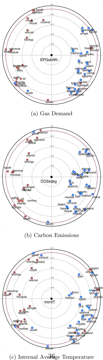
[Figure 2 about here.]

Figure 2 illustrates significant associations between input variables and

three corresponding foci: gas demand, carbon emission, and internal average

temperature. Here, the shorter the distance between a variable and the

fo-cus, the stronger their correlation [26]. The colour of the variables indicates

245

whether their correlation with the focus is positive or negative, where red

is positive and blue is negative. Also, variables in the same quadrant are

3

positively correlated, whereas those in opposite quadrants are negatively

correlated. For example, Figure 2c describes the degree of correlation of

variables with the average internal air temperatureIntrnlT. Here, both the

250

total floor area (tfa) and wall type (wllcnst) are at a similar distance from

the focus and are located in opposite quadrants. Therefore, they are

nega-tively correlated to each other, and have a similar magnitude of correlation

with their focus. However, tfa is blue and so is negatively correlated with

the focus, whereaswllcnst is red and is positively correlated with the focus.

255

These relationships can be explained by the characteristics of different

hous-ing archetypes, where older dwellhous-ings, constructed pre-1920, incorporate less

energy conserving materials in their envelope, and are generally bigger [28].

Finally, the surrounding coloured radial line indicates the limit of acceptable

associations, although the high number of variables considered in this case

260

makes this wide.

The linearity test is complemented by performing a process of backwards

elimination to remove redundant variables. This process consists of

rank-ing the variance of the variables, and systematically removrank-ing those havrank-ing

a minor influence. The level of significance of the whole model becomes

265

the criterion used to determine when the model sufficiently represents the

stock (see 3 in Algorithm 1). Because the GLM splits categorical values in

its classes to independently evaluate each of them, some uncommon

sub-categories may be eliminated in the process, but then be re-included in the

outcome regarding a main variable. For instance, this is the case when

con-270

sidering the main heating system, where 95% are central gas and electric

systems, and so the less common systems (e.g. oil, wood, and coal) are

initially removed from the GLM outcome.

the most influential parameters for each outcome, based on evaluating the

275

full EHS data set using the dynamic simulation program EnergyPlus. In

this way, it is possible to obtain different ranks according to the chosen

outcome variable. Likewise, Appendix A shows the resulting variables for

three reference outcomes of the model; here, the analysis reveals that fabric

components, particularly the geometric parameters, are essential for the

280

model, so that a relatively explicit representation of them is appropriate.

Table A.6 in the Appendix also highlights four variables that are shown as

significant in Figure 2: Total Floor Area (TFA), number of floors, DHW

and eHS (household size); each of these variables appear within the inner

circles in the Figure, and so are considered either for the reduction process

285

or in the construction of our volumetric archetypes.

[Table 1 about here.]

2.2. Step 2: Statistical Reduction

By generating volumetric archetypes, model complexity (in terms of data

inputs) and computational cost increase; for each archetype needs to be

ex-290

plicitly simulated. Therefore, it is useful to explore strategies to reduce

the number of them. An initial approach to achieve this, is to consider

the most influential geometrical parameters of the relatively homogeneous

housing stock, i.e. an attempt to encapsulate the different shapes that are

present in it. For instance, a cuboid configuration—as illustrated in

Fig-295

ure 7—is different for mid-terrace and end-of-terrace houses, which is

rele-vant when evaluating the effects of shared boundaries. It is also similar for

end-of-terrace and semi-detached houses, but with different proportions and

Variables C1−C4 in Table 1 represent the 64 combinations of

geomet-300

ric archetypes that represent the range of UK housing archetypes. These

geometric variables are complemented with semantic variables that

repre-sent heating systems, period of construction, tenure type, and region. As

expected, some of these variables are correlated with each other [29, 30, 9].

For example, older constructions employing solid masonry, have significantly

305

been larger than modern ones, have evolved from solid or oil fuels to gas,

and have mainly involved private owners. Gradually, due to the rise of local

authority housing schemes [31, 32], in addition to the simultaneous

improve-ments in energy conservation measures and policies [33, 28], the

modernisa-tion of the housing stock improved fa¸cades to reduce heat losses, introduced

310

electric heating systems, intensified the installation of efficient water

heat-ing technologies, and adapted to smaller households [34, 2]. The correlation

of such variables constitutes thus a reliable indicator among households,

dwellings and their energy performance. This can be seen, for example, in

the Government’s Standard Assessment Procedure [35], which is deployed

315

to catalogue building properties in the UK, and tabulates most of these

variables.

By including these semantic variables into the modelling of archetypes,

the relevant parameters identified in both the FPCA and the GLM are

preserved, so that the stock is effectively characterised. These variables,

320

summarised in the bottom of Table 1, are also employed to identify

re-dundancy in the data set, and hence to reduce its size by applying Latin

Hypercube Sampling (LHS), a method that improves the randomisation

pro-cess of a typical sample, by assigning a suitable distribution that describes

the range of possible values, or by specifying parameters for each variable

325

of Algorithm 1. It is worth noting that these properties are considered in

a reduced form, otherwise the combination of each category, as specified in

the EHS, would increase in size. Therefore, LHS is applied, varying the

sample size, the number of variables, and the iteration size. This sampling

330

strategy is convenient because it can handle both numerical and categorical

data, whilst ensuring that the statistical structure of the sampled synthetic

stock is a good approximation of the original survey dataset (e.g. in terms

of dwelling shape, size, envelope properties and technologies)—see Figure 5,

of which more later.

335

The results of the LHS indicate that by using the variablesC1−C8 (in

Table 1), the objective function stabilises with samples over 600 elements

and converges at around 1000 (see Figures 3a-3c). Both reference variables

and weighting values (used to compensate common properties) are used to

optimise the objective matrix for each EHS sampling unit. This reduction

340

process shows that when only a few variables are considered, the resulting

data set is highly affected by the sample size, whereas the data set with

more variables stabilises much faster. In our case, 1016 unique units are

sufficient to represent the structure of the stock. These are defined by the

combination of variables minus the non-existent configurations in the survey

345

data, that are able to represent the main composition of the housing stock;

a 15-fold reduction of the EHS data set, whilst adequately representing its

structure. An alternative method of creating a reduced stock is to associate

median parameter values to the 64 units formed from 7 of the 8 categorical

variables (C1−C6 and C8) given in Table 1 (C7 is excluded here because

350

it is too broad), but this risks an inadequate description of the structure of

[Figure 3 about here.]

Figures 5a-5b suggest that the loss of information through statistical

reduction does not have a significant impact on the representation of the

355

structure of the stock. For instance, Figure 5a shows that the median and

variance of GF area is well represented in the reduced data set; likewise the

GF storey height, albeit with slightly reduced variance. The characterisation

of categorical variables is similarly well represented, as seen in Figure 5b.

Similar results are found for all the input variables forming the data set. In

360

addition to this visual inspection, the resulting variability in the data set

is evaluated using a Kruskal-Wallis H Test (KWt) across all the variables.

This non-parametric test can be used to identify whether the variables in

the reduced data set maintain the original information. The KWt compares

the correlation of variables in the data set, so they can be numerical or

365

categorical. It is also used when the examined groups are of unequal size,

and so can be used to compare the EHS and reduced data sets of 14,951 and

1016 cases, respectively.

His a measure of the relative proximity in the correlation of both groups.

Large values ofH indicate that the data sets are significantly independent.

370

Because the KWt assumes a distribution, then H can be used to measure

the level of significance defined by the distribution under the null hypothesis;

this hypothesis establishes that the difference between the medians—of each

parameter value—in both groups is null (or quasi-null). Therefore, a value

below the level of significance suggests that the groups, in a given category,

375

are different.

Table 2 shows that six of the input variables have a p-value < 0.05,

data set. However, none of them directly affects the composition of the

volumetric cuboids. Because the EnHub platform uses the reduced data

380

set, a significant variation is expected in the level of detail of non-primary

components, such as secondary heating systems and boiler parameters. To

determine whether EnHub’s predictions of energy performance are sensitive

to these parameters, a One-at-a-time (OAT) sensitivity analysis is applied,

in which it is found that dwelling archetype significantly impacts energy

385

performance; but this variability, expressed by H, is more sensitive to the

contiguous cuboids whose geometry is configured and scaled using the

re-duced data set, i.e. modifying width, height, and depth, as well as adjusting

the openings ratio, in each of the volumetric archetypes.

2.2.1. Sensitivity Analysis 390

Sensitivity Analysis (SA) techniques are primarily used to quantify input

uncertainties [38, 39, 40, 41] and to measure the variation of model outputs

relative to their inputs [42]. SAs are important for tracking errors and

assumptions in model inputs and for determining input influence. When

applied to housing stocks, they can reveal when the resolution of the data

395

set introduces insufficiently granular representation of the parameters, and

can also quantify the extent to which modelling algorithms are unable to

effectively project the variability that is found in practice.

As a result, the implementation of SAs is useful to test the

effective-ness of strategic changes to housing stocks, identifying potentially impactful

400

parameters to study when evaluating decarbonisation scenarios, and to

im-prove the development of stock models [43, 44, 45].

Global and local SA are two common methods employed in housing

stock evaluations. The former considers a set of samples, with

simultane-405

ous changes in their variables, so that interactions between them are also

represented, to evaluate the effect on the outcome or the response; the

lat-ter performs derivative changes at a single point, so that the response is

affected by single and sequential changes only [42]. A technique commonly

employed for global and local sensitivity analysis is the regression method.

410

Tian [46] claims that it is the most widely used method for SA in building

energy analysis, particularly when the inputs are independent. However,

this requirement can be problematic when two or more model inputs are

correlated. Therefore, it is common to combine both global and local SAs

to determine the level of significance of the inputs.

415

A common local SAs method is the One-at-a-time (OAT) approach,

where each input parameter is varied at a defined interval while the

oth-ers are held constant [47, 43]. The OAT approach has been extended to

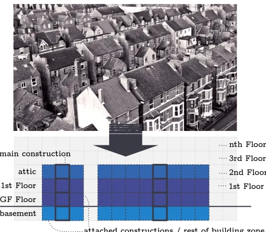
screening methods [48, 49], which compare the uncertainties in the inputs

to those in the outputs. The Morris method (also called the elementary

420

effects method) is the technique most often used in this domain. Here, each

input variable takes a discrete number of values that are chosen within

lim-its defined by their statistical properties. The method provides a measure

of the mean value, µ, which estimates the overall effect of the input on the

output, and a measure of the standard deviation,σ, that estimates

second-425

and higher-order effects of the input variable [50, 48]. This process is

out-lined in Figure 8 where the set of variations is assigned in the input data

set, enabling the possibility to compare against a baseline.

The enriched cuboids, global, and OAT analyses are performed to

iden-tify the most influential parameters in the data set, many of which have been

identified in previous studies [40, 43, 51, 45]; albeit using different simulation

workflows. In EnHub, they are directly included in the simulation platform.

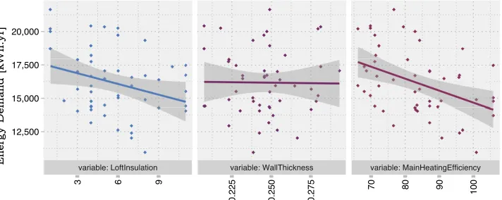
For example, Figure 4 presents results from the application of SAs by

con-trolling changes to the properties of elements contained in the catalogue of

properties used to generate idfs, and by modifying the reduced data set (or

435

indeed by modifying properties related to the external environment, such

as weather files). Figure 4a shows that changes in loft (sometimes known

as attic) insulation and heating system efficiency significantly affect the

en-ergy performance; more so than increasing the wall thickness, as indicated

by their gradients. Figures 4b and 4c compare two output variables by

ap-440

plying a screening method, which makes it possible to combine variables of

different class. Each input variable defines a dimension for the analysis in

which a trajectory of perturbation is defined. The trajectory is chosen by

advancing within the same dimension or to one other. In other words, any

input variable can be selected and changed from an initial stage, but this

445

is limited to the next possible value, either forwards or backwards in its

own dimension. The input change constitutes the next initial stage, and so

the trajectory is developed. This allows comparisons between the discrete

values of each input variable with those of the output. There is widespread

agreement that this method is versatile and useful [48, 49], but the

comput-450

ing time increases significantly and so its application to large data sets is

limited. EnHub accomplishes this analysis by selecting variables based on

expertise, and their use in national programmes and policies.

The results of the SA module are consistent with those presented in

previous studies [43, 51], where a rank of parameters establishes that the

455

differential of temperature between the outside and the inside of a dwelling

systems (space and DHW), and infiltration rates. Thermal transmittance

(commonly known as U-values) is also prominent, especially for walls, as is

the number of occupants, although this value is limited in impact since it is

460

decoupled here from the associated activities (e.g. use of appliances).

Similarly, yet limited in previous studies due to poor representation of

external parameters, solar energy technologies and socio-demographic

vari-ables are identified by the OAT analysis as being significant, and so they

are directly included into the model archetypes. Moreover, the original units

465

of the data set are directly derived from the EHS, which in turn uses the

Postcode Address File (PAF) and the Lower-Super Output Area (SOA) to

define their weights4, which are used to represent the whole English

hous-ing stock. These units are selected randomly and merge information from

nearby PAFs, and the extrapolation is delimited by census subtotals. The

470

inherent bias in this method, because of the generalisation of categorical

variables, affects solar-related parameters, and the definition of

representa-tive households. Thus, improving the quality of information describing these

variables would improve their significance.

[Table 2 about here.]

475

[Figure 5 about here.]

Once the data set has been reduced, the units are re-weighted, and their

tenure and regional information are re-calibrated following a method

em-ployed by many other nationwide surveys [52] (see 6-10 in Algorithm 1).

4_{A weight, or weighting variable, assigns a value to a given case in a data set to}

This method compensates for the assumptions made in the sampling process

480

which, as in the EHS, introduces a loss and bias of information [51]. The

im-pact of this reduction affects the performance of the simulation algorithms,

because their inputs may not exist or may be over-generalised. Hence, there

is virtue in developing a modular approach to construct archetypes,

inde-pendently.

485

[Figure 6 about here.]

2.3. Step 3: Archetype Construction

The set of geometrically simplified models are constructed in a modular

fashion, following an Object-Oriented Modelling (OOM) approach;

essen-tially a collection of interacting objects, where each object is semantically

490

defined with variables, classes and dependencies [53]. An OOM approach

provides the ability to detach specific sections of the modelling process, so

that they can be refined independently. OOM can be represented

graphi-cally using the Unified Modelling Language (UML) architecture to provide

a clear and unambiguous structure for the model attribution workflow, and

495

to enhance the integrity of the predictions of the algorithms used to

de-scribe the energy flow pathways [54]. That is, the architecture shows the

logic in which the components are considered, as well as the distribution

and interrelationship of inputs and outputs used throughout the platform.

EnHub utilises a UML class diagram type (CD), focussed on the

char-500

acteristics of the modules and their relationships. Similar implementations

have been used elsewhere to improve the development of highly detailed

libraries of classes to support more robust management of databases and

modelling algorithms [17, 55]. The EnHub approach is based on both the

idfdocumentation [56, 11] and the BREDEM structure [57], applied using

the CHM protocol [58]. The UML architecture is presented in Figure 6 and

its main components (that form the archetype-specific idfs) are summarised

in Table 3.

To link the EHS with the archetype-specific idf modules, a base case

idfis developed where variable flags5 are used to represent instances of the

510

UML classes. In this way, each EHS sample unit can be associated with its

corresponding property fields and used to structure, scale and attribute the

volumetric archetype appropriately. These archetypes are explicitly

repre-sented as sets of contiguous cuboids (see Figure 7a) that account for the

number of floors and the presence of attics, basements, and attachments

515

such as extensions and conservatories; Table 1 summarises the variables

used to built such a base case. Specifically, an array of cuboids is built by

processing the archetype information; cuboids attached to the main zone,

either on top or at the sides, can then be scaled or removed as required.

This helps to maintain the connection of shared surfaces. In this way, it is

520

possible to represent the key residential types of the stock, such as detached

houses, semi-detached, end of terrace, mid terraced, flats (also known as

apartments) and bungalows (see Figure 7b). These forms, complemented

with their semantic attributes, comprehensively and robustly describe the

derived stock of archetypes, but are now based on an explicit volumetric

525

representation (see Figure 7c).

[Figure 7 about here.]

The volumetric representation used by an idf includes the assignment

of internal zones. EnHub follows the BREDEM representation, using two

5

zones. These are initially defined in each cuboid archetype using a main

530

zone, and a distinct secondary zone that represents the rest of the building.

For example, in Figure 7a, the ground floor (GF) is initially assigned to the

former, whereas the basement, the first floor (1F) and a room in the roof (in

some cases, interchangeably referred to as attic), are assigned to the latter.

The attached constructions are employed to incorporate differences between

535

detached dwellings and those forming terraced rows. Moreover,

relation-ships between openings (i.e. windows, doors, accesses) and total floor areas

are defined for each zone. In Figure 7b, the semi-detached house, as shown

in the middle, increases the number of surfaces at whichEnergyPlus

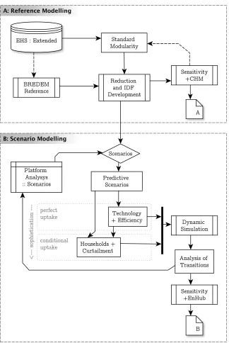
simu-lates solar radiation. Hence, the relevance of a volumetric representation of

540

archetypes, and the need to appropriately characterise openings.

Employing a base caseidfto construct the volumetric archetypes helps

to respect EnergyPlus’s precise coordinate structure. Furthermore, whilst

idfproperty fields can be combined in any order, it is convenient to follow

the sequential structure of the EnergyPlus format [56, 11], because this

545

helps with the readability in the representation of our archetypes, and the

convenience with which their attributes may later be manipulated. The

steps involved in adapting the base case idf are described in the pseudo

code shown in Algorithm 2.

Algorithm 2Construction, simulation and analysis of archetypes;

Notation: h,imeansis a subset of

550

1. c o n s t r u c t d w e l l i n g a r c h e t y p e s for s i m u l a t i o n ;

s r e p r e s e n t s the s i z e of the d a t a set e m p l o y e d

l o o p :

for i:=1 to s do

sA−general←f(SAP,hEHSi) 555

sB−location←f(SAP, ON S,hEHSi)

sC−schedules←f(ON S,hEHSi)

sD−envelope←f(ON S,hEHSi)

sE−geometry←f(ON S,hEHSi)

sF−internal←f(SAP, ON S,hEHSi) 560

sH−water←f(SAP, ON S,hEHSi)

sI−outputs←f(EP lib,hEHSi)

d o n e

565

2. s i m u l a t e d w e l l i n g a r c h e t y p e s l o o p :

for i:=1 to s do

simulation←f(i, weatheri, schedulesi)

d o n e

570

3. a n a l y s e s i m u l a t e d d w e l l i n g a r c h e t y p e s l o o p :

for i:=1 to s do

summary←f(i, EHS, Outi)

575

derived←f(i, EHS, Outi)

A catalogue of appliances and heating systems is included in the base

case idf to describe internal gains. Their specifications (i.e. power,

effi-ciency and heat gains) and fuel sources are defined using the EHS and the

580

Energy Consumption in the UKtables [59]. Similarly, household water

ser-vices are included in theidfs, although they are reduced to a total annual

demand. Occupants and their associated (estimated) metabolic gains are

also included, and can be directly linked to specific intensity values, such as

heat gain per person and floor area per capita.

585

The dynamic actions of devices and occupants are emulated using

sched-ules. These include time-related events, such as occupant presence, or the

use of appliances, window openings, heating systems, and water fixtures.

The schedule profiles are prepared for each model by applying a

probabilis-tic function that is dependent on the properties of each archetype, such as

590

the household composition or dwelling type (see the pseudo code shown in

Algorithm 3). This means that even though profiles follow similar patterns,

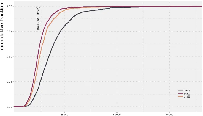
each element is unique. This approach enables the behaviours of a specific

group of archetypes to be analysed. The resolution of a schedule is

indepen-dent of the model, but they are conveniently paired with the computational

595

for each day type are built for an entire year, but they can be seasonal.

Algorithm 3Probabilistic profile generation

1. e x t r a c t p r o f i l e f r o m n a t i o n a l a v e r a g e d a i l y p r o f i l e s

Mn ← e x t r a c t ( d a t a : a v e r a g e u s a g e ); n e l e m e n t s

600

2. e x t r a c t r e p r e s e n t a t i v e h o u s e h o l d p a r a m e t e r s

Hhp ← e x t r a c t ( d a t a : h o u s e h o l d ); p p o p u l a t i o n

3. a s s i g n a p r o b a b i l i s t i c f u n c t i o n to e a c h p r o f i l e

605

b a s e d on a v e r a g e d a i l y u s a g e

dn ← P(Mn)

4. c r e a t e r a n d o m p r o f i l e b a s e d on p -f u n c t i o n for

a g i v e n p e r i o d

610

l o o p :

for i:=1 to 1 0 1 6 do

for j:=1 to n do

for k:=1 to 365 do

r a n d o m i s e (Hhi, djk)

615

In the same vein, EnHub uses a library of standardEnergyPlusWeather

(EPW) files to describe local environmental conditions for the defined

pe-riod. The appropriate weather files, used by EnergyPlus, are associated

according to the regions that the model archetype has explicitly been

allo-620

cated to. The regions are aligned to the resolution provided by the EHS:

NUTS-16 level, which encloses subdivisions of the four UK countries, and

is regulated by the European Union. These EPW files are synthesised Test

Reference Years (TRYs), where each month represents an average over a

period of around 20 years. Each month may come from a different year,

625

and so they are combined using a cubic spline method [60]. This method

interpolates the data when gaps and inconsistencies are present.

[Table 3 about here.]

6

2.4. Step 4: Dynamic Simulation

As noted earlier, the platform architecture has been designed to provide

630

for both flexibility and scalability. For example, it can simulate a single

archetype and systematically modify the parameters of A1 and C2 (see

Table 3) to increase temporal resolution; it can employ a OAT sensitivity

analysis module to analyse key independent variables (fabric properties, use

intensity, devices efficiency) for one or more archetypes; or it can simulate

635

the entire UK housing stock to evaluate different scenarios (see Sections 1

and 3). Analyses can also be geographically constrained, to simulate the

housing stock of a city. This scalability results from the ability to detach

processes, as well as from the aforementioned modularity.

The whole stock is simulated for an entire calendar year, plus an

addi-640

tional preheating period, at an hourly resolution. This resolution is

reason-able, given that we are not explicitly modelling ventilation, nor accounting

for the associated stochastic behaviours of occupants (although this will be

amended in the future); we simply utilise a fixed infiltration rate, and

ven-tilation heat gain schedules. Each simulation takes around 30 seconds to

645

complete using a single core high-end computer7_{. However, multiple}

simula-tions of the 1016 archetypes are required and so the workflow is coupled with

a High Performance Computing (HPC) cluster8_{, to reduce the simulation}

time by over 98%. Figure 1 presents the conceptual structure of EnHub and

shows the communication paths between the components of the platform

650

and the tools required to support it.

7

Software specifications: EnergyPlus version 8.4, R version 3.2; Hardware specifica-tions: Processor Intel Core i5 2.9 GHz CPU, 16 Gb RAM

8_{166 compute nodes (Dell C6220), with 2x 8-core processors (Intel Sandybridge}

2.5. Step 5: Iterative Analysis

The derived energy performance indicators are processed in R so that

they can be conveniently stored and compared. Thermal comfort indicators

are computed in EnergyPlusbased on the ASHRAE-55 standard [56], but

655

in the future they could be readily complemented with other indicators of

instantaneous comfort, or of over- or under-heating risk, by post-processing

theEnergyPlusresults within EnHub.

Each batch of simulations of the 1016 archetypes is stored in a database,

in which multiple (input, output and auxiliary) data sets are linked by

com-660

mon identifiers (see Figure 8); enriching analysis options. SA is employed

both for reference modelling (choice of archetypes and parameters to

sam-ple from) and scenario modelling (choice of parameters to act on). Figure 8

shows that there are two stages to the simulation process: the first stage

(A) focuses on data resolution, whereas the second (B) focuses on modelling

665

parsimony and the study of different scenarios.

[Figure 8 about here.]

3. Application to Evaluate De-carbonisation Scenarios

Here we deploy the EnHub platform to evaluate a baseline and a series

of measures that are designed to reduce UK housing stock carbon intensity.

670

3.1. Definition of Scenarios

The workflow summarised in Figure 1 is used to test twoCO2 reduction

scenarios that are adapted from national policies [61, 62, 4, 63]. The first

emulates a perfect uptake scenario, where the fabric properties and

appli-ances of dwellings are upgraded to be as efficient as is plausibly possible,

regardless of their current values, associated costs, or the level of

disrup-tion in adopting them. The second is a conditional uptake scenario (see

the pseudo code shown in Algorithm 4), where the upgrade is limited to a

fraction of the stock represented by a particular archetype, and considers

real-life constraints, such as costs, disruption, and the initial values of the

680

parameters of interest; so diminishing the likelihood of uptake of measures

that entail marginal gains or heavy disruption.

Algorithm 4Implementation of conditioned uptake scenarios

1. o b t a i n t e c h n i c a l p o t e n t i a l of i m p l e m e n t a t i o n

technicali←f(savings, trigger, uncertainty)

685

2. o b t a i n i n c o m e / f u e l e x p e n d i t u r e r a t i o

incomei←f(income, trigger, uncertainty)

3. o b t a i n t y p o l o g y f e a s i b i l i t y p a r a m e t e r

690

contraintsi←f(current, trigger, uncertainty)

4. o b t a i n r e t u r n of i n v e s t m e n t r a t i o

roii←f(cost, trigger, uncertainty)

695

5. i n c l u d e r a n d o m u p t a k e p r o c e s s

randomi←f(individual, trigger, uncertainty)

6. e v a l u a t e w i t h t h i e r c o r r e s p o n d i n g u p t a k e t r i g g e r s i: h o u s e h o l d s

700

Ui←f(technicali, incomei, contraintsi, roii, randomi)

[Table 4 about here.]

The selected scenarios and associated measures are summarised in

Ta-ble 4, which describes the current status of the dwellings, and the variations

705

that are then parsed to the model, with each scenario considered in isolation.

For each scenario, an additional case is tested to understand the

implica-tions of different occupancy profiles and patterns of usage; these are based

on average profiles defined in the Energy Consumption in the UK study

[4]. Here, multiple profiles are defined based on their existing probabilistic

distributions [4], so that the values relate to each archetype, and to each

element associated with an activity (as previously shown in Figure 3).

3.2. Results

[Table 5 about here.]

[Figure 9 about here.]

715

Table 5 and Figure 9 summarise the outcomes from the perfect and

conditional uptake scenarios, whose measures are given in Table 4. They

show that when perfect uptake is assumed, A02 and A01 have the greatest

impacts, arising from improved fabric performance. Other impactful

scenar-ios are A05, A08, and A06; these latter two being partially counteracted by

720

increased heating loads, affecting indoor temperature. When household

con-straints are considered in respect of scenario 02 (A01 to B02), the potential

emissions reduction is reduced by around 40%. The constraints considered

in measures B01-B07 are related to the disposable income of a household

or to the increased costs associated with more technically challenging cases,

725

such as housing in conservation areas, solid masonry walls in old buildings,

or the insulation of loft spaces that are used for storage purposes with limited

accessibility.

[Figure 10 about here.]

The combined scenario (A01+A02) has a relatively high impact on

en-730

ergy demand reduction (319 TWh, 25% less than the baseline). Table 5

shows that their combination is roughly equivalent to all the scenarios

com-bined (All). Likewise, Table 5 outlines the associated potential to reduce

some of the benefits of the individual measures overlap, so that the outcome

735

is not the simple arithmetic sum of each respective saving, and so combining

multiple measures does not guarantee a substantial improvement. This can

be seen, for example, in Figures 9 and 10 that reveal the extent to which

energy demand is reduced by combining all the measures.

[Figure 11 about here.]

740

Improvements to the fabric may be more likely to be viable for old and

large dwellings because of the relatively poor performance of their fabric

elements, and their relatively large surface areas. However, sometimes the

spaces within these type of buildings have been repurposed and cannot be

modified. For example, it is difficult to install energy conservation measures

745

in a loft that has been designated for storage. Figure 11 outlines the

pro-portion of dwelling typologies (by epoch and type) in terms of accumulated

floor area in the housing stock. This helps to identify the archetypes that

have particular decarbonisation potential, or lack of. For example, pre-1919

terraced dwellings accumulate the greatest floor area in the stock, but their

750

uptake potential is limited by the aforementioned constraints.

[Figure 12 about here.]

Figures 12a and 12b outline differences in the energy intensity of dwellings

by archetype. The area formed by the axis variables represents the total

energy demand (428 TWh for the baseline case). This helps to better

un-755

derstand the effectiveness of the different measures, particularly when there

are real-world constraints that affect their implementation. For instance,

Figure 12a shows that, even though the accumulated energy demand

be seriously constrained. Figure 12b shows that apartments are particularly

760

sensitive to our modelled perfect uptake measures; albeit constrained by the

relatively small cumulative floor area.

[Figure 13 about here.]

Figure 13 suggests that renovation measures may impact on occupants’

thermal satisfaction, as the mean indoor temperature is elevated (relative

765

to the base conditions) by around +0.8 K. This is due to indoor air

temper-atures that exceed the heating system set-point when it is on (due to excess

solar gains), or are higher when the heating system is off (due to better

con-servation of energy). These improvements are expectedly more noticeable

in the cold season, reducing energy bills among the population. Due to a

770

lack of supporting data, any co-benefits to carbon emissions and comfort

levels that arise from renovation measures are ignored here (meaning that

potential energy savings may not be fully realised due to improved comfort

from higher indoor temperatures).

Finally, while scenarios A06-07 and B06-07 show that substitutions of

775

lights and appliances are low-cost upgrades with a quick return on

invest-ment, they are not very effective. Increasing the efficiency of appliances is

clearly a quick and easy way to reduce electrical energy demand, but this

can be counteracted by increased heating demands.

The study of scenarios is useful because it enables the quick and

conve-780

nient exploration of the limits of potential impacts arising from related

poli-cies or strategies. The testing of scenarios that consider the conditional

up-take of measures gives an understanding of potential to upup-take constraints;

but they do not shed light on probable outcomes. This would require a

thorough understanding of the underlying drivers affecting the uptake of

energy-related improvements by households, and the associated trade-offs

between energy demand, costs, comfort, and convenience; likewise, changes

to energy-using practices. EnHub will be continually improved to facilitate

more granular analyses, and to integrate a platform simulating occupants’

energy-using behaviours and associated adaptive comfort, as well as a

so-790

cial simulation platform to predict changes in households’ investment and

energy-using behaviours.

This combined platform has the potential to considerably improve upon

the ability to reliably diagnose where the greatest potential for socio-technical

innovation lies on the one hand—with a view to decarbonise the housing

795

stock; and to design, test and implement policies and strategies to realise

this potential on the other.

4. Conclusion

This paper presents a new open-access modular platform for the dynamic

simulation of the UK housing stock—EnHub, with a view to efficiently

eval-800

uating the effectiveness of national decarbonisation strategies. At present,

this is restricted to the analysis of the possible implications from perfect

or assumed uptake of these strategies, whether physical (building envelope,

systems and appliances), or behavioural.

Housing stock decarbonisation is a long-term endeavour that requires

805

constant updates to the evidence base and recalibration of models. We

believe that EnHub can facilitate better inter- and trans-disciplinary

col-laboration, by providing a standardised hub to combine data models from

different perspectives. We also believe that an open-source dynamic

simula-tion platform, such as EnHub, offers greater utility and longevity, compared

to its closed and steady-state counterparts. This is reinforced by making

each component, of the semantically attributed 3D representations of the

archetypes comprising the UK housing stock, editable and verifiable.

To facilitate widespread accessibility, EnHub may be downloaded, upon

signing a by-attribution license agreement, from the open source version

815

control repository GitHub. This also helps to facilitate and manage

con-tributions from other potential developers of EnHub—further enriching its

future functionality. Furthermore, work is currently underway to improve

the usability of EnHub, through a graphical user interface. In principle, this

may widen the user base from those interested in national decarbonisation

820

policy, to include those that are interested in regional and city scale

de-carbonisation policy and planning interventions—by including geographical

constraints in its application.

Finally, to address the above restriction of assumed uptake of

decarbon-isation strategies, we plan to facilitate the combined modelling of household

825

investment behaviours, and their responses to changes to the underlying

drivers that influence them (e.g. regulatory, financial, educational, social,

technical), and energy-using behavioural practices; this latter through

in-tegration with the multi-agent stochastic simulation platform Nottingham

Multi-Agent Stochastic Simulation (No-MASS) [64].

HPC

data

shell

Figure 1: Steps involved in the application of EnHub. The statistical platformRis em-ployed to perform all the steps. The computationally-intensive tasks, such as the simula-tion step, can be performed using a different hardware whereEnergyPlusis installed.

835

●

r = 0

r = 0.2

r = 0.4

r = 0.6

r = 0.8

● ● ● ● ● ● ● ● ● ●_● ●● ● ● ● ● ● ● ●● ●● ● ● ● ● ● ● ● ●● ● ● ● ● ●● ●● ● ● ● ● ● EPGskWh arnatx fmodule felorin northxs region ageband type isattic iscellr floors AttchSt heatrrd agbndrd Inccat flatare typrstr felxtff cvtylft wllcnst wllThck elecmop fpindf unoc ageprtx fnchtyp watrsys hsstryx cellarh storysw storysd storysh cllrwxt cllrhxt stryshx fcdhght manfxtr ● aglflrr_●lsf fltblckisbnglw fltflrs flath flatarx fpfllnc spahcst cookcst TFA . . ●_mainfa

(a) Gas Demand

●

r = 0

r = 0.2

r = 0.4

r = 0.6

r = 0.8

● ● ● ● ● ● ● ● ●● ● ● ● ● ● ● ●● ● ● ● ● ●●● ● ● ● ● ● ● ● ● ● ● ● ● ● ● ● ● ● ●●● ● ● ● CO2eqkg arnatx fmodule felorin northxs region ageband type isattic iscellr floors AttchSt heatr agbndrd Inccat flatare typrstr felxtff cvtylft wllcnst wllThck elecmop fpindf unoc ageprtx fnchtyp watrsys hsstryx isbnglw _cellarh storysw rdstorysd storysh cllrwxt cllrhxt stryshx fcdhght mainfa manfxtr aglflrr _lsf

fltbfltflrslck

flath flatarx fpfllnc spahcst cookcst TFA . .

(b) Carbon Emissions

●

r = 0

r = 0.2

r = 0.4

r = 0.6

r = 0.8

● ● ● ● ● ● ● ● ● ● ●● ● ● ● ● ● ● ●● ●● ● ● ● ● ● ● ●● ● ● ● ● ● ● ● ● ● ● ●● ● ● ● ●● IntrnlT arnatx fmodule felorin northxs region ageband type isattic iscellr floors AttchSt ●heatrrd agbndrd Inccat flatare typrstr felxtff cvtylft wllcnst wllThck elecmop fpindf unoc ageprtx fnchtyp watrsys hsstryx isbnglw _cellarh storysw storysd storysh cllrwxt cllrhxt stryshx

fcdhghtmainfa manfxtr

aglflrr lsf fltblckfltflrs flath flatarx fpfllnc spahcst cookcst TFA . .

(c) Internal Average Temperature

Figure 2: Focused Principal Component Analysis (FPCA) visualisation. The estimated energy demand in the models is the sum of fuel energy demands, in which (a) considers the main fuel used in the stock. To identify other variables affecting the overall energy demand, (b) considers the associated carbon emissions, which is directly dependent of

100 200 400 800 3200 1600 6400

0 250 500 750 1000 1250

iterations: sample size

100 200 400 800 1600 3200 6400 160.0% 120.0% 80.0% 40.0% ob jectiv e criterion

(a) 3 pivotal variables - from Table 1

100 200 400 800 3200 1600 6400 99.8%

100.0% 100.2% 100.4%

0 250 500 750 1000 1250

iterations: sample size

100 200 400 800 1600 3200 6400 ob jectiv e criterion

(b) 7 pivotal variables - from Table 1

100 200 400 800 3200 1600 6400

0 250 500 750 1000 1250

iterations: sample size

100 200 400 800 1600 3200 6400 180.0% 150.0% 120.0% 90.0% ob jectiv e criterion

(c) 40 pivotal variables - from EHS

Energy

Demand

[k

Wh.yr]

(a) Global SA - insulation, thickness, efficiency. The Confidence Interval (CI) is determined by applyinglocally weighted scatterplot smoothing.

250 500 750 1000 1250 1500 1750 2000

750 1500 2250 3000 3750 4500 5250 6000 ∆ differential mean [kWh]

standard deviati on [k Wh] BASE AOc FHg HEf FCn Dft WTk WAr LIn Reg WTy

(b) Screening Method - energy demand reference 0.200 0.400 0.600 0.800 1.000 1.200 1.400

0.100 0.200 0.300 0.400 0.500 0.600 0.700 0.800

∆ differential mean [K]

standard deviati on [K] BASE AOc FHg HEf FCn Dft WTk WAr LIn Reg WTy

(c) Screening Method - indoor tempera-ture reference

Figure 4: Examples of the SA module: screening method

0 100 200 300 400 2 3 4 5 6

0 100 200 300 400

2 3 4 5 6 2 0 4 0 6 0 8 0 1 0 0 2 .0 2 .2 2 .4 2 .6 2 .8 GFArea G F S to re y H e ig h t GFArea G F S to re y H e ig h t LHS dataset survey dataset G F S to re y H e ig h t G F A re a

sample | survey

(a) GF dimensions

L SE EoE SW WM EM NW YaTH NE

la oo pr R

Tenure Tenure

Regi

on

la oo pr R

Survey LHS

(b) Region and tenure variables