Cloud based e Infrastructure for scheduling astronomical observations

Cloud-based e-Infrastructure for Scheduling

Astronomical Observations

James Wetter

, ¨

Ozg¨ur Akgun

, Adam Barker

, Martin Dominik

, Ian Miguel

, Blesson Varghese

∗_{School of Computer Science}

University of St Andrews

Email:{jpw3, ozgur.akgun, adam.barker, ijm, varghese}@st-andrews.ac.uk

†_{School of Physics & Astronomy}

University of St Andrews Email: [email protected]

Abstract—Gravitational microlensing exploits a transient phe-nomenon where an observed star is brightened due to deflection of its light by the gravity of an intervening foreground star. It is conjectured that this technique can be used to measure the abundance of planets throughout the Milky Way. In order to undertake efficient gravitational microlensing an observation schedule must be constructed such that various targets are observed while undergoing a microlensing event. In this paper, we propose a cloud-based e-Infrastructure that currently supports four methods to compute candidate schedules via the application of local search and probabilistic meta-heuristics. We then validate the feasibility of the e-Infrastructure by evaluating the methods on historic data. The experiments demonstrate that the use of on-demand cloud resources for the e-Infrastructure can allow better schedules to be found more rapidly.

I. INTRODUCTION

Gravitational microlensing is a transient phenomenon where the light received from an observed star is bent by the gravita-tion of an intervening foreground star leading to an observable characteristic brightening, lasting about a month [1], [2]. A planet orbiting the foreground star can reveal its presence by creating a further small dip or blip on the otherwise symmetric light curve [3], [4].

Given that the probability for a given star to be significantly brightened at any given time is quite small (about one in a million) [5], a three-step strategy of survey, regular follow-up, and anomaly monitoring arose [6], [7], [8]. In order to find a substantial number of gravitational microlensing events, hundreds of millions of stars are monitored at least daily by dedicated surveys and if microlensing events are detected or suspected at a given target monitoring frequency is increased to enable proper characterisation. Both the Optical Gravitational Lensing Experiment (OGLE) and Microlensing Observations in Astrophysics (MOA) surveys, together detect-ing more than 2000 microlensdetect-ing events per year, operate real-time data reduction systems that report photometric data of ongoing events promptly to the scientific community [9], [10]. With the resources for follow-up observations being limited and detected microlensing events being in oversupply, a well-informed decision needs to be made about how to distribute

the available observing time amongst the potential targets so that the scientific return is being maximised.

The rapid construction of an observation schedule is highly desirable because event observation priorities change substan-tially on time-scales as short as a few minutes and the avail-ability of telescope resources for observations also come with little predictability, given that we are dependent on the weather. We note that robotic telescopes have the technical advantage of flexible scheduling and prompt reaction. However, the design of software to efficiently schedule observing campaigns across several telescope networks explicitly needs to support both the science requirements of the campaign and the capabilities of the telescopes. A variety of scheduling problems arising in astronomy have been studied previously [11], here we present a novel approach designed specifically for microlensing ob-servation schedules.

Because unpredictable weather conditions can interrupt ongoing observations, rapid rescheduling at short notice is a priority. As scheduling over even a 24 hour horizon is computationally intensive large computational resources need to be available on-demand.

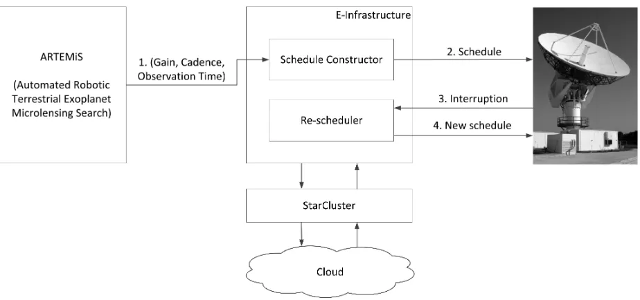
Fig. 1. Architecture of e-Infrastructure for scheduling astronomical observations.

e-Infrastructure.

The e-Infrastructure we have developed currently constructs observation schedules for a single telescope. The quality of the generated schedules is determined by a metric we have proposed that rewards high value targets being regularly observed with ideal regularity. This metric also accounts for interrupted observations and subsequent rescheduling. The e-Infrastructure supports four techniques to construct high quality observation schedules, including a greedy algorithm, two different hill climbing searches and a simulated annealing search. The e-Infrastructure supports parallelisation via the deployment of a portfolio of these techniques on a large pool of cloud based resources. A key observation is that the e-Infrastructure allows the performance of the scheduling system to scale with the amount of computational resources used, thus allowing a user to easily adjust the investment in computational infrastructure with the quality of schedule required.

The remainder of this paper is structured as follows. Section II presents the architecture of the e-Infrastructure. Section III provides the solution techniques employed in the e-Infrastructure to generate schedules. Section IV considers the problem of rescheduling when there is an interruption. Section V confirms the feasibility of the infrastructure and presents the empirical evaluation of the techniques on historic data. Section VI concludes this paper by presenting future work.

II. E-INFRASTRUCTUREARCHITECTURE

The e-Infrastructure we have designed obtains input from the ARTEMiS (Automated Robotic Terrestrial Exoplanet Mi-crolensing Search) system [14] and is intended to interact with a telescope as shown in Figure 1. There are two main compo-nents, namely (i) the Schedule Constructor, which generates a

schedule for the telescope based on the input data (considered in Section III), and (ii) the Re-scheduler, which reschedules the telescope when there is an interruption due to unpredictable weather (presented in Section IV). Both components harness the computational resources on the cloud for generating the schedules. In this research, the e-Infrastructure makes use of the Amazon Web Services (AWS)1 _{Elastic Compute Cloud}

(EC2)2 _{virtual machines. The e-Infrastructure facilitates the}

management of the components on AWS and is supported by the MIT StarCluster3 for managing the AWS resources. StarCluster facilitates the automatic configuration and launch of AWS EC2 VMs as a cluster and in addition allows for adding or removing VMs from a cluster which is leveraged in the e-Infrastructure.

A. Input

With the aim to infer planet population statistics from microlensing observations, the detection efficiency of our campaign should be as large as possible. We adopt a priority-cadence-exposure time paradigm, in which these three param-eters per target completely characterise the campaign strategy. These parameters are:

i. a gain factor that accounts for the importance of the tar-get and the resources consumed by the observation [15], ii. a cadence interval that represents the ideal time interval

between observations, and

iii. an exposure time that represents the length of an obser-vation.

The gain factor allows the prioritisation of events and can be straightforwardly evaluated from the current properties of the event [16], as carried out in real time by the ARTEMiS

system. The values of the cadence interval and exposure time have not been systematically studied, but practical experience from the PLANET (Probing Lensing Anomalies NETwork) campaign [7] has resulted in methods to calculate these values.

B. Quality of Schedules

In order to construct high quality schedules we must for-mally specify a quality metric. In this section we present such a metric.

Given a set of targets, S, that can be observed each target, s ∈ S, has a gain (Ωs), a cadence (τs) and an observation

period (ts) calculated as described above. We need to plan

an observation schedule for a single telescope, ˆv ∈ Sn, of a fixed length n. We use vi to refer to the ith target of the

schedule v. The targets are always scheduled to be observedˆ for the exact duration of their exposure time. A good schedule will contain repeated observation of targets with high gain, spaced according to their cadence. Our quality metric linearly decreases the gain of a target as repeated observations deviate from the ideal cadence. Formally we have;

qual (ˆv) = n

X

i=1

r(ˆv, i, vi), (1)

where

r(ˆv, i, s) = Ωs·(τs− |e(ˆv, i, s)−τs|)/τs, (2)

ande(ˆv, i, s)is the time between the most recent observation ofsand sloti, with a default value ofτsifshas not yet been

observed.

The quality metric is then used by the e-Infrastructure to construct a high quality schedule by the Schedule Constructor considered in the next section.

III. SCHEDULECONSTRUCTOR

The e-Infrastructure needs to construct an optimal schedule as determined by the metric defined above. The construction of valid or optimal combinatorial structures, such as this schedule, is a common problem tackled in artificial intelli-gence [17]. While it is not hard to find a valid schedule (any sequence of targets is valid), it remains hard to find an optimal schedule because the number of possibilities is enormous. For example, one historic instance of this scheduling problem requires scheduling observations for 1763 targets over a 24-hour period allows 1763720_≈2×102337 _{possible schedules.} Clearly, this space can not be enumerated in practice. For this reason the e-Infrastructure employs incomplete probabilistic methods to construct good, but sub-optimal, solutions within a reasonable time.

A. The GREEDY Algorithm

A simple technique often used to solve combinatorial prob-lems is a greedy heuristic. Such a technique makes choices that are locally optimal. This rarely results in the best possible solution, but often provides a good compromise between time complexity and solution quality [18].

Here the greedy approach constructs a schedule chrono-logically by choosing the most promising target for each observation slot, in the context of the observations already planned. Pseudocode for this procedure is shown in Figure 2.

1: procedure GREEDY(v,ˆ S, i)

2: forj←i, ndo

3: vj ←arg maxs∈Sr(ˆv, j, s)

4: end for

5: returnvˆ

6: end procedure

Fig. 2. Complete the suffix of schedulevˆfrom indexitonwith targetsS using a greedy approach.

B. Local Search

Another common approach to solving combinatorial prob-lems is to search the space of possible solutions, the so-lution space, until a suitable solution has been found. For problems with a solution space too large to be exhaustively enumerated incomplete approaches, such as local search, are often employed. Local search algorithms function by applying local changes to an incumbent solution to move through the search space until a computation limit is reached, or a suitable solution is found [18]. To perform a local search two mechanisms are required;

i. the construction of an initial candidate solution and ii. the construction of a neighbour of a given solution. An initial solution can be constructed via the GREEDY

algorithm. The neighbourhood of a schedule can be defined by replacing any planned observation with any other target, and then using GREEDY to adjust the suffix of the schedule. Pseudocode for constructing a single neighbour is shown in Figure 3. We refer to this neighbourhood as NH1.

1: procedure NEIGHBOUR(ˆv,S)

2: i←UNIFORM(1, n)

3: vi←GETTARGET(ˆv, i,S\ {vi})

4: ˆv←GREEDY(ˆv,S, i+ 1)

5: returnvˆ

6: end procedure

7: procedure GETTARGET(v, i,ˆ S)

8: S0←TAKE(|S|/100,SORTBY(λs.r(ˆv, i, s),S)) 9: returnUNIFORM S0

10: end procedure

Fig. 3. Compute a neighbour of schedulevˆusing observation targets S. UNIFORM(i, j)chooses a random integer betweeniandjinclusive, according to a uniform distribution. GETTARGETreturns a random element from the top 1% ofSas evaluated byr(ˆv, i, s).

This neighbourhood is heavily biased toward alterations to the tail end of a schedule, a change to the final target,vn, of the

we alternate the direction of the greedy construction each iteration of the algorithm, every second iteration we reschedule forward from the altered target to the end of the schedule and every other iteration we schedule backward from the altered target to the first unscheduled observation. We refer to this neighbourhood as NH2. The two methods of constructing neighbours are empirically evaluated in Section V-A.

A simple local search technique that makes use of such neighbourhoods is hill climbing, also known as gradient descent. This method generates a neighbour of the incum-bent solution and if this neighbour is an improvement the incumbent solution is updated and the search continues [18]. Pseudocode is presented in Figure 4. The parameter NHOOD is a function that generates a neighbour for the given schedule, it can be either NH1 or NH2.

1: procedureHILLCLIMBING(v,ˆ S,NHOOD)

2: vˆ0←NHOOD(ˆv,S) 3: if eval(ˆv0)>eval(ˆv)then

4: OUTPUT(ˆv0)

5: HILLCLIMBING(ˆv0,S,NHOOD)

6: else

7: HILLCLIMBING(ˆv,S,NHOOD)

8: end if

9: end procedure

Fig. 4. Perform a hill climbing search to find high quality schedules. The search continues indefinitely but is terminated externally when a computa-tional limit has been reached.

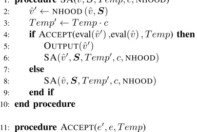
Hill climbing is known to get trapped in local optima restricting the quality of solutions it may discover. Many meta-heuristics have been proposed to overcome this short coming of local search algorithms. A well known metaheuristic, sim-ulated annealing, is applied here. This algorithm, inspired by thermodynamical properties of cooling metal, modifies the simple hill climbing algorithm to allow it to sometimes accept worse solutions during search. The probability of accepting a worse solution is decreased as search progresses [19], [20]. Pseudocode is given in Figure 5.

The different search techniques are empirically evaluated in Section V-A.

IV. RE-SCHEDULER

The e-Infrastructure must be able to deal with unpredicted interruptions to an ongoing observation schedule. For this, two simple methods could be employed without alteration to the quality metric:

i. offset the planned observations and ignore the interrup-tion, or

ii. cancel observations that were scheduled to occur during the interruption.

Neither of these alternatives is acceptable. Simply offsetting the scheduled observations will disrupt the intervals between all remaining observations, vastly degrading the quality of the observations. Cancelling observations could also be costly, as an observation of a target with very high gain may be cancelled

1: procedure SA(v,ˆ S, T emp, c,NHOOD)

2: ˆv0←NHOOD(ˆv,S)

3: T emp0 ←T emp·c

4: if ACCEPT(eval(ˆv0),eval(ˆv), T emp) then

5: OUTPUT(ˆv0)

6: SA(ˆv0_{,S, T emp}0_{, c,NHOOD)}

7: else

8: SA(ˆv,S, T emp0, c,NHOOD) 9: end if

10: end procedure

11: procedure ACCEPT(e0, e, T emp)

12: ife0> ethen

13: returnTrue

14: else

15: r←UNIFORM(0,1)

16: p←exp((e0−e)/T emp)

17: returnp > r

18: end if

19: end procedure

Fig. 5. Perform a simulated annealing search to find high quality schedules. UNIFORM(i, j) selects a random floating point number between i and j inclusive, according to a uniform distribution.

Time

s1 s2 s3 s1 s1

(a) If we ignore earlier observations after a short interruption we may schedule a target twice in rapid succession, as demonstrated by target s1 here. This is not ideal as we have deviated far from the ideal time

interval between observations unnecessarily.

Time

s1 s3 s1

s2 s4 s2

(b) If we retain earlier observations after a long interruption a high value target may never be scheduled again, as demonstrated by targets2here.

This is not ideal because very high value targets can be excluded from further observation.

Fig. 6. Problem cases when recovering from interrupted observations.

where as a slight deviation from its ideal cadence would be a better option. Therefore the quality metric of a schedule has been adjusted to adequately deal with such interruptions.

Consider these two simple ways to respond to interrupted schedules:

i. throw away the observations that have been made so far and plan a new schedule from scratch after the interruption, or

ii. or continue scheduling treating the gap as an observation of a target with zero gain.

choose to observe the same target twice in rapid succession with no penalty, which is not ideal. Now consider a longer interruption such as in Figure 6b. If we continue scheduling treating the interruption as an observation of a zero gain target, then the targets observed previously may be so heavily penalised by the long break in observation that they are never again scheduled. Again, this is not ideal.

A middle ground is to modify the quality metric so it selectively forgets observations before an interruption under certain conditions. Assume an interruption has occurred from timeatoa0_{. We are now scheduling an observation to be taken} timeb > a0_{. When evaluating a particular targets:}

i. if b−a < 2·τs then include previous observation for

gain calculation ofs,

ii. ifb−a≥2·τs then schedulesas if for the first time.

Because these rescheduling events are often triggered by unpredictable interruptions the demand for computational re-sources will be highly bursty. The cloud computing paradigm allows access to a set of resources from a data centre that meets these sudden demands for compute power during rescheduling events and then can be terminated until a further interruption. In this manner, not only is the cloud economical in dealing with interruptions, but also meets the computational require-ments. For this reason the e-Infrastructure relies on cloud based deployment for scheduling.

V. EXPERIMENTS

In this section, the search methods employed in the e-Infrastructure are compared, followed by the parameters em-ployed for the best search method, and finally the deploy-ment of the best search method on the cloud using the e-Infrastructure.

A. Search methods

In order to compare the different search techniques dis-cussed in Section III schedules were constructed for three different instances of historic data from the ARTEMiS system [14]. On each of these instances three different algorithm configurations were run. The configurations used were:

• HC1; hill climbing with neighbourhood NH1,

• HC2; hill climbing with neighbourhood NH2,

• SA; simulated annealing with neighbourhood NH2.

The parameters of the simulated annealing algorithm were tuned for each instance as discussed in V-B resulting in the settings:

• 2013-01-01; initial temperature 1500, cooling rate 0.001,

• 2013-06-01; initial temperature 3000, cooling rate 0.001,

• 2014-01-01; initial temperature 3000, cooling rate 0.001.

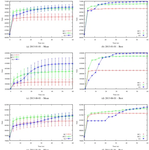
Each combination of instance data and algorithm configu-ration was run with one hundred different seeds. Figures 7a, 7c and 7e show the mean and standard deviation for the runs, and Figures 7b, 7d and 7f show the best solution found by each configuration for each instance.

It is clear that the neighbourhood NH2 is better than NH1 on all instances, for both mean and best results. Also, given the

correct parameters the simulated annealing outperforms hill climbing within an hour across all instances. Finally, it is also worth noting that standard deviation of all methods is quite large, indicating that a single run of any of the algorithms will not guarantee good results. Instead several runs on the same instance data with different seeds is required.

B. Parameters for simulated annealing

As mentioned in section V-A simulated annealing requires two parameters to be set. In this section we demonstrate that the choice of these parameters has a large effect on the performance of the algorithm.

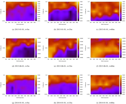
Taking the same three instances as Section V-A the parameter space is sampled at 54 points (initial temperature ∈ {1000, 1500, . . . ,5000}, cooling rate ∈ {0.0001,0.0005,0.001,0.0025, 0.005,0.01}. Each of these points in the parameter space is run with five seeds on each instance.

Figure 8 shows the best solution found by each of these configurations across the different runs at three time steps. The best parameter configuration varies across the different instances and also the run time of the algorithm. In general, the performance is more sensitive to cooling rate than initial temperature. Also high cooling rates allow the algorithm to find good solutions faster, while low cooling rates produce better solutions when given enough time. As there is no obvious way to predict the best configuration for particular input data a priori we now investigate the parallel execution of a portfolio of configurations to attain robustness across varied input data.

C. Cloud deployment

This section demonstrates that distributing a portfolio of solvers in the cloud allows the quality of constructed schedules to scale with the computational resources invested in the problem. As seen in Section V-A simulated annealing con-sistently outperforms hill climbing so we focus our attention on a portfolio of simulated annealing algorithms. As shown in Section V-B the quality of the best constructed schedule is heavily dependent on the configuration of the algorithm, but the best setting varies across instances. There is no easy way to determine the best configuration for an instance a priori, so our portfolio contains a variety of configurations. Also as highlighted in Section V-A, the performance of the algorithm is also dependant on the seed, so our portfolio is extended to include multiple seeds for each solver configuration.

66000 66500 67000 67500 68000 68500 69000 69500 70000 70500 71000

0 10 20 30 40 50 60

Gain

Time (m)

HC1 HC2 SA

(a) 2013-01-01 - Mean

66000 66500 67000 67500 68000 68500 69000 69500 70000 70500 71000

0 10 20 30 40 50 60

Gain

Time (m)

HC1 HC2 SA

(b) 2013-01-01 - Best

385000 390000 395000 400000 405000 410000 415000 420000

0 10 20 30 40 50 60

Gain

Time (m) HC1

HC2 SA

(c) 2013-06-01 - Mean

385000 390000 395000 400000 405000 410000 415000 420000

0 10 20 30 40 50 60

Gain

Time (m)

HC1 HC2 SA

(d) 2013-06-01 - Best

79000 79500 80000 80500 81000 81500 82000 82500

0 10 20 30 40 50 60

Gain

Time (m)

HC HC2 SA

(e) 2014-01-01 - Mean

79000 79500 80000 80500 81000 81500 82000 82500

0 10 20 30 40 50 60

Gain

Time (m)

HC1 HC2 SA

(f) 2014-01-01 - Best

(a) 2013-01-01, t=5m (b) 2013-01-01, t=15m (c) 2013-01-01, t=60m

(d) 2013-06-01, t=5m (e) 2013-06-01, t=15m (f) 2013-06-01, t=60m

(g) 2014-01-01, t=5m (h) 2014-01-01, t=15m (i) 2014-01-01, t=60m

Fig. 8. A parameter sweep for the simulated annealing algorithm using neighbourhood NH2 across three historical instances at three time steps. Clearly the best configuration depends on the problem instance as well as the length of time the algorithm will be run. It is not possible to choose a globally optimal configuration for all possible input data or expected run times.

is supported by the MIT StarCluster for managing the AWS resources. Ten c4.8xlarge4 VMs with 36 vCPUs and 60 GB memory was employed.

By re-sampling the results from this portfolio we are able to demonstrate how the quality of the best schedule scales with both the number of configurations and the number of seeds per configuration. In order to normalise the results across the different instances, the result of GREEDYwas mapped to 0 and the best solution found across the portfolio was mapped to one. Intermediate values are determined via linear interpolation.

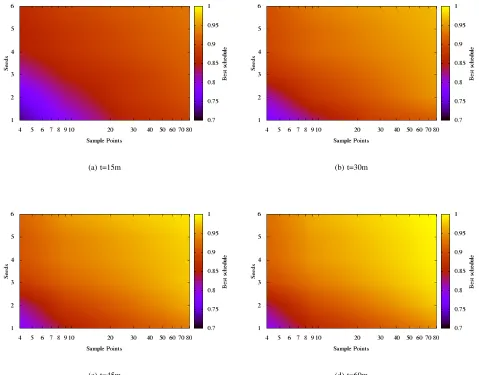
The results are shown in Figure 9. It is clear that the quality of the best schedule found at each of the time steps increases

4_{http://aws.amazon.com/ec2/instance-types/}

(a) t=15m (b) t=30m

(c) t=45m (d) t=60m

Fig. 9. The results of deployment of the e-Infrastructure on cloud virtual machines averaged across ten historical instances. By increasing either the number of algorithm configurations or runs per configuration we increase the quality of the best schedule found. This scalability in performance is observed up to 486 vCPUs. Also scaling the amount of available resources improves the performance of the algorithm at all time steps so the anytime performance of the algorithm has been improved.

VI. CONCLUSION

In this paper, we have presented a cloud-based e-Infrastructure to schedule microlensing observation. To achieve this we proposed a quality metric for microlensing ob-servation schedules that adequately accounts for rescheduling after interrupted observations along with several techniques for constructing high quality schedules by the application of local search techniques including hill climbing and simulated annealing. Experimental investigation found that given the correct configuration simulated annealing was the most ef-fective strategy. The experimental studies performed on the Amazon cloud demonstrated robust performance when a large pool of computational resource were used for implementing these techniques and executing them across varied input data. The results reported in this paper ascertain that such a

cloud-based e-Infrastructure is an ideal solution towards efficiently generating observation schedules given that the computational requirements for rescheduling are both bursty and highly unpredictable.

In the future, efforts will be made towards deploying the e-Infrastructure in real-time. We aim to explore the under-lying methods in the context of multiple telescopes as well as incorporating techniques for load balancing and dynamic rescheduling of resources on the cloud.

ACKNOWLEDGMENT

REFERENCES

[1] A. Einstein, “Lens-like action of a star by the deviation of light in the gravitational field,”Science, vol. 84, no. 2188, pp. 506–507, 1936. [2] B. Paczynski, “Gravitational microlensing by the galactic halo,” The

Astrophysical Journal, vol. 304, pp. 1–5, 1986.

[3] S. Mao and B. Paczynski, “Gravitational microlensing by double stars and planetary systems,”The Astrophysical Journal, vol. 374, pp. L37– L40, 1991.

[4] M. Dominik, “Studying planet populations with einstein’s blip,” Philo-sophical Transactions of the Royal Society A: Mathematical, Physical and Engineering Sciences, vol. 368, no. 1924, pp. 3535–3550, 2010. [5] M. Kiraga and B. Paczynski, “Gravitational microlensing of the galactic

bulge stars,”The Astrophysical Journal, vol. 430, pp. L101–L104, 1994. [6] A. Gould and A. Loeb, “Discovering planetary systems through gravita-tional microlenses,”The Astrophysical Journal, vol. 396, pp. 104–114, 1992.

[7] M. Dominik, M. Albrow, J.-P. Beaulieu, J. Caldwell, D. DePoy, B. Gaudi, A. Gould, J. Greenhill, K. Hill, S. Kaneet al., “The planet microlensing follow-up network: results and prospects for the detection of extra-solar planets,”Planetary and Space Science, vol. 50, no. 3, pp. 299–307, 2002.

[8] M. Dominik, N. Rattenbury, A. Allan, S. Mao, D. Bramich, M. Burgdorf, E. Kerins, Y. Tsapras et al., “An anomaly detector with immediate feedback to hunt for planets of earth mass and below by microlensing,” Monthly Notices of the Royal Astronomical Society, vol. 380, no. 2, pp. 792–804, 2007.

[9] I. Bond, F. Abe, R. Dodd, J. Hearnshaw, M. Honda, J. Jugaku, P. Kilmartin, A. Marles, K. Masuda, Y. Matsubaraet al., “Real-time difference imaging analysis of moa galactic bulge observations during 2000,” Monthly Notices of the Royal Astronomical Society, vol. 327, no. 3, pp. 868–880, 2001.

[10] A. Udalski, “The optical gravitational lensing experiment. real time data analysis systems in the ogle-iii survey,”Acta Astronautica, 2003. [11] M. Mora and M. Solar, “A survey on the dynamic scheduling

problem in astronomical observations,” in Artificial Intelligence in Theory and Practice III, ser. IFIP Advances in Information and Communication Technology, M. Bramer, Ed. Springer Berlin Heidelberg, 2010, vol. 331, pp. 111–120. [Online]. Available: http://dx.doi.org/10.1007/978-3-642-15286-3 11

[12] M. Armbrust, A. Fox, R. Griffith, A. D. Joseph, R. H. Katz, A. Konwinski, G. Lee, D. A. Patterson, A. Rabkin, I. Stoica, and M. Zaharia, “Above the clouds: A berkeley view of cloud computing,” EECS Department, University of California, Berkeley, Tech. Rep. UCB/EECS-2009-28, Feb 2009. [Online]. Available: http://www.eecs.berkeley.edu/Pubs/TechRpts/2009/EECS-2009-28.html [13] I. Foster, Y. Zhao, I. Raicu, and S. Lu, “Cloud computing and grid

computing 360-degree compared,” in Grid Computing Environments Workshop, 2008. GCE ’08, Nov 2008, pp. 1–10.

[14] M. Dominik, K. Horne, A. Allan, N. Rattenbury, Y. Tsapras, C. Snod-grass, M. Bode, M. Burgdorf, S. Fraser, E. Kerins et al., “Artemis (automated robotic terrestrial exoplanet microlensing search): A possible expert-system based cooperative effort to hunt for planets of earth mass and below,”Astronomische Nachrichten, vol. 329, no. 3, pp. 248–251, 2008.

[15] M. Dominik, U. G. Jørgensen, N. Rattenbury, M. Mathiasen, T. Hinse, S. Calchi Novati, K. Harpsøe, V. Bozza, T. Anguita, M. Burgdorfet al., “Realisation of a fully-deterministic microlensing observing strategy for inferring planet populations,”Astronomische Nachrichten, vol. 331, no. 7, pp. 671–691, 2010.

[16] K. Horne, C. Snodgrass, and Y. Tsapras, “A metric and optimization scheme for microlens planet searches,”Monthly Notices of the Royal Astronomical Society, vol. 396, no. 4, pp. 2087–2102, 2009.

[17] S. J. Russell and P. Norvig,Artificial Intelligence: A modern approach, 2nd ed. Pearson Education, 1995.

[18] J. Pearl,Heuristics: Intelligent Search Strategies for Computer Problem Solving. Addison-Wesley Longman Publishing Co., Inc,, 1984. [19] S. Kirkpatrick, M. Vecchiet al., “Optimization by simmulated

anneal-ing,”Science, vol. 220, no. 4598, pp. 671–680, 1983.