The appearance, motion, and disappearance of three-dimensional magnetic null points
Nicholas A. Murphy, Clare E. Parnell, and Andrew L. Haynes
Citation: Physics of Plasmas 22, 102117 (2015); doi: 10.1063/1.4934929 View online: http://dx.doi.org/10.1063/1.4934929
View Table of Contents: http://scitation.aip.org/content/aip/journal/pop/22/10?ver=pdfcov Published by the AIP Publishing
Articles you may be interested in
Dynamics of charged particle motion in the vicinity of three dimensional magnetic null points: Energization and chaos
Phys. Plasmas 22, 032907 (2015); 10.1063/1.4916402
Magnetohydrodynamic study of three-dimensional instability of the spontaneous fast magnetic reconnection Phys. Plasmas 16, 052903 (2009); 10.1063/1.3095562
Current sheets at three-dimensional magnetic nulls: Effect of compressibility Phys. Plasmas 14, 052109 (2007); 10.1063/1.2734949
Current sheet formation and nonideal behavior at three-dimensional magnetic null points Phys. Plasmas 14, 052106 (2007); 10.1063/1.2722300
The appearance, motion, and disappearance of three-dimensional magnetic
null points
Nicholas A.Murphy,1,a)Clare E.Parnell,2and Andrew L.Haynes2 1
Harvard-Smithsonian Center for Astrophysics, Cambridge, Massachusetts 02138, USA 2
School of Mathematics and Statistics, University of St Andrews, North Haugh, St Andrews, Fife KY16 9SS, United Kingdom
(Received 14 September 2015; accepted 19 October 2015; published online 30 October 2015) While theoretical models and simulations of magnetic reconnection often assume symmetry such that the magnetic null point when present is co-located with a flow stagnation point, the introduc-tion of asymmetry typically leads to non-ideal flows across the null point. To understand this behavior, we present exact expressions for the motion of three-dimensional linear null points. The most general expression shows that linear null points move in the direction along which the magnetic field and its time derivative are antiparallel. Null point motion in resistive magnetohy-drodynamics results from advection by the bulk plasma flow and resistive diffusion of the mag-netic field, which allows non-ideal flows across topological boundaries. Null point motion is described intrinsically by parameters evaluated locally; however, global dynamics help set the local conditions at the null point. During a bifurcation of a degenerate null point into a null-null pair or the reverse, the instantaneous velocity of separation or convergence of the null-null pair will typically be infinite along the null space of the Jacobian matrix of the magnetic field, but with finite components in the directions orthogonal to the null space. Not all bifurcating null-null pairs are connected by a separator. Furthermore, except under special circumstances, there will not exist a straight line separator connecting a bifurcating null-null pair. The motion of separators cannot be described using solely local parameters because the identification of a particular field line as a separator may change as a result of non-ideal behavior elsewhere along the field line.
VC 2015 Author(s). All article content, except where otherwise noted, is licensed under a Creative
Commons Attribution 3.0 Unported License. [http://dx.doi.org/10.1063/1.4934929]
I. INTRODUCTION
Magnetic reconnection1–4 frequently occurs at and around magnetic null points: locations where the magnetic field strength equals zero.5–9 Magnetospheric null points have been identified using multipoint in situ measurements as the nulls pass through the spacecraft constellation.10–16 Null points in the solar atmosphere have been identified through extrapolation of the photospheric magnetic field and morphology in coronal emission.17–27Numerical simulations of magnetic reconnection and plasma turbulence at low guide fields frequently show the formation and evolution of null points,28,29as do numerical experiments of typical solar events such as flux emergence.30,31
Two-dimensional, non-degenerate magnetic null points are classified as X- or O-type depending on the local mag-netic field structure. If we defineMas the Jacobian matrix of the magnetic field at the null point, then a null point will be X-type if detM<0, O-type if detM>0, and degenerate if detM¼0. Magnetic reconnection in two dimensions can only occur at null points (e.g., Refs.32and33).
In three dimensions, the structure of non-degenerate magnetic null points is significantly more complex.5–9Null lines and null planes are structurally unstable and unlikely to exist in real systems (e.g., Refs. 7 and 34). The magnetic field structure around a linear three-dimensional null point
includes separatrix surfaces (or fans) of infinitely many field lines that originate (or terminate) at the null, and two spine field lines that end (or begin) at the null. A negative (or type A) null point has separatrix surface field lines heading inward toward the null point with spine field lines heading outward from the null point. In contrast, a positive (or type B) null point has separatrix surface field lines heading out-ward away from the null point and spine field lines heading inward toward the null point.
Separators (also known as X-lines by some in the mag-netospheric community) are magnetic field lines that connect two nulls. Separators that include a spine field line are not structurally stable, so separators in real systems will almost always be given by the intersection of two separatrix surfa-ces. Null points, separatrix surfaces, spines, and separators are the topological boundaries that divide the magnetic field into distinct domains and are therefore preferred locations for magnetic reconnection.31,35–37 Three-dimensional mag-netic reconnection can also occur without nulls,33,38–42 espe-cially in regions such as quasi-separatrix layers where the magnetic connectivity changes quickly.
Motion of magnetic null points and reconnection regions occurs during any realistic occurrence of magnetic reconnec-tion. In Earth’s magnetosphere, X-line retreat has been observed in the magnetotail43–46 and poleward of the cusp.47 At the dayside magnetopause48,49 and in tokamaks,50,51 the combination of a plasma-pressure gradient and a guide field leads to diamagnetic drifting of the reconnection site that can a)
1070-664X/2015/22(10)/102117/9 22, 102117-1 VCAuthor(s) 2015
suppress reconnection. Laboratory experiments frequently show reconnection site motion and asymmetry, often due to geometry or the Hall effect.52–55 During solar flares, the reconnection site often rises with time as the flare loops grow and can also show transverse motions (e.g., Refs.56and57).
Theoretical models of magnetic reconnection often assume symmetry such that each magnetic null coincides with a flow stagnation point in the reference frame of the system. When asymmetry is introduced, there is in general a separation between these two points,54,58–64 and in some cases a stagnation point might not even exist near a null point.65 In all of these situations, there will generally be plasma flow across the magnetic null and the null will change position. Interestingly, the velocity of a null point will generally not equal the plasma flow velocity at the null point.62–65 This effect is similar to the flow-through mode of reconnection.66,67 During asymmetric magnetic recon-nection in partially ionized plasmas, there may exist neutral flow through the current sheet from the weak magnetic field (high neutral pressure) side to the strong magnetic field (low neutral pressure) side due to the neutral pressure gradient.64
In previous work,62we derived an exact expression for the motion of an X-line when its location is constrained to one dimension by symmetry. In resistive magnetohydrody-namics (MHD), X-line motion results from a combination of advection by the bulk plasma flow and resistive diffusion of the normal component of the magnetic field. In this work, we present exact expressions for the motion of linear null points in three dimensions and discuss the typical prop-erties of the bifurcations of degenerate magnetic null points. SectionIIcontains a derivation of the motion of linear null points in a vector field. Section III uses the results from Section II to describe the motion of magnetic null points. Section IV considers the local bifurcation properties of magnetic null points and provides three examples. Section
V contains a summary of this work and discussion on the implications.
II. MOTION OF LINEAR NULL POINTS IN AN ARBITRARY VECTOR FIELD
We definexnðtÞas the time-dependent position of an iso-lated null point in a vector field Bðx;tÞ. We define BnðxnðtÞ;tÞas the value of the vector field at the null; while Bn0 for all time,@@BtjxnðtÞ
@Bn
@t 6¼0 when the null point is moving. We defineUto be the velocity of this null
Udxn
dt : (1)
The local structure of a non-degenerate null point can be found by taking a Taylor expansion and keeping the linear terms.5–9The linear structure is then given by
B¼Mdx; (2)
wheredxxxn. The elements of the Jacobian matrix M
evaluated at the null are given by
Mij¼@jBi; (3)
whereiis the row index andjis the column index. The trace ofMequals zero whenr B¼0, andM¼ ðrBÞT.
Next we take the derivative following the motion of the null
@Bn
@t þU rBjxn ¼0: (4)
This expression gives the total derivative of the magnetic field at the null point using the null’s velocity in an arbitrary refer-ence frame. This derivative equals zero because the magnetic field at the null by definition does not deviate from zero as we are following it. By solving forUin Eq.(4), we arrive at the most general expression for the velocity of the null point68–70
U¼ M1 @Bn
@t ; (5)
which is valid for vector fields of arbitrary dimension. This derivation provides an exact result as long as M is non-singular.
An alternate derivation for Eq. (5) starts from the first order Taylor series expansion of Bwith respect to time and space about a linear null point
Bðdx;dtÞ ¼Mdxþ@Bn
@t dtþ O kdxk
2
;dt2
: (6)
This first order expansion is valid in the limit of smalldtand
jdxj. We define dxn as the position of the null point at dt. Setting Bðdxn;dtÞ ¼0 provides a unique solution for Udxn=dt, and we again arrive at Eq.(5). Unlike the previ-ous paragraph, this derivation uses the linearization approxi-mation. Eq.(5)is related to the implicit function theorem.
Equation (5)shows that a null point will move along the path for which B and @Bn
@t are oppositely directed. The null point will move faster if the vector field is changing quickly in time or varying slowly in space along this path. This exact result forUcan be applied to find the velocity of linear null points in any time-varying vector field with con-tinuous first derivatives in time and space about the null point. A unique velocity U exists as long as M is non-singular. IfMis non-singular, then there exists exactly one radial path away from the null for which the vector field is pointed in a particular direction.
III. MOTION OF MAGNETIC NULL POINTS
We next consider the case where Bis a magnetic field rather than just any vector field. The derivation of Eq. (5)
does not invoke any of Maxwell’s equations. We now intro-duce Faraday’s law
@B
@t ¼ r E; (7)
whereEis the electric field. By combining Eqs.(5)and(7), we arrive at the relation
U¼M1ðr EÞ; (8)
which additionally requires continuous first derivatives of the electric field in space about the null point. This
expression does not depend on any particular Ohm’s law, and indeed can be applied in situations where there is no Ohm’s law.
Next we consider the resistive MHD Ohm’s law
EþVB¼gJ; (9)
whereVis the plasma flow velocity andJis the current den-sity. The resistivity gis assumed to be uniform for simplic-ity. Eq.(8)then becomes
U¼VgM1r2B; (10)
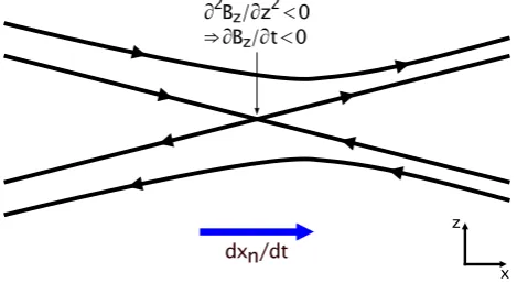
where all quantities on the right hand side are evaluated at the magnetic null. This expression requires thatBhas contin-uous first derivatives in time and contincontin-uous second deriva-tives in space about the null point. Null point motion in resistive MHD results from a combination of advection by the bulk plasma flow and resistive diffusion of the magnetic field. Even in the absence of flow, null points may still move in resistive situations. The plasma flow velocity at the null point does not equal the velocityofthe null point.62A sche-matic showing null point motion due to resistive diffusion is presented in Fig.1.
Equation (8) can also be evaluated using a generalized Ohm’s law containing additional terms.2 For example, we can use an Ohm’s law of the form
EþViB¼gJþ JB
ene
rpe
ene ; (11)
whereViis the bulk ion velocity,neis the electron density,e
is the elementary charge, andpeis a scalar electron pressure.
ForJ¼eneðViVeÞ, Eq.(8)becomes
U¼VegM1r2BþM1
rne rpe
n2
ee
; (12)
where quantities are again evaluated at the null point. The first term on the right hand side corresponds to the magnetic field being carried with the electron flow velocity,Ve, rather
than the bulk plasma flow; the second term corresponds to the resistive diffusion of the magnetic field at the null; and the third term corresponds to the Biermann battery.71,72
IV. THE APPEARANCE AND DISAPPEARANCE OF MAGNETIC NULL POINTS
We next consider the emergence and disappearance of magnetic null points, with an emphasis on the instantaneous velocity of separation or convergence of a bifurcating null-null pair. The local approach taken here complements global bifurcation studies.73Thus far we have just considered non-degenerate null points for which the local magnetic field can be described by Eq. (2) using only the linear terms in the Taylor series expansion. As long asMis non-singular at the null, then there exists a unique velocity corresponding to the motion of that null point. Non-degenerate null points are therefore structurally stable and cannot disappear unless M
becomes singular.68
In contrast, degenerate null points are structurally unsta-ble and generally exist instantaneously as a transition between different topological states.7,34 Null points must appear or disappear in oppositely signed pairs during a bifur-cation because the overall topological degree of the region cannot change unless a null point enters or leaves the domain across a boundary.74In most situations of physical interest, degenerate three-dimensional magnetic null points will have rankM¼2 and nullityM¼1 (e.g., Ref. 7). The null space (or kernel) of M will then be one-dimensional and corre-sponds to the eigenvector of M with eigenvalue zero. The three eigenvalues must sum to zero because of the diver-gence constraint,6which implies that the two non-zero eigen-values must either be both real and of opposite sign, or both complex and of opposite sign.9
Although the linear representation in Eq. (2) can describe the magnetic structure surrounding a degenerate null point (e.g., Ref.9) the region around a bifurcating null-null pair requires higher-order terms. Third-order terms need to be considered only when the first- and second-order deriv-atives both vanish at the null, so usually a second-order expansion will suffice. The Taylor series expansion of the magnetic field about a three-dimensional null point to second-order in time and space is
Bðdx;dtÞ ¼Mdxþ@Bn @t dtþ
1 2
dxTHxdx dxTH
ydx dxTHzdx
2 6 4
3 7 5
þdt
2
dx r
ð Þ@tBx
dx r
ð Þ@tBy
dx r
ð Þ@tBz
2 6 4
3 7 5þdt
2
2
@2B
n
@t2 þO kdxk 3
;dt3
;
(13)
[image:4.607.55.290.540.668.2]where the Jacobian matrix, Hessian matrices, and derivatives are evaluated at the null point. The elements of the Hessian matrices are given by Hk;ij¼@i@jBk for i;j;k2 fx;y;zg. If the magnetic field is locally continuous, then the partial de-rivative operators will be commutative and the Hessian mat-rices will be symmetric. When B_ is constant in time and space, then the fourth and fifth terms on the right hand side
FIG. 1. A two-dimensional example showing the motion of an X-type null point to the right (in the positivexdirection) due to resistive diffusion of the vertical component of the magnetic field (Bz) along the vertical (z) direction.
Above and below the null, Bz<0. The negativeBzdiffuses along the z
direction into the immediate vicinity of the null point. At a slightly later time, the magnetic field at the current position of the null point will have
Bz<0. The negativeBzdiffusion cancels out positiveBzto the right of the
null point, so the resulting null point motion is to the right. Reproduced with permission from Phys. Plasmas 17, 112310 (2010). Copyright 2010 American Institute of Physics.
of Eq. (13) vanish. The positions of the null points for a givendtmay be found by settingBðdxn;dtÞ ¼0 in Eq.(13) (or the full expression of the magnetic field) and then solving fordxn.
The instantaneous velocity of convergence or separation of a bifurcating null-null pair may be infinite, finite, or zero (see SectionIV Afor examples). Suppose that there exists a degenerate three-dimensional null point with rankM¼2 and thatM has three unique eigenvectors. The first-order direc-tional derivatives of each component ofBare zero along the one-dimensional null space of M. Under most realistic cir-cumstances, the second-order directional derivative of B along the null space ofMwill be nonzero. Except in special circumstances, the component of velocity along the null space ofMof the bifurcating null-null pair will be instanta-neously infinite. Next, consider the two-dimensional sub-space that is orthogonal to the null sub-space ofM. The Jacobian of M in this subspace at the null point will be invertible. Consequently, there exists a unique finite velocity within this subspace for the two-dimensional null point. Thus, in gen-eral, the instantaneous component of velocity along the null space of a bifurcating null-null pair will be infinite while the components of velocity orthogonal to the null space will be finite or zero.
Next we consider separators that may exist and connect a bifurcating null-null pair. Because these bifurcations can-not change the topological degree of the system, the null-null pair will include one negative null-null and one positive null.7,74DefineR andRþ as the separatrix surfaces andc
and cþ as the spine field lines of the negative and positive
null points, respectively. The field lines in R and cþ
approach the null, while the field lines inRþ andcrecede
from the null. In the neighborhood of a linear null, the sepa-ratrix surface is given by the plane spanned by the two eigen-vectors associated with eigenvalues that have the same sign for their real part, and the two spine field lines are along the remaining eigenvector.9
Separators that exist in real systems will almost always be given by the intersection of two separatrix surfaces.7,36 Spine-spine separators may exist if c and cþ include the
same field line. Though spine-spine separators may occur in some symmetric systems, they are not structurally stable and thus can generally be ignored.36As explained above, during the bifurcation of a degenerate null point a positive and neg-ative null are formed; hence, spine-fan separators can never connect a bifurcating null-null pair because such separators connect either two positive or two negative nulls. Additionally, not all bifurcating null-null pairs will be con-nected by a separator.
In most realistic situations, there will not exist a straight line separator connecting a bifurcating null-null pair as one might intuitively expect (see also Refs.7and8). Typically, there will exist some angle between the separatrix surfaces of each of the two null points in the time surrounding the bifurcation. Equivalently, each pair of eigenvectors associ-ated with the separatrix surface of each null will usually be changing in time, and, in general, this evolution will be dif-ferent for each separatrix surface.
A straight line separator may only be created under spe-cial circumstances, such as when certain symmetries are
present. For example, a straight line separator will occur if the two nulls from the bifurcating null-null pair are both improper nulls (not spiral) and they both share the same fan eigenvector which is parallel to the direction of motion of the bifurcating nulls.
A. Bifurcation examples
Let us consider a prototypical null point bifurcation of the form
Bðx;tÞ ¼
ðazÞxþby
cx ðaþzÞy z2
2 4
3
5þdBðx;tÞ; (14)
where a, b, and c are arbitrary real constants with a2þbc6¼0. We assume that dBðx;0Þ ¼0 so that there exists a degenerate null point at the origin with rankM¼2 att¼0. The null space ofMat the degenerate null point is given by^z, which is the eigenvector of Mcorresponding to eigenvalue zero. The remaining eigenvectors of the degener-ate null point are in thex-yplane and given by
e1
b
aþpffiffiffiffiffiffiffiffiffiffiffiffiffiffiffia2þbc
0
2 4
3
5ande2
b
apffiffiffiffiffiffiffiffiffiffiffiffiffiffiffia2þbc
0
2 4
3 5; (15)
which correspond to eigenvalues ða2þbcÞ and a2þbc,
respectively. We only consider time and space close to the bifurcation such thatjdBzj<ja2þbcj. These examples will
elucidate many of the properties of null point bifurcations discussed earlier in this section.
1. First bifurcation example
Suppose that dBðtÞ ¼ ^zsgnðtÞjtja in Eq. (14). We assume thata>0 so that the expression fordBðtÞdoes not diverge near t¼0. For t>0, the third component of B reduces toz2ta and two null points exist, but whent<0,
there are no null points. At t¼0, a single second-order null point appears at the origin as the system undergoes a saddle-node bifurcation. For t>0, the two null points are at xn¼ ½0;0;6ta=2>. The null point withzn>0 will be a posi-tive null if a2þbc>0 and a negative null otherwise. The null points have velocities of x_n¼ ½0;0;6a2ta=21>. When 0<a<2, the velocity of separation diverges to infinity at t¼0. For the critical case whena¼2, the null point veloc-ities are constant: x_n ¼ ½0;0;61>. When a>2, the null point velocities asymptotically approach zero att¼0. Since the null point velocities are purely in the^zdirection and this is also the direction of an eigenvector of the fan planes of each of the nulls, the resulting separator is a straight line alongx¼y¼0 for whichBz<0.
Finely tuned examples such as this one are unlikely to occur in nature, but show that instantaneous velocities that are infinite, finite, or zero are mathematically allowable dur-ing the bifurcation of a degenerate null point.
2. Second bifurcation example
Suppose thatdBðtÞ ¼B_tin Eq.(14), whereBx_ ; By_ , and
_
Bz are real constants with Bz_ <0. By setting Bðxn;tÞ ¼0,
we arrive at this expression for the null point positions for
t0,
xnð Þ ¼t
aBxt_ bByt_ 7Bx_ pffiffiffiffiffiffiffiffiffiBz_ t3=2 a2þbcþBzt_
cBxt_ þaByt_ 7By_ pffiffiffiffiffiffiffiffiffiBz_ t3=2 a2þbcþBzt_
6pffiffiffiffiffiffiffiffiffiffiBzt_
2 6 6 6 6 6 6 6 6 4
3 7 7 7 7 7 7 7 7 5
: (16)
The instantaneous velocities of the bifurcating null points at t¼0 are given by
lim
t!0þx_nð Þ ¼t
aBx_ bBy_
a2þbc
cBx_ þaBy_
a2þbc
61 2
6 6 6 6 6 6 4
3 7 7 7 7 7 7 5
: (17)
The velocity in thex-y plane will be finite except under the special circumstance when Bx_ ¼By_ ¼0 in which case the velocity in the x-y plane will be zero. The instantaneous component of velocity along the null space ofMis infinite.
The eigenvectors, eigenvalues, and direction normal to the fan for the null points resulting from the bifurcation are shown in TableI. The eigenvectors associated with each null are not functions of time for this example, but the eigenval-ues are. The structure of the resulting null-null pair depends on the value ofa2þbc.
When a2þbc>z2
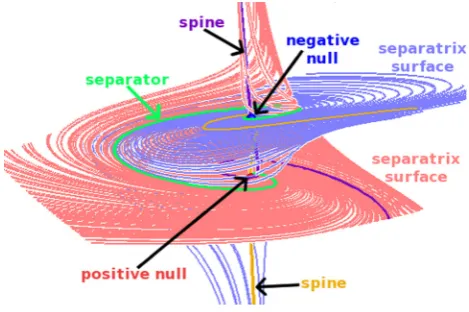
n>0 (case 1), all eigenvalues are real so the bifurcation results in a positive improper null point with zn>0 and a negative improper null point with zn<0. The separatrix surfaces cannot be parallel in such a case, so a separator exists between the two nulls as the curved intersection of the two separatrix surfaces (see Figure
2for a typical example).
Whena2þbc<0 (case 2), each null has two complex conjugate eigenvalues so the bifurcation results in a positive spiral null point withzn<0 and a negative spiral null point withzn>0. The field lines in the separatrix surfaces of both nulls are parallel to the x-yplane, so the separatrix surfaces do not intersect to yield a separator. A spine-spine separator can exist under special conditions (e.g., whenBx_ ¼By_ ¼0), but under generic conditions no separator will exist to con-nect these two newly formed null points. Figure3shows an example where the spine field lines of each null twist around each other before approaching the fan of the other null and spiraling away.
A separator will exist as a straight line between the two bifurcating null points if and only if Bx_ ¼By_ ¼0 for both case 1 and case 2.
3. Third bifurcation example
[image:6.607.48.560.67.166.2]In contrast to the first two examples, we now consider a magnetic field perturbation that is a function of both time and space. From Eq. (14), we define dBðx;tÞ ¼ ½Bxt_ ;Byt_ ;3yt2t> whereBx_ andBy_ are real constants. For
TABLE I. The eigenvectors, eigenvalues, and direction normal to the fan for the null points in the second bifurcation example.
Case 1:a2þbc>z2
n>0 Case 2:a2þbc<0
Pos. null (zn>0) Neg. null (zn<0) Pos. null (zn<0) Neg. null (zn>0)
Fan eigenvector, eigenvalue ^z;2jznj ^z;2jznj e1;jznj þ
ffiffiffiffiffiffiffiffiffiffiffiffiffiffiffi
a2þbc p
e1;jznj
ffiffiffiffiffiffiffiffiffiffiffiffiffiffiffi
a2þbc p
Fan eigenvector, eigenvalue e2;jznj þ
ffiffiffiffiffiffiffiffiffiffiffiffiffiffiffi
a2þbc p
e1;jznj
ffiffiffiffiffiffiffiffiffiffiffiffiffiffiffi
a2þbc p
e2;jznj
ffiffiffiffiffiffiffiffiffiffiffiffiffiffiffi
a2þbc p
e2;jznj þ
ffiffiffiffiffiffiffiffiffiffiffiffiffiffiffi
a2þbc p
Spine eigenvector, eigenvalue e1;jznj
ffiffiffiffiffiffiffiffiffiffiffiffiffiffiffi
a2þbc p
e2;jznj þ
ffiffiffiffiffiffiffiffiffiffiffiffiffiffiffi
a2þbc p
^
z;2jznj z^;2jznj
Direction normal to fan ½aþpffiffiffiffiffiffiffiffiffiffiffiffiffiffiffia2þbc;b;0>
[image:6.607.319.553.544.688.2]½apffiffiffiffiffiffiffiffiffiffiffiffiffiffiffia2þbc;b;0> ^z ^z
FIG. 2. Two improper null points (red and blue spheres) resulting from the bifurcation of a degenerate null point with a2þbc>z2
n>0 (case 1 in
SectionIV A 2). The fan surfaces of the two nulls (denoted by salmon field lines for the positive null atzn>0 and light blue field lines for the negative
null atzn<0) intersect to yield a curved separator field line (green). The
[image:6.607.56.289.572.697.2]spine field lines are orange (purple) for the positive (negative) null. In this example,ða;b;cÞ ¼ ð2;1;3Þ;B_ ¼ ½1;1;1>, andt¼0.2.
FIG. 3. Two spiral null points (red and blue spheres) resulting from the bifur-cation of a degenerate null point witha2þbc<0 (case 2 in SectionIV A 2).
The spine field lines [thick red (dark blue) lines for the positive (negative) nulls] wrap around each other instead of intersecting. The fan surfaces [salmon (light blue) lines for the positive (negative) nulls] are parallel to each other and thex-yplane, and do not intersect. Hence, no separator connects this bifur-cating null-null pair. In this example,ða;b;cÞ ¼ ð1;1;2Þ;B_ ¼ ½1;1;2>, andt¼0.1.
the particular case shown in Figure4,ða;b;cÞ ¼ ð1;1;2Þ. A separator is created connecting the bifurcating null-null pair because both the eigenvalues and eigenvectors of the nulls evolve in time. The separators formed in the case between two bifurcating spiral nulls are typically long and highly spiraled. Solving for B¼0 using the above values in Eq.(14)gives the following as the null point locations as a function oft:
xnð Þ ¼t
1
2 16
ffiffiffiffiffiffiffiffiffiffiffiffiffiffiffiffiffiffi
2t3tyn
p
yn yn
6pffiffiffiffiffiffiffiffiffiffiffiffiffiffiffiffiffiffi2t3tyn
2 6 6 4
3 7 7
5; (18)
where yn¼ ½ð1þ2tÞ þp28tffiffiffiffiffiffiffiffiffiffiffiffiffiffiffiffiffiffiffiffiffiffiffiffiffiffi2þ4tþ1=6t. In the limit of
t!0, we must consider the quadratic equation satisfied by yn,
3ty2n ð1þ2tÞyn2t¼0; (19)
which implies yn¼0 (and, hence, xn¼zn¼0) as t!0.
Differentiating this quadratic with respect totand then tak-ing the limit t!0 reveals that y_n¼ 2. It can then be shown that in the limitt!0, the instantaneous velocities of the bifurcating null points arex_n ¼ ½1;2;61>.
V. DISCUSSION
In this paper, we derive an exact expression for the motion of linear null points in a vector field and apply this expression to magnetic null points. Resistive diffusion and other effects in the generalized Ohm’s law allow for non-ideal flows across magnetic null points. In resistive MHD, null point motion results from a combination of advection by the bulk plasma flow and resistive diffusion of the magnetic field. These results are particularly relevant to studies of null point magnetic reconnection, especially when asymmetries are present. Analytical models of asymmetric reconnection must necessarily satisfy these expressions. Non-ideal flows at null points allow the transfer of plasma across topological boundaries.
Just as we must be careful when describing the motion of magnetic field lines,75–77 we must also be careful when describing the motion of magnetic null points. Null points are not objects. A null point is not permanently affixed to a parcel of plasma except in ideal or certain perfectly symmet-ric cases. Null points cannot be pushed directly by plasma pressure gradients or other forces on the plasma, but there will generally be indirect coupling between the momentum equation and Faraday’s law that contributes to null point motion. The motion of a null point is determined intrinsically by local quantities evaluated at the null point. However, global dynamics help set the local conditions that determine null point motion.
In addition to providing insight into the physics of non-ideal flows at magnetic null points and constraining models of asymmetric reconnection, the expressions for null point motion have several practical applications. Locating nulls of vector fields in three dimensions is non-trivial,78,79but if the null point positions are found for one time, then these expressions provide a method for estimating the positions of null points at future times. When there exists a cluster of sev-eral null points, these expressions provide a method for iden-tifying which null points correspond to each other at different times. A practical limitation is that these expres-sions will often require evaluating derivatives of noisy or nu-merical data (cf. Refs. 80 and 81). However, these expressions provide a test of numerical convergence and can be used to estimate the effective numerical resistivity in simulations of null point reconnection (compare to Refs.82
and83).
Linear magnetic null points appear and disappear in pairs associated with the bifurcation of a degenerate mag-netic null point. The null space of M in these degenerate nulls will typically be one-dimensional. Second or higher order terms in the Taylor series expansion are necessary to describe the structure of a degenerate null point and the region between a bifurcating null-null pair. Except in special circumstances, the instantaneous velocity of convergence or separation of a null-null pair will typically be infinite along the null space ofMbut with finite components of velocity in the orthogonal directions. This means that null-null pairs that have just appeared or are just about to disappear will not lie next to one another, but will always have a finite separation no matter how small a time step between frames is taken and regardless of whether the field is known numerically on a grid or analytically everywhere within a domain.
Just before or after a bifurcation, a straight line separator connecting the null-null pair will generally not exist. Furthermore, a separator, curved or straight, generic or non-generic, will not necessarily connect a null-null pair just before or after bifurcation if the nulls involved are of spiral type and their separatrix surfaces are parallel. The structures of second-order nulls and separators that exist very near a bifurcation remain important problems for future work.
In resistive MHD, null points must resistively diffuse in and out of existence. In the reference frame of the moving plasma, a necessary condition for a degenerate null point to form is that the resistive term in the induction equation, gr2B, be antiparallel to the magnetic field at the location of
[image:7.607.54.289.54.210.2]the impending degenerate null. This places physics-based
FIG. 4. As Figure3, but here the time derivative of thez-component of the magnetic field, B_z, is linear iny. The addition of a second-order term in
space and time means that the fan surfaces [salmon (light blue) lines for the positive (negative) nulls] tilt towards each other the instant after bifurcation creating a separator which connects this bifurcating null-null pair. In this example,ða;b;cÞ ¼ ð1;1;2Þ,t¼0.1, anddBðx;tÞ ¼ ½t;0;3yt2t>.
geometric constraints on when and where bifurcations are allowed to happen.
We may consider whether or not a similar local analysis can be performed to describe the motion of separators. Consider a separator that connects two magnetic null points. Suppose that a segment of this separator exhibits non-ideal evolution. Along the remainder of its length, the magnetic field in the vicinity of the separator evolves ideally. At a slightly later time, the field line that was the separator will, in general, not continue to be the separator between these two null points despite the locally ideal evolution. The motion of separators therefore cannot be described using solely local parameters. However, it may be possible to derive an expression for the motion of a separator by taking into account plasma flow and connectivity changes along its entire length. Such an approach would provide insight into the structural stability of separators and separator bifurca-tions,84as well as the nature of plasma flows across topologi-cal boundaries. This latter aspect is fundamental to the basic physics of three-dimensional reconnection; indeed, an early definition85states that reconnection is “the process whereby plasma flows across a surface that separates regions contain-ing topologically different magnetic field lines” (see also Ref. 39). We are investigating the problem of separator motion in two and three dimensions in ongoing work.
There exist numerous additional opportunities for future work. Our results take a local approach; consequently, nu-merical simulations are needed to investigate the interplay between local and global scales during null point motion and bifurcations. Numerical simulations can be used to investigate how null points diffuse in and out of existence in non-ideal plasmas and how separators behave during bifurca-tions. If the flow field and magnetic field are well diagnosed in space or laboratory plasmas, the expressions for null point motion may be used to provide constraints on magnetic field dissipation. Equation(10)offers another opportunity to mea-sure the plasma resistivity in the collisional limit. Dedicated laboratory experiments offer an opportunity to investigate plasma flow across null points (and other topological boun-daries) as well as null point and separator bifurcations. Finally, many results exist in the literature outside of plasma physics on bifurcations of vector fields and topology-based visualization of vector fields. While communication across disciplines is hindered by differences in terminology,86 the application of this external knowledge to plasma physics will likely lead to improved physics-based understanding of these processes.
ACKNOWLEDGMENTS
The authors thank A. Aggarwal, A. Bhattacharjee, A. Boozer, P. Cassak, J. Dorelli, T. Forbes, L. Guo, Y.-M. Huang, J. Lin, V. Lukin, M. Oka, E. Priest, J. Raymond, K. Reeves, C. Shen, V. Titov, D. Wendel, and E. Zweibel for helpful discussions. The authors thank A. Wilmot-Smith and D. Pontin for a discussion that helped elucidate why the motion of separators cannot be described locally. N.A.M. acknowledges the support from NASA grants NNX11AB61G, NNX12AB25G, and NNX15AF43G; NASA contract NNM07AB07C; and NSF SHINE grants
AGS-1156076 and AGS-1358342 to SAO. C.E.P. acknowledges support from the St Andrews 2013 STFC consolidated grant. This research has made use of NASA’s Astrophysics Data System Bibliographic Services. The authors thank the journal for publishing a manuscript containing only null results.
1
E. Priest and T. Forbes, Magnetic Reconnection: MHD Theory and Applications(Cambridge University Press, Cambridge, 2000).
2
Reconnection of Magnetic Fields: Magnetohydrodynamics and Collisionless Theory and Observations, edited by J. Birn and E. R. Priest (Cambridge University Press, Cambridge, 2007).
3E. G. Zweibel and M. Yamada, “Magnetic reconnection in astrophysical
and laboratory plasmas,”Annu. Rev. Astron. Astrophys.47, 291 (2009).
4M. Yamada, R. Kulsrud, and H. Ji, “Magnetic reconnection,”Rev. Mod.
Phys.82, 603 (2010).
5S. W. H. Cowley, “A qualitative study of the reconnection between the
Earth’s magnetic field and an interplanetary field of arbitrary orientation,”
Radio Sci.8, 903, doi:10.1029/RS008i011p00903 (1973).
6
S. Fukao, M. Ugai, and T. Tsuda, “Topological study of magnetic field near a neutral point,” RISRJ29, 133 (1975).
7
J. M. Greene, “Geometrical properties of three-dimensional reconnecting magnetic fields with nulls,” J. Geophys. Res. 93, 8583, doi:10.1029/ JA093iA08p08583 (1988).
8
Y.-T. Lau and J. M. Finn, “Three-dimensional kinematic reconnection in the presence of field nulls and closed field lines,”Astrophys. J.350, 672 (1990).
9C. E. Parnell, J. M. Smith, T. Neukirch, and E. R. Priest, “The structure of
three-dimensional magnetic neutral points,”Phys. Plasmas3, 759 (1996).
10C. J. Xiao, X. G. Wang, Z. Y. Pu, H. Zhao, J. X. Wang, Z. W. Ma, S. Y.
Fu, M. G. Kivelson, Z. X. Liu, Q. G. Zong, K. H. Glassmeier, A. Balogh, A. Korth, H. Reme, and C. P. Escoubet, “In situevidence for the structure of the magnetic null in a 3D reconnection event in the Earth’s magneto-tail,”Nat. Phys.2, 478 (2006).
11C. J. Xiao, X. G. Wang, Z. Y. Pu, Z. W. Ma, H. Zhao, G. P. Zhou, J. X.
Wang, M. G. Kivelson, S. Y. Fu, Z. X. Liu, Q. G. Zong, M. W. Dunlop, K.-H. Glassmeier, E. Lucek, H. Reme, I. Dandouras, and C. P. Escoubet, “Satellite observations of separator-line geometry of three-dimensional magnetic reconnection,”Nat. Phys.3, 609 (2007).
12J.-S. He, C.-Y. Tu, H. Tian, C.-J. Xiao, X.-G. Wang, Z.-Y. Pu, Z.-W. Ma,
M. W. Dunlop, H. Zhao, G.-P. Zhou, J.-X. Wang, S.-Y. Fu, Z.-X. Liu, Q.-G. Zong, K.-H. Glassmeier, H. Reme, I. Dandouras, and C. P. Escoubet, “A magnetic null geometry reconstructed from Cluster spacecraft observa-tions,”J. Geophys. Res.113, A05205, doi:10.1029/2007JA012609 (2008).
13D. E. Wendel and M. L. Adrian, “Current structure and nonideal behavior
at magnetic null points in the turbulent magnetosheath,”J. Geophys. Res. 118, 1571, doi:10.1002/jgra.50234 (2013).
14
R. Guo, Z. Pu, C. Xiao, X. Wang, S. Fu, L. Xie, Q. Zong, J. He, Z. Yao, J. Zhong, and J. Li, “Separator reconnection with antiparallel/component features observed in magnetotail plasmas,”J. Geophys. Res.118, 6116, doi:10.1002/jgra.50569 (2013).
15H. S. Fu, A. Vaivads, Y. V. Khotyaintsev, V. Olshevsky, M. Andre, J. B.
Cao, S. Y. Huang, A. Retino, and G. Lapenta, “How to find magnetic nulls and reconstruct field topology with MMS data?,”J. Geophys. Res.120, 3758, doi:10.1002/2015JA021082 (2015).
16
V. Olshevsky, A. Divin, E. Eriksson, S. Markidis, and G. Lapenta, “Energy dissipation in magnetic null points at kinetic scales,”Astrophys. J.807, 155 (2015).
17B. Filippov, “Observation of a 3D magnetic null point in the solar corona,”
Sol. Phys.185, 297 (1999).
18G. Aulanier, E. E. DeLuca, S. K. Antiochos, R. A. McMullen, and L.
Golub, “The topology and evolution of the Bastille day flare,”Astrophys. J.540, 1126 (2000).
19
H. Zhao, J.-X. Wang, J. Zhang, C.-J. Xiao, and H.-M. Wang, “Determination of the topology skeleton of magnetic fields in a solar active region,”Chin. J. Astron. Astrophys.8, 133 (2008).
20
D. W. Longcope and C. E. Parnell, “The number of magnetic null points in the quiet sun corona,”Sol. Phys.254, 51 (2009).
21
M. S. Freed, D. W. Longcope, and D. E. McKenzie, “Three-year global survey of coronal null points from potential-field-source-surface (PFSS) modeling and solar dynamics observatory (SDO) observations,”Sol. Phys. 290, 467 (2015).
22S. J. Edwards and C. E. Parnell, “Null point distribution in global coronal
potential field extrapolations,”Sol. Phys.290, 2055 (2015).
23S. Masson, E. Pariat, G. Aulanier, and C. J. Schrijver, “The nature of flare
ribbons in coronal null-point topology,”Astrophys. J.700, 559 (2009).
24
P. Demoulin, J. C. Henoux, and C. H. Mandrini, “Are magnetic null points important in solar flares?,” Astron. Astrophys.285, 1023 (1994).
25
G. Barnes, “On the relationship between coronal magnetic null points and solar eruptive events,”Astrophys. J. Lett.670, L53 (2007).
26R. M. Close, C. E. Parnell, and E. R. Priest, “Separators in 3D quiet-sun
magnetic fields,”Sol. Phys.225, 21 (2004).
27
S. Regnier, C. E. Parnell, and A. L. Haynes, “A new view of quiet-Sun to-pology from Hinode/SOT,”Astron. Astrophys.484, L47 (2008).
28
S. Servidio, W. H. Matthaeus, M. A. Shay, P. A. Cassak, and P. Dmitruk, “Magnetic reconnection in two-dimensional magnetohydrodynamic turbulence,”Phys. Rev. Lett.102, 115003 (2009).
29
S. Servidio, W. H. Matthaeus, M. A. Shay, P. Dmitruk, P. A. Cassak, and M. Wan, “Statistics of magnetic reconnection in two-dimensional magne-tohydrodynamic turbulence,”Phys. Plasmas17, 032315 (2010).
30
R. C. Maclean, C. E. Parnell, and K. Galsgaard, “Is null-point reconnec-tion important for solar flux emergence?,”Sol. Phys.260, 299 (2009).
31
C. E. Parnell, R. C. Maclean, and A. L. Haynes, “The detection of numer-ous magnetic separators in a three-dimensional magnetohydrodynamic model of solar emerging flux,”Astrophys. J.725, L214 (2010).
32
E. R. Priest, G. Hornig, and D. I. Pontin, “On the nature of three-dimensional magnetic reconnection,” J. Geophys. Res. 108, 1285, doi:10.1029/2002JA009812 (2003).
33
D. I. Pontin, “Three-dimensional magnetic reconnection regimes: A review,”Adv. Space Res.47, 1508 (2011).
34
G. Hornig and K. Schindler, “Magnetic topology and the problem of its invariant definition,”Phys. Plasmas3, 781 (1996).
35D. W. Longcope, “Topological methods for the analysis of solar magnetic
fields,”Living Rev. Sol. Phys.2, 7 (2005).
36
A. L. Haynes and C. E. Parnell, “A method for finding three-dimensional magnetic skeletons,”Phys. Plasmas17, 092903 (2010).
37
C. E. Parnell, A. L. Haynes, and K. Galsgaard, “Structure of magnetic sep-arators and separator reconnection,” J. Geophys. Res. 115, 2102, doi:10.1029/2009JA014557 (2010).
38
M. Hesse and K. Schindler, “A theoretical foundation of general magnetic reconnection,”J. Geophys. Res.93, 5559, doi:10.1029/JA093iA06p05559 (1988).
39
K. Schindler, M. Hesse, and J. Birn, “General magnetic reconnection, par-allel electric fields, and helicity,”J. Geophys. Res.93, 5547, doi:10.1029/ JA093iA06p05547 (1988).
40E. R. Priest and T. G. Forbes, “Magnetic flipping—reconnection in three
dimensions without null points,”J. Geophys. Res.97, 1521, doi:10.1029/ 91JA02435 (1992).
41G. Aulanier, E. Pariat, P. Demoulin, and C. R. DeVore, “Slip-running
reconnection in quasi-separatrix layers,”Sol. Phys.238, 347 (2006).
42
M. Janvier, G. Aulanier, E. Pariat, and P. Demoulin, “The standard flare model in three dimensions. III. Slip-running reconnection properties,”
Astron. Astrophys.555, A77 (2013).
43T. G. Forbes, E. W. Hones, S. J. Bame, J. R. Asbridge, G. Paschmann, N.
Sckopke, and C. T. Russell, “Evidence for the tailward retreat of a mag-netic neutral line in the magnetotail during substorm recovery,”Geophys. Res. Lett.8, 261, doi:10.1029/GL008i003p00261 (1981).
44
H. Hasegawa, A. Retino, A. Vaivads, Y. Khotyaintsev, R. Nakamura, T. Takada, Y. Miyashita, H. Re`me, and E. A. Lucek, “Retreat and reforma-tion of X-line during quasi-continuous tailward-of-the-cusp reconnecreforma-tion under northward IMF,” Geophys. Res. Lett. 35, L15104, doi:10.1029/ 2008GL034767 (2008).
45
M. Oka, T.-D. Phan, J. P. Eastwood, V. Angelopoulos, N. A. Murphy, M. Øieroset, Y. Miyashita, M. Fujimoto, J. McFadden, and D. Larson, “Magnetic reconnection X-line retreat associated with dipolarization of the Earth’s magnetosphere,”Geophys. Res. Lett.38, 20105, doi:10.1029/ 2011GL049350 (2011).
46
X. Cao, Z. Y. Pu, A. M. Du, V. M. Mishin, X. G. Wang, C. J. Xiao, T. L. Zhang, V. Angelopoulos, J. P. McFadden, and K. H. Glassmeier, “On the retreat of near-Earth neutral line during substorm expansion phase: A THEMIS case study during the 9 January 2008 substorm,”Ann. Geophys. 30, 143 (2012).
47
F. D. Wilder, S. Eriksson, K. J. Trattner, P. A. Cassak, S. A. Fuselier, and B. Lybekk, “Observation of a retreating x line and magnetic islands poleward of the cusp during northward interplanetary magnetic field conditions,” J. Geophys. Res. 119, 9643, doi:10.1002/2014JA020453 (2014).
48M. Swisdak, B. N. Rogers, J. F. Drake, and M. A. Shay, “Diamagnetic
suppression of component magnetic reconnection at the magneto-pause,” J. Geophys. Res. 108, 1218, doi:10.1029/2002JA009726 (2003).
49
T. D. Phan, G. Paschmann, J. T. Gosling, M. Oieroset, M. Fujimoto, J. F. Drake, and V. Angelopoulos, “The dependence of magnetic reconnection on plasmaband magnetic shear: Evidence from magnetopause observa-tions,”Geophys. Res. Lett.40, 11, doi:10.1029/2012GL054528 (2013).
50
B. Rogers and L. Zakharov, “Nonlinear x-stabilization of the m¼1
mode in tokamaks,”Phys. Plasmas2, 3420 (1995).
51M. T. Beidler and P. A. Cassak, “Model for incomplete reconnection in
sawtooth crashes,”Phys. Rev. Lett.107, 255002 (2011).
52
M. Inomoto, S. P. Gerhardt, M. Yamada, H. Ji, E. Belova, A. Kuritsyn, and Y. Ren, “Coupling between global geometry and the local Hall effect leading to reconnection-layer symmetry breaking,”Phys. Rev. Lett.97, 135002 (2006).
53
J. Yoo, M. Yamada, H. Ji, J. Jara-Almonte, C. E. Myers, and L.-J. Chen, “Laboratory study of magnetic reconnection with a density asymmetry across the current sheet,”Phys. Rev. Lett.113, 095002 (2014).
54
N. A. Murphy and C. R. Sovinec, “Global axisymmetric simulations of two-fluid reconnection in an experimentally relevant geometry,” Phys. Plasmas15, 042313 (2008).
55
V. S. Lukin and M. G. Linton, “Three-dimensional magnetic reconnection through a moving magnetic null,”Nonlinear Processes Geophys.18, 871 (2011).
56
T. G. Forbes and L. W. Acton, “Reconnection and field line shrinkage in solar flares,”Astrophys. J.459, 330 (1996).
57
S. L. Savage, D. E. McKenzie, K. K. Reeves, T. G. Forbes, and D. W. Longcope, “Reconnection outflows and current sheet observed with Hinode/XRT in the 2008 April 9 ‘Cartwheel CME’ flare,”Astrophys. J. 722, 329 (2010).
58P. A. Cassak and M. A. Shay, “Scaling of asymmetric magnetic
reconnec-tion: General theory and collisional simulations,” Phys. Plasmas 14, 102114 (2007).
59P. A. Cassak and M. A. Shay, “Scaling of asymmetric Hall magnetic
reconnection,” Geophys. Res. Lett. 35, 19102, doi:10.1029/ 2008GL035268 (2008).
60
P. A. Cassak and M. A. Shay, “Structure of the dissipation region in fluid simulations of asymmetric magnetic reconnection,” Phys. Plasmas 16, 055704 (2009).
61
N. A. Murphy, C. R. Sovinec, and P. A. Cassak, “Magnetic reconnection with asymmetry in the outflow direction,” J. Geophys. Res.115, 9206, doi:10.1029/2009JA015183 (2010).
62
N. A. Murphy, “Resistive magnetohydrodynamic simulations of X-line retreat during magnetic reconnection,”Phys. Plasmas17, 112310 (2010).
63
M. Oka, M. Fujimoto, T. K. M. Nakamura, I. Shinohara, and K.-I. Nishikawa, “Magnetic reconnection by a self-retreating X line,” Phys. Rev. Lett.101, 205004 (2008).
64
N. A. Murphy and V. S. Lukin, “Asymmetric magnetic reconnection in weakly ionized chromospheric plasmas,”Astrophys. J.805, 134 (2015).
65N. A. Murphy, M. P. Miralles, C. L. Pope, J. C. Raymond, H. D. Winter,
K. K. Reeves, D. B. Seaton, A. A. van Ballegooijen, and J. Lin, “Asymmetric magnetic reconnection in solar flare and coronal mass ejec-tion current sheets,”Astrophys. J.751, 56 (2012).
66
G. L. Siscoe, G. M. Erickson, B. U. Sonnerup, N. C. Maynard, J. A. Schoendorf, K. D. Siebert, D. R. Weimer, W. W. White, and G. R. Wilson, “Flow-through magnetic reconnection,”Geophys. Res. Lett.29, 4-1, doi:10.1029/2001GL013536 (2002).
67
N. C. Maynard, C. J. Farrugia, W. J. Burke, D. M. Ober, F. S. Mozer, H. Re`me, M. Dunlop, and K. D. Siebert, “Cluster observations of the dusk flank magnetopause near the sash: Ion dynamics and flow-through reconnection,”
J. Geophys. Res.117, A10201, doi:10.1029/2012JA017703 (2012).
68
J. M. Greene, “Reconnection of vorticity lines and magnetic lines,”Phys. Fluids B5, 2355 (1993).
69
T. Lindeberg, “Scale-space theory: A basic tool for analyzing structures at different scales,”J. Appl. Stat.21, 225 (1994).
70
T. Klein and T. Ertl, “Scale-space tracking of critical points in 3d vector fields,” in Topology-based Methods in Visualization, Mathematics and Visualization, edited by H. Hauser, H. Hagen, and H. Theisel (Springer, Berlin, Heidelberg, 2007) pp. 35–49.
71
L. Biermann, “Uber den Ursprung der Magnetfelder auf Sternen und im€ interstellaren Raum,” Z. Naturforschung5, 65 (1950); available athttp:// zfn.mpdl.mpg.de/data/Reihe_A/5/ZNA-1950-5a-0065.pdf.
72R. M. Kulsrud,Plasma Physics for Astrophysics (Princeton University
Press, Princeton, NJ, 2005).
73E. R. Priest, D. P. Lonie, and V. S. Titov, “Bifurcations of magnetic
topol-ogy by the creation or annihilation of null points,”J. Plasma Phys.56, 507 (1996); D. S. Brown and E. R. Priest, “Topological bifurcations in three-dimensional magnetic fields,”Proc. R. Soc. London, Ser. A 455, 3931 (1999); D. S. Brown and E. R. Priest, “The topological behaviour of 3D null points in the Sun’s corona,”Astron. Astrophys367, 339 (2001).
74
K. Deimling,Nonlinear Functional Analysis(Springer-Verlag, New York, 1985).
75
W. A. Newcomb, “Motion of magnetic lines of force,”Ann. Phys.3, 347 (1958).
76
D. P. Stern, “The motion of magnetic field lines,”Space Sci. Rev.6, 147 (1966).
77V. M. Vasyliunas, “Nonuniqueness of magnetic field line motion,”
J. Geophys. Res.77, 6271, doi:10.1029/JA077i031p06271 (1972).
78
J. M. Greene, “Locating three-dimensional roots by a bisection method,”
J. Comput. Phys.98, 194 (1992).
79A. L. Haynes and C. E. Parnell, “A trilinear method for finding null points
in a three-dimensional vector space,”Phys. Plasmas14, 082107 (2007).
80J. Cullum, “Numerical differentiation and regularization,” SIAM J.
Numer. Anal.8, 254 (1971).
81
R. Chartrand, “Numerical differentiation of noisy, nonsmooth data,”ISRN Appl. Math.2011, 164564.
82J. K. Edmondson, S. K. Antiochos, C. R. DeVore, B. J. Lynch, and T. H.
Zurbuchen, “Interchange reconnection and coronal hole dynamics,”
Astrophys. J.714, 517 (2010).
83C. Shen, J. Lin, and N. A. Murphy, “Numerical experiments on fine
struc-ture within reconnecting current sheets in solar flares,”Astrophys. J.737, 14 (2011).
84
D. S. Brown and E. R. Priest, “The topological behaviour of stable mag-netic separators,”Sol. Phys.190, 25 (1999).
85V. M. Vasyliunas, “Theoretical models of magnetic field line merging. I,”
Rev. Geophys. Space Phys.13, 303, doi:10.1029/RG013i001p00303 (1975).
86
Null points are also known as neutral points, fixed points, stationary points, equilibrium points, critical points, singular points, and singularities. Separators are also known as saddle connectors and separation/attachment lines. Separatrix surfaces are also known as fans and separation surfaces.