ISPRS International Journal of
Geo-Information
ISSN 2220-9964 www.mdpi.com/journal/ijgi/ Article
Impacts of Species Misidentification on Species Distribution
Modeling with Presence-Only Data
Hugo Costa 1,2,*, Giles M. Foody 1, Sílvia Jiménez 2 and Luís Silva 2
1 School of Geography, University of Nottingham, Nottingham, NG7 2RD, UK;
E-Mail: giles.foody@nottingham.ac.uk
2 InBIO—Associate Laboratoy, Research Network in Biodiversity and Evolutionary Biology,
Department of Biology, University of the Azores, 9501-801 Ponta Delgada, Azores, Portugal; E-Mails: tsire.85@gmail.com (S.J.); lsilva@uac.pt (L.S.)
* Author to whom correspondence should be addressed; E-Mail: lgxhag@nottingham.ac.uk or hugoagcosta@gmail.com; Tel.: +44-115-951-5428.
Academic Editors: Duccio Rocchini and Wolfgang Kainz
Received: 22 September 2015 / Accepted: 8 November 2015 / Published: 16 November 2015
Abstract: Spatial records of species are commonly misidentified, which can change the predicted distribution of a species obtained from a species distribution model (SDM). Experiments were undertaken to predict the distribution of real and simulated species using MaxEnt and presence-only data “contaminated” with varying rates of misidentification error. Additionally, the difference between the niche of the target and contaminating species was varied. The results show that species misidentification errors may act to contract or expand the predicted distribution of a species while shifting the predicted distribution towards that of the contaminating species. Furthermore the magnitude of the effects was positively related to the ecological distance between the species’ niches and the size of the error rates. Critically, the magnitude of the effects was substantial even when using small error rates, smaller than common average rates reported in the literature, which may go unnoticed while using a standard evaluation method, such as the area under the receiver operating characteristic curve. Finally, the effects outlined were shown to impact negatively on practical applications that use SDMs to identify priority areas, commonly selected for various purposes such as management. The results highlight that species misidentification should not be neglected in species distribution modeling.
Keywords: species mis-identification; false positive error; presence-only; MaxEnt
1. Introduction
Spatial patterns of species presence have been a central theme for long time in a variety of disciplines, such as ecology, biogeography, evolution, and management. Therefore, there is much interest in predicting the distribution of species, for which methods have been developed, including several modeling approaches widely known as species distribution models (SDMs) [1,2]. Typically, SDMs relate spatially-limited records of the presence or abundance of a species to environmental variables (e.g., temperature) that control its distribution. The relationships established may then be used to predict the presence of the species across unsurveyed areas [3].
Error and uncertainty abound in SDM-based analysis. Barry and Elith [4] classify the sources of error and uncertainty embedded in SDMs into two main categories: deficiencies in the data and deficiencies introduced by the specification of the model. In the first category, common problems include missing variables [4], small sample size [5,6], biased samples [7], incorrectly located species records [6], lack of absence records [8], and disagreement between the scale (grain/extent) of the species data and the modeling setup [1,6,9]. The second category includes possible discrepancies between the model used and the “true” model (e.g., if the model used is linear and the true relationship between species presence and variables is quadratic) and the modeling approach (e.g., envelope, distance-based, and regression) [4].
In this paper, attention is focused on the deficiencies in data, namely the species data. The quality of species data is often compromised for a variety of reasons. For example, commonly used datasets, such as those obtained from museums, herbariums, and atlases, often include only presence records (i.e., spatial reference where the species was detected), frequently resulting from ad hoc compilations of records collected occasionally without information on the species’ absence and survey effort; the latter is relevant since easily-accessible areas (e.g., near roads) are often more surveyed than remote areas, which leads to spatially-biased samples [8,10].
A variety of impacts of species data deficiencies on SDMs have been studied and a range of mitigation solutions have been proposed. For example, modeling methods have been developed that use presence-only data [11]; the impact of limited sample size in modeling have been studied [5,12]; and solutions have been proposed for the problem of incorrectly located species records [13], uneven sampling effort [14–16], spatial autocorrelation [17–20], and scales [21,22]. However, not all deficiencies in species data sets have been fully studied. One key problem that has attracted little attention yet may be common is that of species misidentification. Species misidentification is a particular type of false positive error, which occurs when a species is recorded as being present at a location where it is in fact absent. An example of a false positive error other than species misidentification is double-counting of individuals (e.g., when aural point counts are used to detect birds [23]). Here, the concern is when a species is simply misidentified.
sharks [26], 23% for hawks [27], ∼27% for freshwater mussels [28], and ∼70% for robber flies [29]. The magnitude of the problem of species misidentification varies as a function of several factors, namely the surveyor’s level of expertise and the species involved. For example, in a study addressing the causes of species misidentification in vegetation monitoring, Scott and Hallam [30] found an average misidentification rate of 2.7%–25.6% depending on surveyors’ expertise. Furthermore, Scott and Hallam [30] found high misidentification rates (e.g., >14%) for specific categories of plants, such as lower plants and particular trees.
A rare example of a study that addressed the impacts of species misidentification on research using SDMs is that of Ensing, et al. [31] in a study that predicted the potential distribution of an invasive species in North America. Ensing, et al. [31] found that the species distribution modeled using all of the presence records available (possibly including misidentifications) was substantially larger than that based only on records regarded as taxonomically “reliable”. A similar conclusion is drawn by Molinari-Jobin, et al. [32] using reliable and non-reliable data to predict the distribution of the Eurasian lynx in the Alps with site-occupancy modeling.
The effects of species misidentification on studies using SDMs are, however, still to be fully understood. A key issue is whether the misidentification committed is arbitrary or systematic. Arbitrary misidentification refers here to errors that lack a clear pattern, specifically, when the source of error vary. For example, the presumed presence of a species may involve confusion with several species, recorded by different surveyors with different expertise, and following inconsistent methodologies [31,32]. Systematic misidentification refers to the systematically confusion of one species with another. Systematic species misidentification can happen especially when two species are both morphologically similar and sympatric. For example, misidentifications of white marlin (Tetrapturus albidus) have occurred for a long time with the morphologically similar and sympatric roundscale spearfish (T. georgii); as a result, the two species were unknowingly assessed and managed as a species group [33].
2. Material and Methods
[image:4.595.83.511.318.694.2]To explore the effects of species misidentification error on species distribution modeling, a series of analyses were undertaken. The analyses focused on the effects of misidentification error on the predicted distribution of a species of interest and its potential impact on practical applications that use SDMs to select regions for various purposes such as management of endangered species. Specifically, four analyses were performed in which the modeling results obtained with data regarded as a gold standard (i.e., error-free) were compared to the results obtained with data contaminated with misidentification error. To ensure that the misidentification error could be known and characterized accurately to enable a rigorous assessment of the impacts of species misidentification on modeling a set of simulated datasets were used, but a real dataset is also used to provide an illustrative case study of the importance of the topic. Six rates, r, of species misidentification (contamination) were used: 1, 2, 4, 8, 16, and 32%; all inside the range of values reported in the literature highlighted above. All analyses were undertaken using a widely used species distribution model: maximum entropy (MaxEnt) [11].
2.1. Real Data
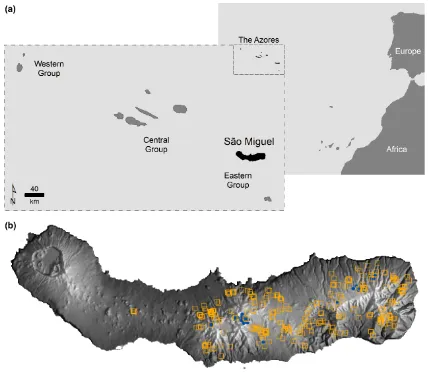
The real data used in this study relate to the island of São Miguel in the Azores (Portugal). The Azores is an archipelago of volcanic origin located in the North Atlantic Ocean, about 1500 km west from mainland Portugal (Figure 1a). The Azorean climate is temperate oceanic with a mean annual temperature of 17 °C at sea level, decreasing with altitude. Relative humidity is high and rainfall ranges from 1000 to well above 3000 mm yr−1, increasing with altitude and from east to west [34,35].
São Miguel is the largest island (745 km2), and its highest peak stands 1103 m high in the East (Figure 1b).
The real species data used were collected in a field survey conducted between September 2011 and May 2012 across São Miguel in order to increase the knowledge about the presence of tree ferns, which are alien to the Azores. The presence of tree ferns was detected during field surveys undertaken by car and on foot. Thus, the species datasets resulted from ad hoc compilations of records collected occasionally without information on the species’ absence and survey effort.
The species of interest (hereafter referred to as target species) is Cyathea cooperi (351 individuals recorded). C. cooperi is a tree fern considered as problematic because of its invasiveness [36] and is one of the top 100 invasive alien species with management priority in European Macaronesia [34]. C. cooperi can be confused with C. medullaris, which was identified for the first time in the Azores in the 2011/2012 survey (32 records). These two species are morphologically similar, with a further 141 records labeled only as Cyathea sp. as their exact species was not clear. Finally, samples of another tree fern species, Dicksonia antartica, were obtained (59 individuals recorded) which could be useful in modeling.
The presence of C. medullaris casts doubts upon past studies on the presence of C. cooperi in São Miguel because misidentifications may have happened historically. The situation is particularly possible because of the high number of specimens identified as C. medullaris in an apparently self-supporting population, which makes it unlikely that it was introduced recently. The presence of C. cooperi was recorded in a range of environments while C. medullaris was less dispersed geographically. In particular, C. medullaris was mainly observed at high altitude while C. cooperi was observed at all altitudes (Figure 1b). Note there are no guaranties the datasets of C. cooperi and C. medullaris are free of misidentification error. All specimens difficult to identify were labeled as Cyathea sp. but errors may have been made. For practical reasons, in this paper these data sets were used as if there were no error.
and the position of the Sun (the winter and summer solstices were considered). Curvature is the second derivative of the surface, thus highlighting flat, convex, and concave areas. These variables were used as indicators of local environmental conditions known to affect plant species distribution that were not available for this study, such as available soil water and insolation.
2.2. Simulated Data
Real species datasets are typically flawed in some fashion, specifically in relation to issues, such as data quality and sampling bias. Hence, to further illustrate the importance of species misidentification on SDMs predictions, simulated species data were generated with well-defined characteristics. A target species and a contaminating species were simulated as being at equilibrium with the environment, that is, the species were defined as present at all locations ecologically suitable, thus satisfying the equilibrium assumption of most SDMs [1,3].
The environmental suitability for the presence of both the simulated target and contaminating species was calculated for each location of the island. A location is defined here as a raster cell i of the environmental data used. Environmental suitability was defined similarly as in Varela, et al. [16], that is, as a function of the species response to the multiplicative interaction of two environmental variables: precipitation (P) and temperature (T). Specifically, the species’ response to each variable was defined using normal curves (of mean μ and standard deviation σ), and the environmental suitability at location i (Si) was defined as the product of those two responses, which may be expressed
as Si = PiTi.
For the simulated target species, μ and σ of P (μP, σP) and T (μT, σT) were defined, respectively,
equal to the mean and standard deviation of the precipitation and mean maximum temperature of the warmest quarter (introduced above) of the whole archipelago of the Azores. Thus, μP = 314.77,
σP = 162.90, μT = 21.83, and σT = 1.79.
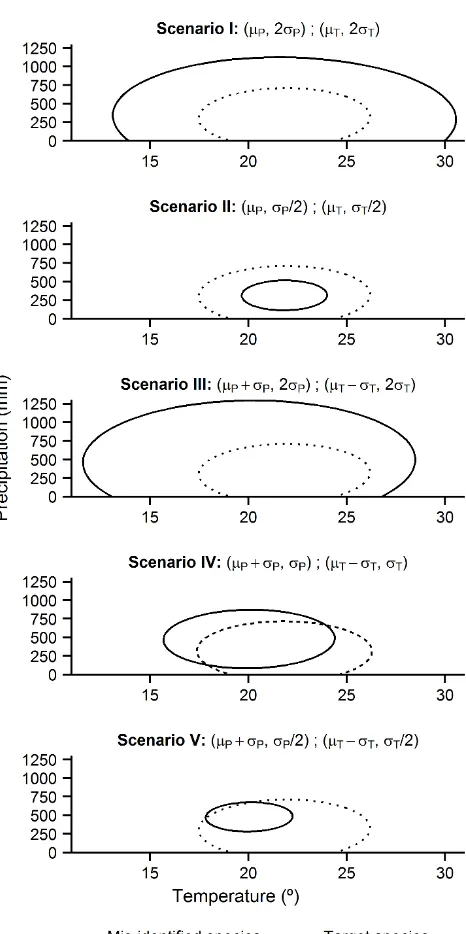
For the simulated contaminating species, the mean and standard deviation of P and T varied in standard deviation units in relation to the simulated target species defined above. Specifically, a specific contaminating species was simulated within five scenarios (scenarios I–V) as the impact of species misidentification would be expected to depend on the ecological difference between the species niches confused. Figure 2 shows the mean and standard deviation of P and T, and the resulting niche for the simulated target and contaminating species in all the scenarios. Specifically, the niche of the simulated contaminating species was defined relative to the simulated target species as being wider (scenarios I and III) and narrower (scenarios II and V). Both species have the same niche breadth in scenario IV. In addition, scenarios III, IV, and V define the simulated contaminating species with a shift in niche optimum, preferring cooler and wetter environmental conditions than the simulated target species. As a result of the scenarios defined, the niche of the simulated target and contaminating species were expected to diverge. The Bhattacharyya distance [39] was used to measure the divergence between the niches, which increased across the scenarios—the Bhattacharyya distance between the niche of the simulated target and contaminating species of scenarios I–V was 3.5 × 10⁻³, 9.4 × 10⁻³,
Figure 2. The ecological niche of the simulated target and contaminating species in five scenarios (ellipses show the 95% probability regions). The niche of the target species was defined as the multiplicative interaction of precipitation (P) and temperature (T). The response of the target species to P and T was defined using normal curves where the mean μ and standard deviation σ of P (μP, σP) and T (μT, σT) are 314.77 and 162.90, and 21.83
and 1.79, respectively. For the simulated contaminating species, μ and σ of P and T varied in standard deviation units in relation to the simulated target species as shown in each scenario (for example, the normal curve of P in scenario III used a mean value of μP + σP
and a standard deviation of 2σP).
species had a higher chance of being selected and, hence, the samples indicated ecological preferences of the species. In addition, the same strategy was used to create a testing sample for the purpose of estimating the prediction accuracy of the MaxEnt results while using simulated data. However, here there was the opportunity of generating data for absences as well as presences, allowing the calculation of standard accuracy measures such as the area under the receiver operating characteristic curve (AUC) [40]. A total of 1000 presences and 1000 absences were generated in the same manner outlined above, but using the inverse of environmental suitability (1 − Si) as weights for generating the
absences (i.e., locations with low environmental suitability for the species had a higher chance of being selected).
2.3. Modeling Procedures
MaxEnt (version 3.3.3k; [41]) was used in this study as it is one of the most popular methods to model species distributions. MaxEnt finds the species spatial distribution of maximum entropy (i.e., closest to uniform), subject to a set of constraints determined by the species data in use [11], which is equivalent to minimizing, in the environmental space, the relative entropy between the probability density estimated from the presence data and that one estimated from the landscape, or from a sample thereof, called background [42].
The default values of the MaxEnt’s parameters were used, except the feature types and output format. The term “feature” refers to an expanded set of transformations of the original environmental variables used, such as the product of all possible pair-wise combinations of variables [42]. Only the “hinge” feature type was used as it, alone, produces results similar to all the other feature types available in the software [43]. The ‘raw’ output format was used and interpreted as relative probability or a suitability index at a location for the presence of a species [44–46]. In addition, a “target-group” background was defined in the case of the real data to address sample bias. The target-group considered were the tree ferns detected in the island, including C. cooperi, C. medullaris, Cyathea sp., and D. antartica. The aim of a “target-group” background is to include spatial bias in the background as embedded in the presence-only data so that both become spatially biased in a similar manner. This procedure reduces the potential for the MaxEnt predictions to resemble the spatial bias included in the species data [43,47]. A total of 10,000 records (locations) were selected across the island through a weighted random sampling using as probability weights the inverse distance from the location to the closest tree fern presence identified in the field survey. In this way, locations closer to sampled locations were more likely to be selected and hence more represented in the background.
random records of the contaminating species. Thus, in the case of real data, the random records selected from the C. cooperi dataset were contaminated with records randomly selected from the C. medullaris dataset. However, here, the rate of 32% was not possible to investigate because each species record could be selected only one time per iteration to avoid duplicates, and at least 64 records of C. medullaris were needed while it has only 32 records. In the case of the simulated data, bootstrapping was applied in each scenario, meaning that the random records selected from the sample defined for the simulated target species were contaminated with records randomly selected from the sample of the simulated contaminating species defined in the relevant scenario.
Finally, predictions were produced for the contaminating species, which is equivalent to an error rate of 100%. In the case of the real data, a bootstrapping procedure was not applied here as the dataset of C. medullaris has only 32 records, which were used simultaneously to produce a model predicting the presence of C. medullaris across the island. In the case of the simulated data, predictions for the contaminating species defined in each scenario were calculated within a bootstrapping procedure similar to that described above, with bootstrap samples of size 200 randomly selected only from the sample of the contaminating species defined in the relevant scenario.
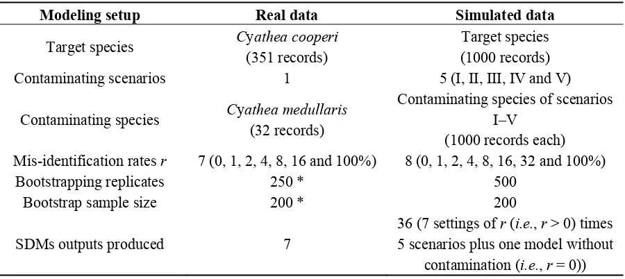
[image:9.595.76.526.518.719.2]Each bootstrapping procedure created 250 or 500 MaxEnt outputs, which needed to be summarized. Each location i in the island was assigned the mean value of the predictions calculated in the bootstrapping procedures for the real and simulated species. The mean of the predictions were kept for further analysis and are, hereafter, simply referred to as “predictions”. The 95% confidence intervals around the predictions were also calculated for each location. Additionally, the predictions were ranked in order of magnitude. Thus, the modeling results could be used in two different ways, based on either the value of the predictions or their relative rank order. These two distinct ways of representing SDM outputs are commonly considered in real-world applications [48,49]. Table 1 summarizes the modeling definitions applied.
Table 1. Summary of the modeling setup performed with MaxEnt.
Modeling setup Real data Simulated data
Target species Cyatheacooperi (351 records)
Target species (1000 records) Contaminating scenarios 1 5 (I, II, III, IV and V)
Contaminating species Cyatheamedullaris (32 records)
Contaminating species of scenarios I–V
(1000 records each) Mis-identification rates r 7 (0, 1, 2, 4, 8, 16 and 100%) 8 (0, 1, 2, 4, 8, 16, 32 and 100%)
Bootstrapping replicates 250 * 500 Bootstrap sample size 200 * 200
SDMs outputs produced 7
36 (7 settings of r (i.e., r > 0) times 5 scenarios plus one model without
contamination (i.e., r = 0))
* except when r = 100%, in which case only one replicate was run with a sample size of 32.
50 presences and 50 absences were randomly sampled 100 times from the testing sample to calculate 100 AUC values by means of the R package PresenceAbsence [50]. The mean of the 100 AUC values was calculated for each scenario and error rate and are hereafter referred to as “AUC values”.
2.4. Analyses
Two analyses (A and B) were performed to understand the nature of the effects of species misidentification on MaxEnt predictions. Another two analyses (C and D) were performed to assess the magnitude of the effects and their potential impacts of practical applications. The four analyses (Table 2) were performed for the results obtained with the real and simulated data.
Table 2. Summary of the analyses performed to examine the impacts of misidentification on the MaxEnt predictions.
Analysis Purpose Methods
A
Understanding whether species
misidentification caused a contraction or expansion of the predicted distribution of the target species.
Comparison of the estimate of the probability density function of the predictions produced with and without contaminated data. Estimates were obtained with the kernel method, namely the Gaussian smoothing kernel [51].
B
Identifying the direction of the contraction or expansion effects identified in Analysis A, namely whether the contaminating data shifted the MaxEnt predictions of the species presence towards the distribution of the contaminating species.
Calculation of Schoener’s D comparing the MaxEnt predictions produced using contaminated data (1%≤r≤32%) to both the predictions
produced using the gold standard data set (r = 0%) and the contaminating species (r = 100%).
C
Assessing the magnitude of the effects identified in the previous two analyses.
Number of pixels for which the MaxEnt
predictions produced using contaminated data and the gold standard data set differed significantly (i.e., the 95% confidence interval of the SDM predictions did not overlapped).
D
Assessing the potential impacts of species misidentification on practical applications that use SDM based analysis to identify priority areas such as in management.
Identification of the omission and commission errors committed using contaminated data while defining priority areas (i.e., the MaxEnt predictions that ranked in the top decile).
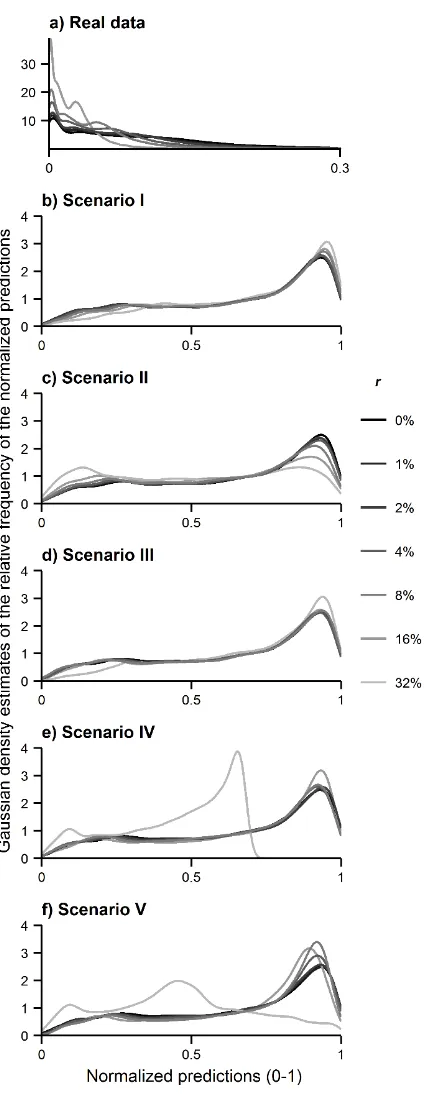
The relative frequency of the predicted values produced by MaxEnt across the island was examined in Analysis A. The comparison between the relative frequency of the predicted values produced with and without contaminated data allows for understanding of whether species misidentification caused a contraction or expansion of the predicted distribution of the target species. Specifically, when contraction occurs, the relative frequency of low prediction values is expected to increase at the expense of a decrease of the frequency of high prediction values; with expansion the opposite occurs. The Gaussian kernel density estimates of the prediction values were, thus, calculated by means of the R package ggplot2 [52]; kernel density estimates are close to histograms but facilitate legibility and interpretation.
produced using contaminated data (1%≤ r ≤32%) to both the predictions produced using the gold standard data set (r = 0%) and the contaminating species (r = 100%). The calculation of Schoener’s D is based on normalized prediction values (all predictions should sum to 1) and may be expressed as D = 1 − 1/2∑|pXi − pYi|, where pXi and pYi are the normalized prediction values on location i of the
SDM outputs being compared. Thus, Schoener’s D ranges between 0 and 1 and provides a measure of the similarity of two modeling outputs in the geographic space.
The MaxEnt outputs produced using contaminated data (1% ≤ r ≤ 32%) were, in Analysis C, compared again in the geographic space to the MaxEnt outputs produced using the gold standard data set (r = 0%). However, analysis C provides a measure of the magnitude of the effects identified in the previous analyses. The difference between the predictions obtained with and without contaminated data for a given location i was considered insignificant if the 95% confidence intervals of the predictions overlapped. The proportion of the locations of São Miguel whose predictions differed significantly was calculated.
Finally, the potential impacts of species misidentification on practical applications such as management were considered in Analysis D. Specifically, this analysis focused on only the locations that ranked in top decile (i.e., 10%), as an example, as sites with relatively higher prediction values are commonly targeted, such as for surveillance of early invasions of alien species. Such locations are hereafter referred to as priority areas. The omission and commission errors committed by MaxEnt in the definition of priority areas were calculated through the comparison of the location of the priority areas defined with and without contaminated data. Omission error is the proportion of the locations defined as priority areas using the gold standard data set but not when using contaminated data. Commission error is the proportion of the locations defined as priority areas using contaminated data but not when using the gold standard dataset.
3. Results
the predicted distribution of the target species expanded. Figure 3b,d shows that the relative frequency of high prediction values increased in scenario I and III as a function of the misidentification rate.
Figure 3. Gaussian kernel density estimates of the MaxEnt predictions: (a) real data; (b) simulated data in scenario I; (c) simulated data in scenario II; (d) simulated data in scenario III; (e) simulated data in scenario IV; and (f) simulated data in scenario V.
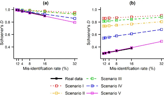
distribution of the target species was progressively shifted towards the distribution of the contaminating species as the misidentification rate increased. Specifically, Schoener’s D showed that the MaxEnt outputs became less similar to those produced using the gold standard data set, as expected, and became more similar to the outputs produced for the contaminating species. For example, as regards the tree ferns, Figure 4a shows that the similarity between the MaxEnt output obtained with r = 1% and that obtained with the gold standard data set (r = 0% ) is very high (Schoener’s D ∼1). As the value of r increased, the value of Schoener’s D decreased. That is, the distribution of C. cooperi predicted with increasing rates of error diverged progressively from the actual distribution of the species. On the contrary, in Figure 4b, the similarity between the MaxEnt output obtained using r = 1% and that obtained for the contaminating species (r = 100%) was very low (Schoener’s D ∼0.3), but increased with increasing values of r. This means that the use of misidentified records caused the predicted distribution of C. cooperi to become more similar to the distribution of the contaminating species C. medullaris. These trends observed in Figure 4 were in general consistent across the real data and the scenarios of the simulated data. The influence of the niche of the species was, in the context of Analysis B, irrelevant as the ecological distance between the niches of the target and contaminating species was expected to change merely the magnitude of the Schoener’s D values; in all cases Schoener’s D showed that the predicted distribution was shifted towards the distribution of the contaminating species, which meets the purpose of the analysis.
Figure 4. Similarity (Schoener’s D) between the MaxEnt outputs produced with and without contaminated data: (a) comparison between the contaminated outputs (1% ≤ r ≤ 32%) and those produced using the gold standard data set (r = 0%); and (b) comparison between the contaminated outputs (1% ≤ r ≤ 32%) and those produced using the contaminating species (r = 100%).
relatively higher prediction values in Figure 5b (r = 16%), highlighted by an arrow, correspond to the locations of higher prediction values for the contaminating species C. medullaris (Figure 5c). This means that the misidentified records shifted the predictions of presence of C. cooperi towards those of C. medullaris. Similar effects were visible in the results obtained with the simulated data. However, the simulated data also allowed assessment of scenarios in which the niche of the contaminating species was broader than that of the target species. In this situation the predicted distribution of the target species expanded (Figure 5d,e), particularly to zones at altitude in scenarios III–V because the distribution of the contaminating species was simulated to include such environments (Figure 2 and Figure 5f).
Figure 5. Some examples of predictions of presence of the real and simulated species produced by MaxEnt: (a) predictions of presence of C. cooperi produced using the gold standard data set (r = 0%); (b) predictions of presence of C. cooperi produced using contaminated data (r = 16%); (c) predictions of presence of the contaminating species C. medullaris (r = 100%); (d) predictions of presence of the simulated target species using the gold standard data set (r = 0%); (e) predictions of presence of the simulated target species using contaminated data in scenario III (r = 16%); and (f) predictions of presence of the simulated contaminating species in scenario III (r = 100%); Notes: greyscale from black (high prediction values) to white (low prediction values). Black arrows in parts (b) and (c) highlight an area where the influence of the distribution of the contaminating species over that of the target species is particularly noted when using contaminated data.
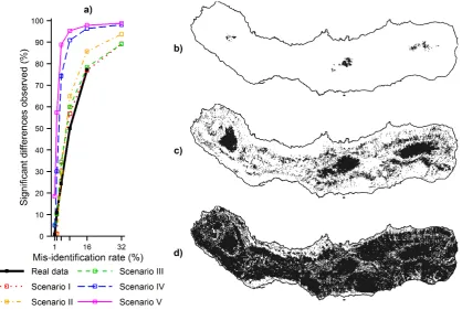
(Figure 6). However, the effects were very pronounced as a small increase of the misidentification rate caused a large proportion of predictions to differ significantly across São Miguel. For example, 1% of misidentified records used to model the distribution of C. cooperi changed significantly the MaxEnt predictions in only 1% of the locations of the island (Figure 6b); increasing r to 4 and 16% the proportion of significant differences increased to 24 and 77% of the locations respectively (Figure 6c,d). The results obtained with the simulated species were similar, and also allowed assessment of the influence of the niche of the contaminating species. The proportion of significant differences observed in the MaxEnt predictions increased from scenarios I–V (Figure 6a). That is, the proportion of predictions that differed significantly when using contaminated data increased, following the increasing ecological distance observed between the niches of the simulated target and contaminating species across scenarios I–V.
Figure 6. Magnitude of the effects caused by species mis-identification on the MaxEnt predictions: (a) proportion of the predictions that differed significantly at the various misidentification rates for the real and simulated species; (b) location of the predictions that changed significantly (in black) for C. cooperi using the misidentification rate of 1%; (c) Location of the predictions that changed significantly (in black) for C. cooperi using the misidentification rate of 4%; and (d) location of the predictions that changed significantly (in black) for C. cooperi using the misidentification rate 16%.
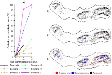
(omission errors), while locations of low relative probability of the species presence were erroneously included in the set of priority areas when contaminated data was used (commission errors). Furthermore, the results also showed that the size and location of the omission and commission errors depended on the distribution of the species confused. With regard to the simulated data, the size of the errors was positively related to the ecological distance between the niches of the target and contaminating species. Specifically, the errors increased from scenarios I–V (Figure 7a), which corresponds to an increasing ecological distance between the niches. The location of the errors was associated with the ecological preferences of the species. Omission errors tended to appear at locations preferred by the target species but not the contaminating species and commission errors tended to appear in opposite conditions. For example, Figure 7b–d show the location of the omission and commission errors committed while defining priority areas for C. cooperi with imperfect data. As the misidentification rate increased, the higher ranked predictions appeared progressively in the interior part of São Miguel, where C. medullaris occurs. These commission errors occurred at the expense of omission errors located elsewhere. Note that the real data used is a case in which the niche of the contaminating species is less widely distributed relative to that of the target species and, thus, the predicted distribution of C. cooperi contracted (Figure 3a). As a result, the location of the omission and commission errors reflects the contraction of a broader species distribution towards the narrow environments associated to the records of the contaminating species.
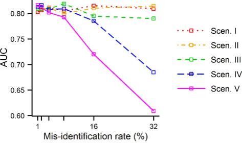
Finally, the impacts of misidentification error identified and measured in analyses A-D were less apparent in the AUC values calculated using the simulated data. Although the AUC values tended to decrease as the error rate, r, increased, as expected, the AUC values were constant until r was large. Only when the error rate was 16% in scenarios IV and V the AUC values clearly started to decrease (Figure 8).
Figure 8. AUC values of the MaxEnt outputs produced using the simulated data as a function of the misidentification error rate.
4. Discussion
Systematic misidentification of species and consequent production of contaminated spatial datasets impacts negatively on species distribution modeling. Species misidentification errors may act to change the predicted distribution of the target species while shifting the predicted distribution towards that of the contaminating species. The magnitude and direction of the changes is positively related to both the misidentification rate and the ecological difference between the distributions of the species confused.
Expansion of the predicted distribution of a species caused by misidentification errors have already been reported in the literature [31,32]. Here, however, it is evident that contraction can occur if the contaminating species is less widely dispersed than the target species. For example, Analysis A showed contraction effects in the MaxEnt results produced with real data (Figure 3a), in which the contaminating species was less widely distributed than the target species (Figure 1b). It is thus expected that systematic species misidentification error can often act to contract the predicted distribution of a target species since less-dispersed contaminating species may be rare and unfamiliar species and, hence, may be more prone to misidentification, more than well-known species.
used is free of error as in this study. Therefore, systematic species misidentification addressed in this paper could be a dangerous source of error in species distribution modeling as there may be no means available for its detection once a species dataset is used as if free of error.
Perhaps the main finding of this study is that the occurrence of misidentification errors in species data may compromise the goal behind the application of SDMs. For example, if the SDMs’ predictions are regarded as an estimate of probability [45], small rates of misidentification error may significantly change the prediction values produced, resulting in erroneous estimates of the probability of the species presence in much of the area in study. This was evident in the results for Analysis C above (Figure 6). Alternatively, the SDMs’ predictions may be regarded as ordinal, which is enough to identify areas with relatively higher probability of a species presence. In this case, SDMs are required to solve a simpler problem, which is to rank locations by order of probability of a species. The latter was the focus of Analysis D, which showed that systematic misidentification may also influence negatively the rank of the predictions and hence the identification of priority areas (Figure 7). Critically, misidentification errors may cause priority areas to include locations where the species is unlikely to actually occur, thus wasting efforts and resources, and overlooking locations where the species is likely to occur, thus possibly compromising the effectiveness of management actions.
The location of omission and commission errors committed while defining priority areas relate to the direction of the contraction or expansion effects outlined above. The latter was the focus of Analysis B, which showed that the predicted distribution of the target species was shifted towards the distribution of the contaminating species (Figure 4). As a result, areas incorrectly identified as priority areas (commission error) will tend to appear in locations close to environments ideal for the contaminating species. Locations that are worth of attention will tend, on the other hand, to be overlooked (omission error) across regions associated with environments preferred by the target species. This is evident, for example, in Figure 7d, which shows that the commission errors of the priority areas defined for C. cooperi appeared at altitude, in the interior of the island, where the contaminating species C. medullaris was detected (Figure 1b).
The four analyses performed with both real and simulated data show that the occurrence of systematic misidentification errors in species data is expected to degrade SDMs predictions in a wide variety of circumstances; the real dataset represented a common situation in which the species were not at equilibrium and the sample was spatially biased, while the simulated dataset represented a situation in which the species were at equilibrium and the sample unbiased.
Alternatively, outlier analysis may be used as a means for the detection and removal of suspicious records [57]. Outliers may, however, correspond to records of the species of interest. For example, outliers may correspond to individuals at the forefront of an invasion and thus provide important information that should be taken into account [58]. Note that records seen as outliers among records collected across regions of interest (e.g., an island) may be, after all, highly similar to records of the species collected across a larger region. Thus, it is important to take into considerations the entire range of environmental conditions known to be used by the species [59]. This is not sufficient, however, if a species is introduced into new regions where it meets no constraints [60], such as predation and competition, and thus has the opportunity of using new environments. Changing the modeling approach is also a possibility and thus occupancy models may be considered. This type of model allows for misidentification errors [24], but are demanding in data, such as several surveys over time, which may not be logistically possible or not applicable if biodiversity databases are used [8,10]. The present study, therefore, highlights that investment on quality should be a continuous concern with regard to data collection.
5. Conclusions
Despite the recent developments in methodologies for species distribution modeling, such as SDMs that use presence-only data and are able to compensate for sampling bias, the results call for careful identification of species. Systematic species misidentification errors were showed to impact negatively on species distribution modeling as they may act to change the predicted distribution of a species. Specifically, misidentification may act to contract or expand the predicted distribution towards that of the contaminating species. Species misidentification may, therefore, substantially change the output of SDMs. This problem may go largely unnoticed while assessing the accuracy of the predictions using common methods such as the AUC and thus influence negatively practical applications that use SDMs-based analyses. Therefore, the results presented re-emphasize the calls for an emphasis of data quality in SDMs studies such as those made by Lobo [61] and Cayuela, et al. [62]. In particular, this paper highlights that species misidentification should not be neglected in species distribution modeling. Acknowledgments
The authors thank Eduardo Brito de Azevedo for supplying the CIELO data. Hugo Costa was partly supported by a scholarship from InBIO-Research Network in Biodiversity and Evolutionary and supported by the PhD Studentship number SFRH/BD/77031/2011 from the “Fundação para a Ciência e Tecnologia” (FCT), funded by the “Programa Operacional Potencial Humano” (POPH) and the European Social Fund. Sílvia Jiménez was supported by an ERASMUS scholarship (254.6764356007004).
Author Contributions
Conflicts of Interest
The authors declare no conflict of interest. References
1. Guisan, A.; Thuiller, W. Predicting species distribution: Offering more than simple habitat models. Ecol. Lett. 2005, 8, 993–1009.
2. Elith, J.; Leathwick, J.R. Species distribution models: Ecological explanation and prediction across apace and time. Annu. Rev. Ecol. Evolut. Syst. 2009, 40, 677–697.
3. Guisan, A.; Zimmermann, N.E. Predictive habitat distribution models in ecology. Ecol. Model. 2000, 135, 147–186.
4. Barry, S.; Elith, J. Error and uncertainty in habitat models. J. Appl. Ecol. 2006, 43, 413–423. 5. Yañez-Arenas, C.; Guevara, R.; Martínez-Meyer, E.; Mandujano, S.; Lobo, J.M. Predicting
species’ abundances from occurrence data: Effects of sample size and bias. Ecol. Model. 2014, 294, 36–41.
6. Moudrý, V.; Šímová, P. Influence of positional accuracy, sample size and scale on modelling species distributions: A review. Int. J. Geogr. Inf. Sci. 2012, 26, 2083–2095.
7. Syfert, M.M.; Smith, M.J.; Coomes, D.A. The effects of sampling bias and model complexity on the predictive performance of maxent species distribution models. PLoS ONE 2013, 8, doi:10.1371/journal.pone.0055158.
8. Hortal, J.; Lobo, J.M.; Jiménez-Valverde, A. Limitations of biodiversity databases: Case study on seed-plant diversity in tenerife, canary islands. Conserv. Biol. 2007, 21, 853–863.
9. Guisan, A.; Graham, C.H.; Elith, J.; Huettmann, F.; The NCEAS Species Distribution Modelling Group. Sensitivity of predictive species distribution models to change in grain size. Divers. Distrib. 2007, 13, 332–340.
10. Graham, C.H.; Ferrier, S.; Huettman, F.; Moritz, C.; Peterson, A.T. New developments in museum-based informatics and applications in biodiversity analysis. Trend. Ecol. Evol. 2004, 19, 497–503.
11. Phillips, S.J.; Anderson, R.P.; Schapire, R.E. Maximum entropy modeling of species geographic distributions. Ecol. Model. 2006, 190, 231–259.
12. Hanberry, B.B.; He, H.S.; Dey, D.C. Sample sizes and model comparison metrics for species distribution models. Ecol. Model. 2012, 227, 29–33.
13. Hefley, T.J.; Baasch, D.M.; Tyre, A.J.; Blankenship, E.E. Correction of location errors for presence-only species distribution models. Method. Ecol. Evolut. 2014, 5, 207–214.
14. Kramer-Schadt, S.; Niedballa, J.; Pilgrim, J.D.; Schröder, B.; Lindenborn, J.; Reinfelder, V.; Stillfried, M.; Heckmann, I.; Scharf, A.K.; Augeri, D.M.; et al. The importance of correcting for sampling bias in maxent species distribution models. Divers. Distrib. 2013, 19, 1366–1379.
16. Varela, S.; Anderson, R.P.; García-Valdés, R.; Fernández-González, F. Environmental filters reduce the effects of sampling bias and improve predictions of ecological niche models. Ecography 2014, 37, 1084–1091.
17. Dormann, C.F.; McPherson, J.M.; Araújo, M.B.; Bivand, R.; Bolliger, J.; Carl, G.; Davies, R.G.; Hirzel, A.; Jetz, W.; Kissling, W.D.; et al. Methods to account for spatial autocorrelation in the analysis of species distributional data: A review. Ecography 2007, 30, 609–628.
18. Santika, T.; Hutchinson, M.F. The effect of species response form on species distribution model prediction and inference. Ecol. Model. 2009, 220, 2365–2379.
19. Václavík, T.; Kupfer, J.A.; Meentemeyer, R.K. Accounting for multi-scale spatial autocorrelation improves performance of invasive species distribution modelling (iSDM). J. Biogeogr. 2012, 39, 42–55.
20. de Oliveira, G.; Rangel, T.F.; Lima-Ribeiro, M.S.; Terribile, L.C.; Diniz-Filho, J.A.F. Evaluating, partitioning, and mapping the spatial autocorrelation component in ecological niche modeling: A new approach based on environmentally equidistant records. Ecography 2014, 37, 637–647. 21. Meyer, C.B.; Thuiller, W. Accuracy of resource selection functions across spatial scales. Divers.
Distrib. 2006, 12, 288–297.
22. Fernandes, R.; Vicente, J.; Georges, D.; Alves, P.; Thuiller, W.; Honrado, J. A novel downscaling approach to predict plant invasions and improve local conservation actions. Biol. Invasion. 2014, 16, 2577–2590.
23. Alldredge, M.W.; Pacifici, K.; Simons, T.R.; Pollock, K.H. A novel field evaluation of the effectiveness of distance and independent observer sampling to estimate aural avian detection probabilities. J. Appl. Ecol. 2008, 45, 1349–1356.
24. Bailey, L.L.; MacKenzie, D.I.; Nichols, J.D. Advances and applications of occupancy models. Method. Ecol. Evolut. 2013, 5, 1269–1279.
25. Archaux, F.; Gosselin, F.; Bergès, L.; Chevalier, R. Effects of sampling time, species richness and observer on the exhaustiveness of plant censuses. J. Veg. Sci. 2006, 17, 299–306.
26. Tillett, B.J.; Field, I.C.; Bradshaw, C.J.A.; Johnson, G.; Buckworth, R.C.; Meekan, M.G.; Ovenden, J.R. Accuracy of species identification by fisheries observers in a north Australian shark fishery. Fish. Res. 2012, 127–128, 109–115.
27. Hull, J.M.; Fish, A.M.; Keane, J.J.; Mori, S.R.; Sacks, B.N.; Hull, A.C. Estimation of species identification error: Implications for raptor migration counts and trend estimation. The J. Wildl. Manag. 2010, 74, 1326–1334.
28. Shea, C.P.; Peterson, J.T.; Wisniewski, J.M.; Johnson, N.A. Misidentification of freshwater mussel species (Bivalvia: Unionidae): Contributing factors, management implications, and potential solutions. J. North. Am. Benthol. Soc. 2011, 30, 446–458.
29. Meier, R.; Dikow, T. Significance of specimen databases from taxonomic revisions for estimating and mapping the global species diversity of invertebrates and repatriating reliable specimen data. Conserv. Biol. 2004, 18, 478–488.
30. Scott, W.A.; Hallam, C. Assessing species misidentification rates through quality assurance of vegetation monitoring. Plant Ecol. 2003, 165, 101–115.
32. Molinari-Jobin, A.; Kéry, M.; Marboutin, E.; Molinari, P.; Koren, I.; Fuxjäger, C.; Breitenmoser-Würsten, C.; Wölfl, S.; Fasel, M.; Kos, I.; et al. Monitoring in the presence of species misidentification: The case of the Eurasian lynx in the Alps. Anim. Conserv. 2012, 15, 266–273.
33. Beerkircher, L.; Arocha, F.; Barse, A.; Prince, E.; Restrepo, V.; Serafy, J.; Shivji, M. Effects of species misidentification on population assessment of overfished white marlin tetrapturus albidus and roundscale spearfish T. georgii. Endanger. Species Res. 2009, 9, 81–90.
34. Silva, L.; Ojeda-Land, E.; Rodríguez-Luengo, J.L. Invasive Terrestrial Flora and Fauna of Macaronesia. Top 100 in Azores, Madeira and Canaries; ARENA: Ponta Delgada, Portugal, 2008. 35. Borges, P.A.V.; Amorim, I.R.; Cunha, R.; Gabriel, R.; Martins, A.F.; Silva, L.; Costa, A.;
Vieira, V. Azores. In Encyclopedia of Islands; Gillespie, R.G., Clague, D.A., Eds.; University of California Press: Oakland, CA, USA, 2009; pp. 70–75.
36. Robinson, R.C.; Sheffield, E.; Sharpe, J.M. Problem ferns: Their impact and management. In Fern Ecology; Mehltreter, K., Walker, L.R., Sharpe, J.M., Eds.; Cambridge University Press: Cambridge, UK, 2010; pp. 255–322.
37. Azevedo, E.B.; Pereira, L.S.; Itier, B. Modelling the local climate in island environments: Water balance applications. Agric. Water Manag. 1999, 40, 393–403.
38. Projectos Climaat e Climarcost. Available online: www.climaat.angra.uac.pt (accessed on 10 November 2015).
39. Theodoridis, S.; Koutroumbas, K. Pattern Recognition, 4th ed.; Academic Press: Burlington, MA, USA, 2009.
40. Fielding, A.H.; Bell, J.F. A review of methods for the assessment of prediction errors in conservation presence/absence models. Environ. Conserv. 1997, 24, 38–49.
41. Maxent Software for Species Habitat Modeling. Available online: http://www.cs.princeton.edu/ ~schapire/maxent (accessed on 10 November 2015).
42. Elith, J.; Phillips, S.J.; Hastie, T.; Dudík, M.; Chee, Y.E.; Yates, C.J. A statistical explanation of maxent for ecologists. Divers. Distrib. 2011, 17, 43–57.
43. Phillips, S.J.; Dudík, M. Modeling of species distributions with Maxent: New extensions and a comprehensive evaluation. Ecography 2008, 31, 161–175.
44. Royle, J.A.; Chandler, R.B.; Yackulic, C.; Nichols, J.D. Likelihood analysis of species occurrence probability from presence-only data for modelling species distributions. Method. Ecol. Evolut. 2012, 3, 545–554.
45. Phillips, S.J.; Elith, J. On estimating probability of presence from use-availability or presence-background data. Ecology 2013, 94, 1409–1419.
46. Yackulic, C.B.; Chandler, R.; Zipkin, E.F.; Royle, J.A.; Nichols, J.D.; Campbell Grant, E.H.; Veran, S. Presence-only modelling using Maxent: When can we trust the inferences? Method. Ecol. Evolut. 2013, 4, 236–243.
47. Merow, C.; Smith, M.J.; Silander, J.A. A practical guide to Maxent for modeling species’ distributions: What it does, and why inputs and settings matter. Ecography 2013, 36, 1058–1069. 48. Strubbe, D.; Matthysen, E. Predicting the potential distribution of invasive ring-necked parakeets
49. Costa, H.; Aranda, S.C.; Lourenço, P.; Medeiros, V.; de Azevedo, E.B.; Silva, L. Predicting successful replacement of forest invaders by native species using species distribution models: The case of Pittosporum undulatum and Morella faya in the Azores. For. Ecol. Manag. 2012, 279, 90–96.
50. Freeman, E.A.; Moisen, G. PresenceAbsence: An R package for presence absence analysis. J. Stat. Softw. 2008, 23, 1–31.
51. Silverman, B.W. Density Estimation for Statistics and Data Analysis; Chapman and Hall: London, UK, 1986; Volume 26.
52. Wickham, H. ggplot2: Elegant Graphics for Data Analysis; Springer: New York, NY, USA, 2009; p. 212.
53. Schoener, T.W. The Anolis lizards of Bimini: Resource partitioning in a complex fauna. Ecology 1968, 49, 704–726.
54. Warren, D.L.; Glor, R.E.; Turelli, M.; Funk, D. Environmental niche equivalency versus conservatism: Quantitative approaches to niche evolution. Evolution 2008, 62, 2868–2883.
55. Crall, A.; Newman, G.; Jarnevich, C.; Stohlgren, T.; Waller, D.; Graham, J. Improving and integrating data on invasive species collected by citizen scientists. Biol. Invasion. 2010, 12, 3419–3428.
56. Fitzpatrick, M.C.; Preisser, E.L.; Ellison, A.M.; Elkinton, J.S. Observer bias and the detection of low-density populations. Ecol. Appl. 2009, 19, 1673–1679.
57. Soley-Guardia, M.; Radosavljevic, A.; Rivera, J.L.; Anderson, R.P. The effect of spatially marginal localities in modelling species niches and distributions. J. Biogeogr. 2014, 41, 1390–1401.
58. Václavík, T.; Meentemeyer, R.K. Equilibrium or not? Modelling potential distribution of invasive species in different stages of invasion. Divers. Distrib. 2012, 18, 73–83.
59. Broennimann, O.; Guisan, A. Predicting current and future biological invasions: Both native and invaded ranges matter. Biol. Lett. 2008, 4, 585–589.
60. Jiménez-Valverde, A.; Peterson, A.T.; Soberón, J.; Overton, J.M.; Aragón, P.; Lobo, J.M. Use of niche models in invasive species risk assessments. Biol. Invasion. 2011, 13, 2785–2797.
61. Lobo, J.M. More complex distribution models or more representative data? Biodivers. Inform. 2008, 5, 14–19.
62. Cayuela, L.; Golicher, D.J.; Newton, A.C.; Kolb, M.; de Alburquerque, F.S.; Arets, E.J.M.M.; Alkemade, J.R.M.; Pérez, A.M. Species distribution modeling in the tropics: Problems, potentialities, and the role of biological data for effective species conservation. Trop. Conserv. Sci. 2009, 2, 319–352.