Railway bridge asset management using a Petri Net modelling approach

Railway bridge asset management using a Petri-Net modelling approach

P. C. Yianni & D. Rama & L. C. Neves & J. D. Andrews

Centre for Risk and Reliability Engineering, University of Nottingham, Nottingham, UK

ABSTRACT: Infrastructure assets can be difficult to manage due to the array of defects, the variety of

en-vironmental situations and the different operational scenarios. A number of studies have tried to model bridge asset management. The main focus of these models has been on the deterioration profiling as capturing this can be complex. The model presented tries to model railway bridge detrioration as well as the inspection and intervention processes to give a more rounded overview of railway bridge asset management. A Petri-Net (PN) modelling approach is used accompanied by historical data, used to calibrate the deterioration of the model. Industry policies are used to govern the inspection and intervention procedures. Various aspects of the model have been adjusted or enhanced by industry experts. The model is simulated to provide essential outputs for railway bridge portfolio mangers.

1 INTRODUCTION

The railway network is critical to the UK economic output. Both commuters and freight rely heavily on the network. The pressure on the railway network to increase its throughput is high. A vast increase in throughput is predicted with the introduction of mov-ing block signallmov-ing; this means that trains can run closer together with tighter schedules. Coupled with increasingly more powerful tractive units, the stresses on the network will be tremendous. Therefore, more effective management of the assets is required to be able to cope with the increased demand. The focus of this study is civil structures; in particular railway bridges.

One of the first challenges for a railway operator is to understand how their portfolio of bridges be-haves. Construction of a modern bridge is governed by legislation (Eurocode 1996) which recommends a 100 year design life. However there is little guid-ance on how to manage the structure over those 100 years. This is made more complex by the fact that bridges degrade by different means, are subjected to different conditions both operationally and environ-mentally and finally, have been managed in different ways over their lifetime. Therefore management of a portfolio of bridges is a complex and demanding chal-lenge.

2 STOCHASTIC MODELS

2.1 Markov Based Models

Bridge asset management has had a number of stud-ies involving stochastic techniques, most notably, Markov based models. Frangopol, Kallen, & van Noortwijk 2004 state that structural deterioration is inherently stochastic by nature and therefore a stochastic modelling approach is most appropriate. Similarly, Morcous, Lounis, & Cho 2010 state that structural deterioration is a complex process which involves much uncertainty in the “micro-response” of the structure. Therefore a stochastic model offers a more robust approach that will more closely mimic the real-world process.

Offi-cials (AASHTO) to create Pontis, one of the most widespread Bridge Management Systems (BMSs). Pontis has been used in over 45 US states to manage in excess of 500,000 bridges (Sobanjo & Thompson 2011).

Another study which used a Markov approach was Scherer & Glagola 1994. The study took place in Vir-ginia, USA with 13,000 bridges. This study used 7 condition states with 1 representing a potentially haz-ardous state, to 7 representing an “as new” state. The authors state that a Markov chain approach would create too many states to model with contemporary computing facilities. The authors begin an exercise to group bridges by key characteristics based on the: bridge age, number of spans, bridge type, traffic load-ing and climate. In total the authors manage to col-late the 13,000 bridges into 216 characteristic groups. The study demonstrated an approach to overcoming the state expansion problem with Markov based mod-els. However, the authors do recognise that in some instances, bridges that were initially in one group may qualify for another group at a later date if there are op-erational or network changes.

Markov models are used as the back-end of many of the BMSs used globally. They have had unparal-leled adoption in the field of bridge asset manage-ment. Their suitability extends to many other fields including highways, water distribution and sewerage works (Morcous 2006). However, as with any tech-nique, there are limitations. Some of the limitations are Markovian limitations and some are limitations to using the Markov approach for bridge asset manage-ment. Firstly, Markov based models are usually cal-ibrated with data, however there are often borderline candidates that require expert judgement to categorise properly. Frangopol, Kallen, & van Noortwijk 2004 makes the case that a more detailed measurement cri-teria, possibly continuous in nature, would be supe-rior. Secondly, on the subject of calibration, calculat-ing the TPMs can be difficult and often requires ad-justment using expert judgement (Frangopol, Kallen, & van Noortwijk 2004). Thirdly, many studies disre-gard inspection data when the condition has improved as it is difficult to be certain which elements were re-paired (Robelin & Madanat 2007, Morcous, Rivard, & Hanna 2002). Lastly, a Markovian limitation is the state expansion problem. This is where the number

of model states follows Sn _{where S is the number}

of condition states andn is the number of bridges in

the study (British Standards Institution 2012). Scherer & Glagola 1994 tried to overcome this limitation by grouping bridges, however other limitations were in-troduced.

2.2 Petri-Net Based Models

PNs (Petri 1962) are not as common as other stochas-tic techniques, but have been gaining momentum in infrastructure modelling, manufacturing and

eco-nomics (British Standards Institution 2012). PNs have been used extensively in this study and are described in more detail in Section 3. Recent work by (Andrews 2013) suggests that PNs are suitable for infrastructure modelling as they have an inherent flexibility whilst maintaining the stochastic nature desired in bridge asset management modelling. The approach used 4 condition states to model deterioration ranging from a new condition to a condition requiring line speed restrictions. The model was designed for track asset management, however many of the techniques shown are transferable.

Another study performed by Rama & Andrews 2013 split the model into smaller modules known as “Sub-Nets” which usually perform a specific func-tion e.g. an inspecfunc-tion Sub-Net. A number of differ-ent Sub-Nets were developed to model compondiffer-ent de-terioration, inspection and intervention. A modelling hierarchy was presented in which the Sub-Nets were linked to interact with one another. An interesting ad-dition was the inclusion of a resource allocation Sub-Net. This was created to simulate if a maintenance team was occupied or not. The authors mention that having a library of different Sub-Nets would make it easier to create a modular modelling system where the relevant Sub-Nets were linked together to create a detailed model of the real-world system.

Bridge asset management models have been cre-ated using PNs (Le & Andrews 2014a, Le & An-drews 2014b). The study focused on metallic bridges. A number of Sub-Nets were created to model the dif-ferent processes. Again, 4 condition states were se-lected, however rather than describe the condition of the element, they were aligned with the intervention that would be required to repair the element i.e. rather than being in a “good” state, the state was marked “requires minor intervention”. This system makes the condition more clear from a management perspective (Yang, Pam, & Kumaraswamy 2009). The model in-cludes both the condition of the metallic element and the element coating, a vital factor in the corrosion of metallic elements. The authors run simulations on the model; the simulated period was 60 years which took 10 minutes to simulate with convergence reached af-ter 200 simulations.

The models which have been described show the application of PNs in infrastructure asset manage-ment modelling. They provide a convincing argu-ment that PNs are suitable for this type of modelling and that they are useful for bridge asset management modelling. Considering the flexibility required in the model and the numerous Markov limitations (see Sec-tion 2.1) it may be preferable to use PNs for bridge asset management modelling.

3 PETRI-NETS

and transitions, which connect the places. Tokens oc-cupy places and are representative of bridge elements in this study. I.e. an element, represented by a to-ken, could occupy the place marked “poor condition” which would indicate the condition of the element. Transitions move the token from place to place, in-dicating a movement in the element condition; this could be used to represent deterioration, for instance. Arcs are used to graphically show the dependencies between places and transitions. No two places or tran-sitions can be joined directly with an arc. The compo-nents of a PN can be seen in Figure 1. More details about PNs can be found in Reisig 2013.

Place Place with token Arc Transition

Figure 1: Components of a Petri-Net

3.1 Coloured Petri-Nets

Coloured Petri-Nets (CPNs), developed by Jensen 1997 are an extension to PNs. They allow a num-ber of sophisticated features to be built into PNs. Firstly, each of tokens holds the ability to contain data within them, known as tuple information. This is useful for identifying individual elements and track-ing them through the model. The fact that tokens are now distinguishable means that transitions act differ-ently upon them. This has the benefit of the models being more compact as when more elements are to be modelled it is simply a case of adding in the ap-propriate number of tokens (British Standards Insti-tution 2004). The second feature that CPNs enable is advanced transition functions. Rather than the basic rules which apply to transitions in PNs, CPNs allow customised transitions. This allows PNs to be married to programming code to make advanced transitions that perform sophisticated decisions. In the case of bridge management, this allows some of the processes to be mimicked more closely and more elegantly than with simple PNs.

4 DETERIORATION, INSPECTION AND

MAINTENANCE POLICIES

4.1 Condition States

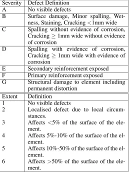
Network Rail (NR) identify different defects for dif-ferent material types. Each of the defects has a gra-dated scale according to their extent. This system is known as the Severity Extent Rating (SevEx). The SevEx state is used to identify the defect and the ex-tent of the defect, but varies according to material type. Materials that suffer from a wider array of de-fects have more SevEx states overall. For example, with concrete structures, the exemplar material type selected for this study, the 31 SevEx ratings range

from A1, the new condition, to G6, permanent struc-tural deformation. When looking at historical data, it is clear that the most common defects for concrete are cracking and spalling. Nielsen, Raman, & Chattopad-hyay 2013 found that cracking and spalling is the ma-jor driver in 89.9% of all concrete defects. The defect definitions and extents for concrete structures can be seen in Table 1.

Table 1: SevEx defect definitions and extents for concrete struc-tures (Network Rail 2012)

Severity Defect Definition

A No visible defects

B Surface damage, Minor spalling,

Wet-ness, Staining, Cracking<1mm wide

C Spalling without evidence of corrosion,

Cracking≥1mm wide without evidence

of corrosion

D Spalling with evidence of corrosion,

Cracking≥1mm wide with evidence of

corrosion

E Secondary reinforcement exposed

F Primary reinforcement exposed

G Structural damage to element including

permanent distortion

Extent Definition

1 No visible defects

2 Localised defect due to local

circum-stances.

3 Affects <5% of the surface of the

ele-ment.

4 Affects 5%-10% of the surface of the

el-ement.

5 Affects 10%-50% of the surface of the

el-ement.

6 Affects >50% of the surface of the

ele-ment.

4.2 Inspection Interval

NR policies describe two types of inspection. During a detailed inspection, each element of the structure is sketched and annotated with the defects. Then the ap-propriate SevEx condition is applied to each element and recorded. In accordance with the NR policies, de-tailed inspections are completed within touching dis-tance. Visual inspections are carried out on an annual basis and are much less rigorous. They involve us-ing the previous detailed inspection results and scan-ning the elements for any signs of significant condi-tion change. No scoring is carried out during visual inspections. They are used to avoid risk of sudden fail-ure as oppose to tracking long term corrosion. Refer-ences to inspections in this work are referring to the detailed inspections.

a risk score from which the appropriate inspection in-terval can be found. Rather than have to convert from SevEx to the risk score to find the time interval, a back conversion was performed to be able to trans-late the SevEx condition directly to the inspection in-terval. This allows the inspection intervals to be built straight into the model allowing for dynamic selection during simulation.

Broadly, the policy suggests that elements which are in better condition require less monitoring. Those which are in poorer condition require closer monitor-ing. The policies state different inspection intervals for different materials. For concrete elements, the in-tervals are 12 years for elements in good condition, 6 years for elements in moderate condition and 3 years for elements in poor condition.

4.3 Maintenance Actions

NR perform inspections on the elements of their as-sets and produce a SevEx score for each of them. The SevEx score is then converted to an index known as the Bridge Condition Marking Index (BCMI). The BCMI is then used to check the appropriate mainte-nance action. Each material type is assigned a “Ba-sic Safety Limit” which is a BCMI score that can-not be breached. Beyond the “Basic Safety Limit” the element would have to be replaced urgently. Overall there are three types of maintenance action: Minor Repair, Major Repair and Replacement. The threshold for Minor Repair starts where A1, the “as new” con-dition ends. The threshold for Major Repair is depen-dant on the material type. The Replacement thresh-old is set at the “Basic Safety Limit” of the particu-lar material type. The limits are quite strict which of-ten means that any defects are quickly dealt with and not left to develop further. The thresholds were back converted from BCMI to SevEx so that they could be directly incorporated into the model. This means that decisions on maintenance actions can be dynami-cally simulated in the model. The SevEx element con-ditions and their related maintenance actions can be seen in Table 2.

Table 2: Table showing the SevEx state thresholds for different maintenance actions.

Maintenance Action

States

Minor Repair B2-B4, C2-C3, D2

Major Repair B5-B6, C4-C6, D3-D5, E2-E4, F2-F3 Replacement D6, E5-E6, F4-F6, G2-G6

5 DATA SOURCE

A number of datasets were used for this study. The Structure Condition Marking Index (SCMI) database contains the records of element condition in both SevEx and BCMI; this can be used to track dete-rioration over time. The Cost Analysis Framework

(CAF) and MONITOR databases contain data re-garding interventions; CAF is used for larger work items where exterior contractors were used. MONI-TOR is for smaller work items that the NR mainte-nance teams carry out. Finally, the Civil Asset Reg-ister and Reporting System (CARRS) contains the structure identification information used to marry up the information between the datasets.

The total number of bridges on which inspections were carried out is 25,949. Each bridge is split up into a hierarchy of: Major elements, Minor elements and Sub-Minor Elements. The total number of inspected Major elements is 273,427. Each of those is split up into Minor elements. The total number of inspected Minor elements is 563,150. Finally, the total number of inspections on Sub-Minor elements was 1,397,748. This study uses concrete main girders as the exem-plar element. This is because concrete bridges are be-coming increasingly more popular and therefore their management will be progressively more important. Additionally, main girders are the main structural sup-port of the deck and therefore one of the most critical elements. The total number of concrete bridges in the databases is 4,434. At least two inspections on the el-ements are required to ascertain the rate of change of

condition. The number of repeat (x≥2) inspections on

concrete main girders totals 407,708.

6 PETRI-NET MODEL

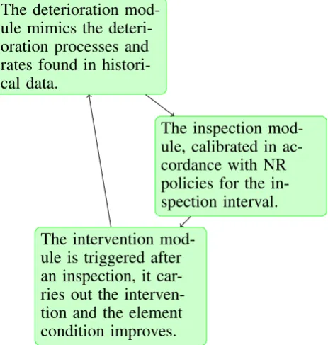
The modelling approach taken in this study is a bottom-up approach. To that effect, the model is on an asset and sub-asset level rather than a network level. The model itself represents a bridge asset with the to-kens in the model representing the elements of the bridge. To model a complete asset, the appropriate number of tokens needs to added corresponding to the number of elements wished to be modelled. In-teractions are carried out between the parent/child el-ements i.e. the condition of a Minor element depends on the condition of the Sub-Minor elements that it is comprised of. Interactions between parent/parent or child/child elements are not considered in this study, however the capability is present in the model. The model is organised into modules. Each of the modules mimics a different process; different techniques and data fitting procedures are used. The main modules that build the framework of the PN bridge model are the deterioration, inspection and intervention mod-ules. An overview of their interactions can be seen in Figure 2.

6.1 Deterioration

6.1.1 Calibrating Deterioration

Fail-The deterioration mod-ule mimics the deteri-oration processes and rates found in histori-cal data.

The inspection mod-ule, calibrated in ac-cordance with NR policies for the in-spection interval.

The intervention mod-ule is triggered after an inspection, it car-ries out the interven-tion and the element condition improves.

Figure 2: The overall framework of the PN model. The modules for deterioration, inspection and intervention are shown and how they interact.

ures (MTTFs). Failure in this instance refers to the movement from the initial condition to the destination condition. The MTTF was calculated with the follow-ing equation:

M T T FB2→B3=

t·nB2

mB2→B3

(1)

where mB2→B3 is the occurrences of elements that

move from conditionB2to conditionB3;nB2 is the

number of elements that occupy conditionB2 at the

beginning of the time interval andt is the time

inter-val. The failure rate can be calculated as follows:

λB2→B3 =

1

M T T FB2→B3

(2)

where λB2→B3 is the failure rate between condition

B2to conditionB3. In the PN model, each of the

de-terioration transitions are embedded with their corre-sponding failure rate. I.e. the transition which moves

the token(s) from conditionB2to condition B3will

be embedded withλB2→B3 so that the same

deterio-ration profile found from historical data can be repli-cated in the model. Each of these transitions is em-bedded with a different failure rate depending on the places they interact with. Table 3 shows some exam-ples of the MTTFs and failure rates between condition states.

6.1.2 Deterioration Module

The deterioration module captures the profile of the element deterioration over time. The SevEx states, used by NR for condition monitoring, are used di-rectly in the module to model deterioration. The ad-vantages of using this system include: 1) allowing ef-fective transformation from the SCMI database 2) ex-act defect definitions provided by the SevEx policy

Table 3: Example MTTFs calculated from historical data. Each transition in the deterioration module will be embedded with its corresponding failure rate depending on the places it connects.

State From, To

Number of Occur-rences

MTTF (years) Failure rate (years,10−2₎

A1,B2 2335 292.2835 0.3421 A1,B3 23550 28.9801 3.4506 A1,C2 317 2152.9400 0.0464 B2,B3 1103 50.6817 1.9731 B2,C2 62 901.6451 0.1109 B2,C3 706 79.1813 1.2629 B3,B4 5046 62.0154 1.6125 B3,C3 3627 86.2779 1.1590 B3,C4 1437 217.7661 0.4592

documents 3) avoiding conversion which has inherent losses associated with it and finally 4) the results of the simulation can be directly compared to the system already used by NR.

The module can be seen in Figure 3. The places, represented by the round nodes, are marked with the SevEx state that they represent. The transitions, rep-resented by the grey squares, connect the places. For

instance, transition T1 connects places A1 and B2.

This transition would be embedded with the failure rate corresponding to the historical movement of

el-ements fromA1to B2. As elements deteriorate over

time, this is mimicked in the model by tokens, rep-resenting elements, moving from place to place gov-erned by the failure rates embedded in the transitions.

This can be seen in the figure in places B2 and B3

as these are marked with tokens. This represents two Sub-Minor elements which are at different stages of deterioration. One of the advantages of CPNs is that tokens can be added to the module to represent as many elements as required.

A1

B2 B3

C2 C3

Pending Condition

Condition Determined Condition Change

T1 T2

T3

T4

T5 T6 T7

T8

T10 T9

A1

B2 B3

C2 C3

Minor Repairs

Major Repairs

Minor Repair Required

Major Repair Required

Replacement Required Intervention Planned

Between Inspection

During Inspection

Inspection Occurred

T13 T14 T15 T16

T11

T12

Between Intervention

Intervention Commences

T17 T18

Petri-Net for a Minor Element: Main External Girder (MGE), Concrete (C). All advanced transitions functions are represented with dashed arcs. WhereD/Prepresents a decision making probability transition that uses a ran-dom number to determine which probability the token is placed into e.g. (10%,80%,10%) if one of the inputs is designed to inhibit then the other options increase pro-portionately i.e. if the first 10% was inhibited then the options would become 80%+(80/90*10) = 88.89% and 10%+(10/90*10) = 11.11%;D/Mrepresents a transi-tion functransi-tion where a decision is based on marking, for instance it may determine the worst condition from the Sub-Minor Element conditions and places a token in the relevant place;Rrepresents a transition that is designed to reset a place or multiple places.

Transition Delay Type D/M D/P R T1 Stochastic No No No T2 Stochastic No No No T3 Stochastic No No No T4 Stochastic No No No T5 Stochastic No No No T6 Stochastic No No No T7 Stochastic No No No T8 Stochastic No No No T9 Instant No No Yes T10 Instant Yes No Yes T11 Conditional Yes No No T12 Small Delay (ε) No No Yes T13 Instant Yes Yes No T14 Instant Yes Yes No T15 Instant Yes Yes No T16 Instant Yes Yes No T17 Conditional Yes No Yes T18 Conditional Yes Yes Yes

Figure 3: The PN deterioration module. States A1 to C3 are shown for clarity. For concrete elements the states, A1 to G6, total 31 states.

6.2 Inspection Module

(Net-work Rail 2010c). The condition of the elements, pro-cessed in the deterioration module, is a factor which the inspection module assesses. The NR policies have different inspection intervals depending on the condi-tion of the element. The same guidelines are built into the inspection module, which can be seen in Figure 4.

The inspection module starts with transition T11,

which has dashed input arcs. These represent the deci-sion making capability of the transition. It assesses the places to determine what condition the element is in from which the appropriate inspection interval can be selected. Once that time has passed, the transition ab-sorbs the token from the “Between Inspection” state and outputs a token in the “During Inspection” state to show that the inspection process has begun. Once

the inspection has been completed, transitionT12

re-verts the module state back to “Between Inspection” where the module waits for the next inspection. A1 B2 B3 C2 C3 Pending Condition Condition Determined Condition Change

T1 T2

T3

T4

T5 T6 T7

T8 T10 T9 A1 B2 B3 C2 C3 Minor Repairs Major Repairs

Minor Repair Required

Major Repair Required

Replacement Required Intervention Planned

Between Inspection

During Inspection

Inspection Occurred

T13 T14 T15 T16

T11 T12 Between Intervention Intervention Commences T17 T18

Petri-Net for a Minor Element: Main External Girder (MGE), Concrete (C). All advanced transitions functions are represented with dashed arcs. WhereD/P represents a decision making probability transition that uses a ran-dom number to determine which probability the token is placed into e.g. (10%,80%,10%) if one of the inputs is designed to inhibit then the other options increase pro-portionately i.e. if the first 10% was inhibited then the options would become 80%+(80/90*10) = 88.89% and 10%+(10/90*10) = 11.11%;D/Mrepresents a transi-tion functransi-tion where a decision is based on marking, for instance it may determine the worst condition from the Sub-Minor Element conditions and places a token in the relevant place;Rrepresents a transition that is designed to reset a place or multiple places.

Transition Delay Type D/M D/P R

T1 Stochastic No No No

T2 Stochastic No No No

T3 Stochastic No No No

T4 Stochastic No No No

T5 Stochastic No No No

T6 Stochastic No No No

T7 Stochastic No No No

T8 Stochastic No No No

T9 Instant No No Yes

T10 Instant Yes No Yes

T11 Conditional Yes No No

T12 Small Delay (ε) No No Yes

T13 Instant Yes Yes No

T14 Instant Yes Yes No

T15 Instant Yes Yes No

T16 Instant Yes Yes No

T17 Conditional Yes No Yes

T18 Conditional Yes Yes Yes

Figure 4: The inspection module analyses the condition of the elements from which decisions are made about the appropriate inspection interval Network Rail 2010a.

6.3 Intervention Module

The intervention module captures a number of com-plex processes in bridge management. It is the most complex module and takes input from a number of other modules. Once an inspection takes place, the appropriate maintenance action is decided upon. The first thing that the intervention module does (as seen in Figure 5) is to implement the according scheduling delay. This delay is designed to replicate the time it takes for the maintenance teams to request the posses-sion of the asset and order the required materials. Dif-ferent delay times are scheduled according to which intervention is selected. The more minor the interven-tion, the quicker it can be carried out and the fewer the materials required. This is carried out by

transi-tionT17.

Once the maintenance teams get out to the element, there are two possibilities. The first is that the element is in the condition they were expecting and the work can be carried out as planned. In this instance, the in-tervention is completed and the condition of the el-ement improved. The other possibility is that in the time it has taken to get the maintenance teams de-ployed, the element has deteriorated further. With

el-ement deterioration, often the worse the condition the longer the intervention takes and the more resources required. In this instance, the maintenance teams will not have the required length of time or the resources to carry out the intervention. The intervention cannot be left half complete due to safety risks. Therefore the maintenance teams cannot continue; they must re-schedule the intervention and return at a later date. This possibility was built into the model in accor-dance with industry experts.

A1 B2 B3 C2 C3 Pending Condition Condition Determined Condition Change

T1 T2

T3

T4

T5 T6 T7

T8 T10 T9 A1 B2 B3 C2 C3 Minor Repairs Major Repairs

Minor Repair Required

Major Repair Required

Replacement Required Intervention Planned

Between Inspection

During Inspection

Inspection Occurred

T13 T14 T15 T16

T11 T12 Between Intervention Intervention Commences T17 T18

Petri-Net for a Minor Element: Main External Girder (MGE), Concrete (C). All advanced transitions functions are represented with dashed arcs. WhereD/Prepresents a decision making probability transition that uses a ran-dom number to determine which probability the token is placed into e.g. (10%,80%,10%) if one of the inputs is designed to inhibit then the other options increase pro-portionately i.e. if the first 10% was inhibited then the options would become 80%+(80/90*10) = 88.89% and 10%+(10/90*10) = 11.11%;D/Mrepresents a transi-tion functransi-tion where a decision is based on marking, for instance it may determine the worst condition from the Sub-Minor Element conditions and places a token in the relevant place;Rrepresents a transition that is designed to reset a place or multiple places.

Transition Delay Type D/M D/P R

T1 Stochastic No No No

T2 Stochastic No No No

T3 Stochastic No No No

T4 Stochastic No No No

T5 Stochastic No No No

T6 Stochastic No No No

T7 Stochastic No No No

T8 Stochastic No No No

T9 Instant No No Yes

T10 Instant Yes No Yes

T11 Conditional Yes No No

T12 Small Delay (ε) No No Yes

T13 Instant Yes Yes No

T14 Instant Yes Yes No

T15 Instant Yes Yes No

T16 Instant Yes Yes No

T17 Conditional Yes No Yes

T18 Conditional Yes Yes Yes

Figure 5: The intervention module is one of the most complex. It can be seen that the transitions have many dashed input arcs corresponding to all the advanced features that are built into this module.

7 MODEL OUTPUTS

Simulations can be run on the model to demonstrate how the modules interact, mimicking the effects of deterioration, inspection and intervention. Each of the elements of the bridge are introduced as tokens with their own deterioration profile. For illustrative pur-poses, an example simulation has been run with a sin-gle concrete main girder. If multiple elements were simulated the model outputs would be more diffi-cult to understand due to the overlapping deteriora-tion profiles. The simuladeteriora-tion was carried out with the standard NR policies for inspection and maintenance. The simulation was carried out for 100 years, the de-sign life for bridges (Eurocode 2001), and the element is initiated in the new (A1) condition.

This process sets up the sawtooth pattern that propa-gates through the rest of the simulation. The NR poli-cies are rigorous which means that defects are quickly resolved. Had the element been allowed to deviate into a poorer condition state, the inspection interval would have changed to a 6 or even 3 year cycle. This enables bridge portfolio managers to see the condition that the element(s) will be in with the current mainte-nance and inspection strategies.

0 10 20 30 40 50 60 70 80 90 100 0

0.2 0.4 0.6 0.8 1

Years

Probability

A1 B2 B3 B4 B5 B6 C2 C3 C4 C5

C6 D2

D3 D4 D5 D6 E2 E3 E4 E5 E6 F3 F4 F5

Figure 6: Graph to show the probability of being in different states over time.

A vital tool for bridge portfolio managers is to know when intervention will be necessary and what type of intervention it will be. To that effect, another one of the model outputs, shown in Figure 7 gives that information. In accordance with NR policies, the condition of the element is related to the type of work that will be required. Therefore it is possible to sim-ulate the model and predict what type of intervention would be required if one was necessary. I.e. in year 10, if an intervention was required, the most likely probability would be that it was a Minor Intervention. The results shown in Figure 7 contain the sawtooth pattern. Throughout the simulation the vast majority of the time only Minor interventions would be re-quired. Just before the inspections, when deterioration is at its worst, there is an increasingly likelihood of re-quiring a Major intervention. Finally, the probability of requiring Replacement is minimal and is therefore difficult to see on the output graph. This facility can be used on case-study bridges to predict what type of interventions would be necessary at different points in the lifetime of the element; a vital tool for bridge portfolio managers.

0 10 20 30 40 50 60 70 80 90 100

0 0.2 0.4 0.6 0.8 1

Years

Probability

Minor Repair Required Major Repair Required Replacement Required

Figure 7: Graph to show the probabilities of different types of intervention over time.

Predicting upcoming costs is a critical facility when managing a portfolio of structures. Therefore histor-ical data was analysed to ascertain the average cost of different types of intervention as well as the cost of inspection. Results of the simulation can be seen in Figure 8. The cost of inspections is relatively low, however inspections often give rise to maintenance actions, which are much more expensive. In this sim-ulation, the standard NR policies were used which de-tects and rectifies defects quickly. Therefore the vast majority of the interventions were minor interven-tions. However, on the occasion that replacements had to be undertaken, their disproportionate costs drive up the cumulative cost. The costs are fairly regular across the simulation period, often coinciding with the in-spection cycle as this is when defects would be de-tected. Bridge portfolio managers often need to be able to predict costs so that budgets can be approved; therefore this is an important tool in their arsenal.

0 10 20 30 40 50 60 70 80 90 100

0 0.2 0.4 0.6 0.8 1 1.2

·105

Years

Y

early

Cost

(GBP)

Cost of Replacements Cost of Major Repairs Cost of Minor Repairs Cost of Inspections

0 10 20 30 40 50 60 70 80 90 1000

1 2 3 4 5 6 7 8

·105

Cumulati

v

e

Cost

(GBP)

Figure 8: Graph to show the nominal and cumulative cost per year of interventions and inspections.

8 CONCLUSION

Model flexibility is critical to creating an effective modelling tool for bridge asset management. Bridges are varied across their population so a modelling ap-proach that is able to accept different types of ele-ments in whatever quantity required is a useful prop-erty. This gives the model the ability to move effort-lessly from a small single span bridge to a large multi-span bridge just with the allocation or reduction of tokens in the model. Additionally, being able to use historical data for the deterioration module and tying those into the current NR policies makes the model more robust.

One key difference of this model over others is the use of a 2-D condition state system. Most models use a linear system of conditions states (e.g. as new, good, poor). However this approach recognises that there are multiple failure modes and therefore a sys-tem which is able to replicate both the failure mode and the extent of the failure enhances the understand-ing of defect evolution.

intervention. The example simulation shown previ-ously gives model outputs that can give a good reflec-tion of the condireflec-tion of the element(s) over time as well as predicted maintenance and inspection costs. Considering that the model is calibrated with histori-cal data and incorporates the current NR polices, the confidence in the outputs is boosted for bridge portfo-lio managers.

ACKNOWLEDGEMENTS

John Andrews is the Royal Academy of Engineer-ing and Network Rail Professor of Infrastructure As-set Management. He is also Director of The Lloyds Register Foundation (LRF) Centre for Risk and Reli-ability Engineering at the University of Nottingham. Dovile Rama is the Network Rail Research Fellow in Asset management. Luis Canhoto Neves is a lec-turer at the Nottingham Transport Engineering Cen-tre (NTEC) at the University of Nottingham. Panayi-oti Yianni is conducting a research project supported by Network Rail and the Engineering and Physi-cal Sciences Research Council (EPSRC) grant ref-erence EP/L50502X/1. They gratefully acknowledge the support of these organizations.

REFERENCES

Andrews, J. (2013). A modelling approach to railway track asset

management. Proceedings of the Institution of Mechanical

Engineers, Part F: Journal of Rail and Rapid Transit 227(1),

56–73.

British Standards Institution (2004). Systems and software en-gineering. High-level Petri nets. Concepts, definitions and graphical notation. Technical report, British Standards Insti-tution.

British Standards Institution (2012). Analysis techniques for de-pendability — Petri net techniques. Technical report. Elbehairy, H., E. Elbeltagi, T. Hegazy, & K. Soudki (2006).

Comparison of two evolutionary algorithms for optimization

of bridge deck repairs.Computer-aided Civil and

Infrastruc-ture Engineering 21(8), 561–572.

Eurocode (1996). Eurocode 2: Design of concrete structures – Part 2: Bridges. Technical report.

Eurocode (2001). Eurocode 2: Design of concrete structures – Part 2: Concrete Bridges. Technical report.

Frangopol, D. M., M.-J. Kallen, & J. M. van Noortwijk (2004). Probabilistic models for life-cycle performance of

deterio-rating structures: review and future directions.Progress in

Structural Engineering and Materials 6(4), 197–212.

Jensen, K. (1997). A brief introduction to coloured Petri Nets. In

E. Brinksma (Ed.),Tools and Algorithms for the

Construc-tion and Analysis of Systems, Number 1217 in Lecture Notes

in Computer Science, pp. 203–208. Springer Berlin Heidel-berg.

Jiang, Y. & K. C. Sinha (1989). Bridge service life

predic-tion model using the Markov chain.Transportation Research

Record(1223), 24–30.

Jiang, Y. & K. C. Sinha (1989). Dynamic optimization model

for bridge management systems. Transportation Research

Record(1211).

Le, B. & J. Andrews (2014a). Modelling Railway Bridge Asset

Management using Petri-Net Modelling Techniques. In

Pro-ceedings of the Second International Conference on Railway

Technology: Research, Development and Maintenance.

Le, B. & J. Andrews (2014b). Petri net modelling of bridge as-set management using maintenance related state conditions.

Structure and Infrastructure Engineering, 2014..

Morcous, G. (2006). Performance prediction of bridge deck

sys-tems using Markov chains.Journal of Performance of

Con-structed Facilities 20(2), 146–155.

Morcous, G., Z. Lounis, & Y. Cho (2010). An integrated system for bridge management using probabilistic and

mechanis-tic deterioration models: Application to bridge decks.KSCE

Journal of Civil Engineering 14(4), 527–537.

Morcous, G., H. Rivard, & A. Hanna (2002). Modeling bridge

deterioration using case-based reasoning.Journal of

Infras-tructure Systems 8(3), 86–95.

Network Rail (2010a). Handbook for the examination of Struc-tures Part 11A: Reporting and recording examinations of

Structures in CARRS.NR/L1/CIV/006/11A.

Network Rail (2010b). Handbook for the examination of Struc-tures Part 1C: Risk categories and examination intervals.

NR/L3/CIV/006/1C.

Network Rail (2010c). Handbook for the examination of

Struc-tures Part 2A: Bridges.NR/L3/CIV/006/2A.

Network Rail (2012). Structures Asset Management Policy and Strategy. pp. 219.

Nielsen, D., D. Raman, & G. Chattopadhyay (2013). Life cycle

management for railway bridge assets.Proceedings of the

In-stitution of Mechanical Engineers, Part F: Journal of Rail

and Rapid Transit 227(5), 570–581.

Petri, C. A. (1962).Kommunikation mit Automaten. Ph. D.

the-sis.

Rama, D. & J. Andrews (2013). A System-wide Modelling

Ap-proach to Railway Infrastructure Asset Management. In

Pro-ceedings of the 20th Advances in Risk and Reliability

Tech-nology Symposium.

Reisig, W. (2013). Understanding Petri Nets: Modeling

Tech-niques, Analysis Methods, Case Studies.

Robelin, C.-A. & S. M. Madanat (2007). History-dependent bridge deck maintenance and replacement optimization with

Markov decision processes. Journal of Infrastructure

Sys-tems 13(3), 195–201.

Scherer, W. & D. Glagola (1994). Markovian Models for Bridge

Maintenance Management.Journal of Transportation

Engi-neering 120(1), 37–51.

Sobanjo, J. O. & P. D. Thompson (2011). Enhancement of the FDOT’s Project Level and Network Level Bridge Manage-ment Analysis Tools.

Yang, I.-T., Y.-M. Hsieh, & L.-O. Kung (2012). Parallel com-puting platform for multiobjective simulation optimization of

bridge maintenance planning.Journal of Construction

Engi-neering and Management 138(2), 215–226.

Yang, Y. N., H. J. Pam, & M. M. Kumaraswamy (2009). Framework development of performance prediction models

for concrete bridges. Journal of Transportation