The blue and grey water footprint of industry and domestic water supply : The blue and grey water footprint of all industrial sectors and domestic water supply for each country annually in the period 1960 2015

1

THE BLUE AND GREY WATER FOOTPRINT OF

INDUSTRY AND DOMESTIC WATER SUPPLY

The blue and grey water footprint of all industrial sectors and

domestic water supply for each country annually in the

period 1960-2015

Master thesis

Ruben C. Herrebrugh

ii

THE BLUE AND GREY WATER FOOTPRINT OF INDUSTRY

AND DOMESTIC WATER SUPPLY

The blue and grey water footprint of all industrial sectors and domestic water

supply for each country annually in the period 1960-2015

Master thesis

Faculty of Engineering Technology

Department of Water Engineering and Management

Author:

Ruben C. Herrebrugh

Student number: s1235710

Email:

R.c.herrebrugh@alumnus.utwente.nl

Graduation committee:

University of Twente, Department of Water Engineering and Management

Prof.dr.ir. A.Y. Hoekstra

Msc. H.J. Hogeboom

iv

I. Summary

At this moment, two-thirds of the global population live under conditions of severe water scarcity at least 1 month a year and half a billion people in the world face severe water scarcity all year round. Increasing knowledge of freshwater abstraction and consumption could contribute to awareness, change, or a solution to the increasing freshwater abstraction and consumption worldwide. An indicator of the direct and indirect freshwater consumption of a consumer or producer is the water footprint. The water footprint is defined as the total volume of freshwater consumed to produce goods or services. Water consumption is defined as the blue water footprint and water pollution as the grey water footprint.The blue and grey water footprint of all industrial commodities and domestic water supply are treated as two whole sectors for a ten-year period in current literature. These sectors contribute approximately 8% of the total water footprint. It does not show annual variations or trends in time. However, the grey water footprint of the industry is grossly underestimated because of conservative assumptions that were made due to the lack of appropriate data on the pollutants discharged in industrial effluents.

The objective of this research is to estimate the blue and grey water footprint of industrial sectors and the domestic water supply sector per country annually for the period 1960-2015. The industry is classified in different industrial sectors and divisions - Mining and quarrying, manufacturing, electricity, and construction. The domestic water supply sector is defined and treated as a whole.

The blue water footprint is estimated by estimating the water consumption per current US dollar of an industrial sector and multiply it by its gross added value per country and year. For the missing data, interpolation and extrapolation based on the GDP of that country are used to complete the data for the whole period. The blue water footprint of the electricity sector is estimated by using a water consumption to MWh ratio. It turned out this sector has the largest blue water footprint and therefore the blue water footprint of the divisions within this sector are also estimated. The domestic water supply sectors are estimated by multiplying the water consumption to withdrawal ratio of 15% with the water withdrawal in this sector per country and year.

The grey water footprint of both industrial and domestic sectors is estimated by multiplying new estimated dilution factors with the effluent of the sectors. These estimations are based on contaminants found in effluents of the sectors or environment around these sectors. The new dilution factors can be up to five times larger than the conservative dilution factor 1 used in other literature, which results in higher grey water footprint.

The total industry had a global blue water footprint of 3.86 *1010 _m3 _{in 1960 which increased to}

3.02*1011 _m3 _{in 2015. The construction sector had a global blue water footprint of 5.07 *10}6 _m3 _{in 1960}

and 2.97*108 _m3 _{in 2015. The global blue water footprint of the manufacturing industry increased from}

1.22*108 _m3 _{in 1960 to 3.70*10}10 _m3 _{in 2015. The mining and quarrying sector had a global blue water}

footprint of 4.23*108 _m3 _{in 1960 and increased to 1.92*10}10 _m3 _{in 2015. The electricity generation}

sector has the largest global blue water footprint every year, it was 3.72*1010 _m3 _{in 1960 and increased}

to 2.42*1011 _m3 _{in 2015 which is by far the largest blue water footprint of all industrial sectors.}

The global grey water footprint of the industry was 1.56*1012 _m3 _{in 1960 and increased to 3.18*10}13

m3 _{in 2015. The construction sector had the smallest global grey water footprint with 1.60*10}9 _m3 _in

1960 which increased to 7.87*1010 _m3 _{in 2015. The global grey water footprint of manufacturing}

industry increased from 9.18*109 _m3 _{to 3.97*10}11 _m3 _{in 2015. In 1960 the mining and quarrying}

industry had a global grey water footprint of 4.39*1011 _m3 _{which increased and became the largest}

global grey water footprint in 1975 and eventually in 2015 it was 1.99*1013 _m3_{. The global grey water}

v The domestic water supply sector had a global blue water footprint of 5.92*109 _m3_{. This is increased}

to 1.10*1011 _m3_{. The global grey water footprint of the domestic water supply is 1.53*10}13 _m3 _{in 1960}

and 4.24*1013 _m3 _{in 2015.}

vi

II.Preface

This report is the end result of the master’s degree Civil Engineering and Management at the University of Twente. It took approximately one year to finish this research besides a part-time job at the Water risk Training Expertise center of the Dutch Army Corps of Engineers. Besides it was refreshing to work on two different objectives, it required discipline to switch topics between my job and the master thesis and to stay motivated for both.

This report will also mark the end of my life as a student at the University of Twente which I have always enjoyed. I am very grateful for having a lot of new friends in Enschede during my study period. I would like to thank them all for making my period in Enschede great and unforgettable. Luckily, these friendships will continue after graduating.

During the last year, I received help doing research and writing this thesis. I would like to thank Arjen Hoekstra and Rick Hogeboom as my supervisors during my research and also as the members of the graduation committee. I also want to thank my friends who helped me by discussing methods, results, layout and reviewing my thesis.

I hope you enjoy reading my thesis!

vii

Table of Contents

I. Summary ... iv

II.Preface ... vi

1. Introduction ... 1

1.1 Research question ... 2

1.2 Scope ... 2

1.3 Glossary... 2

2. Method and data ... 4

2.1 Classification ... 4

2.1.1 Mining and quarrying ... 4

2.1.2 Manufacturing ... 6

2.1.3 Electricity generation ... 6

2.1.4 Construction ... 9

2.1.5 Classification Domestic water supply... 9

2.1.6 Overview classification ...10

2.2 The blue water footprint...11

2.2.1 Mining and Quarrying...14

2.2.2 Manufacturing ...16

2.2.3 Electricity generation ...17

2.2.4 Construction ...17

2.2.5 Domestic water supply ...18

2.3 The grey water footprint...18

2.3.1 Mining and Quarrying...18

2.3.2 Manufacturing ...20

2.3.3 Electricity generation ...20

2.3.4 Construction ...21

2.3.5 Domestic water supply ...21

3. Results ...23

3.1 The blue water footprint...23

3.1.1 Mining and quarrying ...23

3.1.2 Manufacturing ...26

3.1.3 Electricity generation ...26

3.1.4 Construction ...27

3.1.5 Domestic water supply ...27

viii

3.1.7 Global blue water footprint compared to global water abstraction ...28

3.2 The grey water footprint...29

3.2.1 Mining and quarrying ...30

3.2.2 Manufacturing ...31

3.2.3 Electricity generation ...31

3.2.4 Construction ...32

3.2.5 Domestic water supply ...32

3.2.6 Global grey water footprint of Industry and domestic water supply ...33

3.3 Mapping the results...33

3.3.1 Mining and quarrying ...33

3.3.2 Electricity generation ...33

3.3.3 Manufacturing ...35

3.3.4 Construction ...35

3.3.5 Domestic water supply ...35

4. Discussion ...36

5. Conclusion...40

1

1.

Introduction

The demand for water increases across the globe and the availability of fresh water in many regions is likely to decrease because of climate change according to the United Nations’ World Water Development Report (United Nations, World Water Assessment Programme, 2012). Water abstraction is increasing almost two times as fast as the population in the past several decades. Freshwater consumption grew at a rate of around 80 percent between 1980 and 2000 (Somlyódy and Varis, 2006). Inadequate access, inappropriate management of freshwater resources and over-consumption of resources can result in problems on ecosystems and on the society, it can even result in regional or international conflicts (Gleick, 1998).Water scarcity already affects every continent and the United Nations estimates that by 2025, 1.8 billion people will be living in countries or regions with absolute water scarcity (Reig, Shiao, and Gassert, 2013). At this moment, two-thirds of the global population live under conditions of severe water scarcity at least 1 month a year (Somlyódy & Varis, 2006) and half a billion people in the world face severe water scarcity all year round (Mekonnen & Hoekstra, 2016). Water scarcity is likely to limit opportunities for economic growth and the creation of decent jobs in the upcoming years and decades (United Nations, World Water Assessment Programme, 2016b). Increasing knowledge of freshwater abstraction and consumption could contribute to awareness, change, or a solution to the increasing freshwater abstraction and consumption worldwide. The water footprint is an indicator of the direct and indirect freshwater consumption of a consumer or producer. The water footprint is defined as the total volume of freshwater consumed to produce the goods or services (Hoekstra, Chapagain, Aldaya, and Mekonnen, 2011). The water footprints of nations from both a production and consumption perspective are estimated by Mekonnen and Hoekstra (2011a). The green, blue and grey water footprints are quantified and mapped within countries associated with agricultural production, industrial production and domestic water supply at a high spatial resolution. Finally, they quantified and mapped the water footprint for all countries of the world distinguishing for each country between the internal and external water footprint of national consumption.

The global water footprint related to agricultural and industrial production and domestic water supply is according to Mekonnen and Hoekstra (2011a) 9087*1012 _m3_y-1 _{for the period 1996-2005. Agricultural}

production takes the largest share, accounting for 92%. The water footprint of different sectors of agricultural production like crop production, pasture and water supply in animal raising is estimated. The water footprint of a large amount of different agricultural commodities are considered separately, the industrial commodities and domestic water supply are treated as two whole sectors for a ten -year period. It does not show annual variations, variations within these sectors or trends in time. For estimating the grey water footprint of both sectors a dilution factor of 1 has been applied for all untreated return flows (Hoekstra and Mekonnen, 2011a). There is not as much detail as in the agricultural sector within the estimation of the water footprint of production and consumption of industrial products and domestic water supply. These sectors contribute approximately 8% of the total water footprint. However, the grey water footprint of the industry is grossly underestimated because of conservative assumptions that were made due to the lack of appropriate data on the pollutants discharged, treatment percentages, and qualities of treated and untreated industrial effluents (Zhang, Hoekstra, and Mathews, 2013). Because the sectors are lumped, it is not clear what the water footprint per specific industrial sector is. It makes it difficult to indicate where improvement is possible in the efficiency of the water abstraction and the water consumption reduction.

2 about the water footprints of these sectors will provide more significant inputs for more comprehensive estimations of the total water footprint of humanity. Second, the method of quantifying and allocating the water footprints for each country and year could contribute to the call for more awareness about the efficiency of freshwater abstraction.

The objective of this research is to estimate the blue and grey water footprint of industrial sectors and the domestic water supply sector per country annually for the period 1960-2015. The industry is classified in different industrial sectors and divisions. The domestic water supply sector is defined and treated as a whole.

1.1

Research question

What is the blue and grey water footprint of the industrial sectors and domestic water supply sector on a global scale?

This main research question is split into the following sub-questions,

1. How can the industrial sectors and the domestic water supply sectors be classified? 2. What is the blue water footprint of the industrial sectors and domestic water supply sector

per country annually in the time period 1960-2015 for each country?

3. What is the grey water footprint of the industrial sectors and the domestic water supply sector in the time period 1960-2015 for each country?

4. How can natural water footprints be downscaled to a 5 by 5 arc minute grid level in time?

1.2

Scope

The scope of this research is the blue and grey water footprint of classified industrial sectors, in case of electricity generation even the classified divisions, and domestic water supply on a national scale for each country. The blue and grey water footprint is estimated for the operating phase of the industries and domestic water supply and excluding the construction phase. The green water footprint measures consumption of rainwater which is relevant to the agricultural and forestry sector but not relevant to the sectors in this research.

Data about the gross added value of the industrial sectors of each country is required, with the exception of electricity generation, to estimate the blue and grey water footprint. Without any data, interpolation and extrapolation cannot generate missing data and therefore these countries are excluded. For most countries data is not complete for all years in the period 1960-2015, missing values are interpolated or extrapolated.

1.3

Glossary

The terminology used in this research.

Blue water footprint– Volume of surface and groundwater consumed as a result of the production of

a good or service. Consumption refers to the volume of freshwater used and then evaporated or incorporated into a product. It also includes water abstracted from surface or groundwater in a catchment and returned to another catchment or the sea. It is the amount of water abstracted from groundwater or surface water that does not return to the catchment from which it was withdrawn.

Consumption to withdrawal ratio– A percentage of the amount of water withdrawn which will be

consumed during the production or process.

Division– The second largest form of classification. Several divisions can form a sector.

Effluent– The part of the water withdrawn for an agricultural, industrial or domestic purpose that

3 water can potentially be withdrawn and used again.

Grey water footprint–- The grey water footprint of a product is an indicator of freshwater pollution

that can be associated with the production of a product over its full supply chain. It is defined as the volume of freshwater that is required to assimilate the load of pollutants based on natural

background concentrations and existing ambient water quality standards. It is calculated as the volume of water that is required to dilute pollutants to such an extent that the quality of water remains above agreed water quality standards.

Return flow – See ‘Effluent’.

Water abstraction – The volume of freshwater abstraction from surface or groundwater. Part of the

freshwater withdrawal will evaporate, another part will return to the catchment where it was withdrawn and yet another part may return to another catchment or the sea.

Water consumption – Refers to both the ‘consumption of freshwater for human activities (green and

blue water footprint) and the ‘pollution’ of freshwater by human activities (grey water footprint).

Water withdrawal – See ‘Water abstraction’.

4

2.

Method and data

This chapter provides the classification of the main industry and domestic water supply, the methodology of estimating the blue and grey water footprint per sector and in some cases per division of an industrial sector.

2.1

Classification

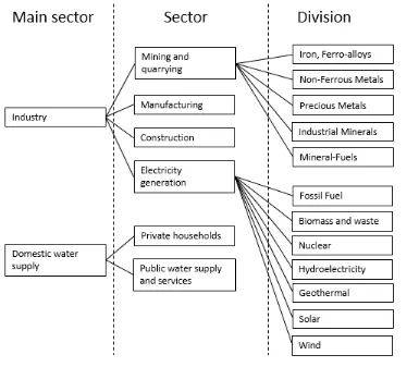
According to the hypothesis of this research, there are differences in water footprint between industrial sectors. A certain classification is needed for the main industrial sectors and domestic water supply to make different water footprints comparable within the industry.

The United Nations (2016c) designed an international standard industrial classification of all economic activities (ISIC). This classification contains a broad hierarchical structure of 21 sectors each consists of several divisions. These divisions consist of several groups and so on. The Organisation for Economic Co-operation and Development (OECD) and the database of UNdata (United Nations, Statistics Division, 2016a) use this classification and provide the gross added value per sector for most of the countries and years (OECD, 2017). The gross added value per sector is relevant for estimating the water consumption per country according to the method presented in chapter 2.2.

The water withdrawal of four industrial sectors is estimated for several countries and available at the database of Eurostat (Förster, 2016). Eurostat uses the NACE Rev.2 statistical classification of economic activities in the European community. NACE REV.2 classification is a derived classification from ISIC on EU-level. Several types of data, like water withdrawal, and gross added value for the main industrial sectors, are available and collected by Eurostat for the following industries:

 Mining and quarrying

 Manufacturing

 Electricity

 Construction

The definition of these specific sectors is abstracted from ISIC revision 4. These four sectors contain several divisions. The water consumed in these divisions together is the water footprint of a sector.

2.1.1

Mining and quarrying

Mining and quarrying include the extraction of minerals occurring naturally as solids (coal and ores), liquids (petroleum) or gases (natural gas). Extraction can be achieved by different methods such as underground or surface mining, well operation, seabed mining (United Nations, Department of Economic and Social Affairs, 2008). Mining and quarrying also include supplementary activities aimed at preparing the crude materials for marketing, for example crushing, grinding, cleaning, drying, sorting, concentrating ores, liquefaction of natural gas and agglomeration of solid fuels (United Nations, Department of Economic and Social Affairs, 2008).

This sector does not include the processing of the extracted materials which also covers the bottling of natural spring and mineral waters at springs and wells or the crushing, grinding or otherwise treating different kind of earth, rocks and minerals not carried out in conjunction with mining and quarrying. This is part of the section manufacturing (United Nations, Department of Economic and Social Affairs, 2008).

5 Australia through the tropics and to the sub-arctic conditions of Canada and Finland (Northey, Mudd, Saarivuori, Wessman-Jääskeläinen, & Haque, 2016). Mining could be considered one of the most diverse industries with respect to how it interacts with water resources (Younger, Banwart, & Hedin, 2002).

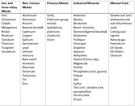
The mineral raw materials which can be produced by mining and quarrying is arranged in five divisions based on their chemical characteristics by the International Organizing Committee for the World Mining Congresses and is presented in Table 1 (Reichl, Schatz, & Zsak, World Mining Data, 2017).

Iron and Ferro-Alloy Metals

Non- Ferrous Metals

Precious Metals Industrial Minerals Mineral Fuels

Iron Chromium Cobalt Manganese Nickel Niobium Tantalum Titanium Tungsten Vanadium Aluminum Antimony Arsenic Bauxite bismuth Cadmium Copper Gallium Germanium Lead Lithium mercury Rare earth minerals Rhenium Selenium Tellurium Tin Zinc Gold, Platinum-group metals (palladium, platinum, rhodium) Silver Asbestos Baryte, Bentonite Boron minerals Diamond(gem/industrial) Diatomite Feldspar Fluorspar Graphite Gypsum Anhydrite Kaolin (China-clay) Magnesite Perlite

Phosphates (incl. guano) Potash

Salt Sulfur

Talc (incl. steatite and pyrophyllite)

Vermiculite Zircon

Steam coal (incl. anthracite and sub-bituminous coal) Coking coal Lignite Natural gas Petroleum Oil Sands Oil Shales Uranium

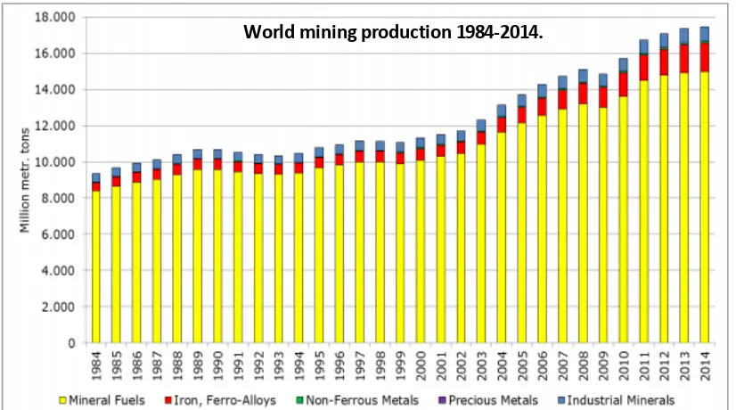
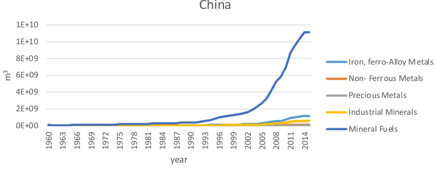
6 Figure 1 (Reichl, Schatz, & Zsak, World Mining Data, 2016) shows a distribution with a significant part of mineral fuels which dominates the world mining production.

Fi gure 1 Worl d mining production 1984-2014 by groups of minerals Reichl et al. (2016).

2.1.2

Manufacturing

Manufacturing includes the physical or chemical transformation of materials, substances, or components into new products, although this cannot be used as the single universal criterion for defining manufacturing. The materials, substances, or components transformed are raw materials that are products of other manufacturing activities. Substantial alteration, renovation or reconstruction of goods is generally considered to be manufacturing (United Nations, Department of Economic and Social Affairs, 2008).

According to UN Department of Economic and Social Affairs (2008), “Units engaged in manufacturing are often described as plants, factories or mills and characteristically use power-driven machines and materials-handling equipment. However, units that transform materials or substances into new products by hand or in the worker’s home and those engaged in selling to the general public of products made on the same premises from which they are sold, such as bakeries and custom tailors, are also included in this section. Manufacturing units may process materials or may contract with other units to process their materials for them. Both types of units are included in manufacturing.”

2.1.3

Electricity generation

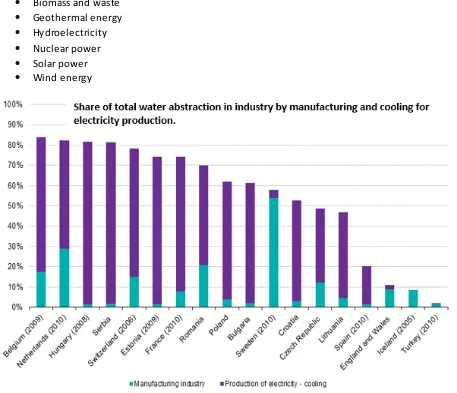
The electricity generation sector abstracts the most freshwater of all sectors in the industry in most countries (Shiklomanov, 2003). Figure 2 (Förster, 2016) shows the major contribution of the water abstraction by the production of electricity-cooling in Europe (Förster, 2016). Energy production requires significant volumes of fresh water and has significant impacts on water resources through thermal and chemical pollution. The largest water footprint is produced by hydropower and bioelectricity (Mekonnen, Gerbens-Leenes, & Hoekstra, 2015). Thermal power generation is responsible for a significant part of water abstraction in the electricity sector. For the USA 76% of the total water abstracted was needed for thermal power generation. In thermal power production, 0.5-3.0% of the water abstraction is consumed. (Shiklomanov, 2003). Besides thermal power, there are

7 different sources of electricity generation. A classification, used by US Energy Information Administration (EIA), will be used in this research (U.S. Energy Information Administration, 2014).The divisions used by the US EIA for the electricity generation sector are:

 Fossil fuels

 Biomass and waste

 Geothermal energy

 Hydroelectricity

 Nuclear power

 Solar power

 Wind energy

Fi gure 2 Share of total abstraction in the industry for the manufacturing industry and production of electricity (mainly cooling), 2011 (%) (Förster, 2016).

Electricity from fossil fuel, biomass, nuclear power

It is estimated how much water different kinds of power plants withdraws and how much water will be consumed in the process. The Food and Agriculture Organization of the United Nations (FAO) provide these indicators for different power plants which are shown in Table 2 (Kohli & Frenken, 2011).

Power plant and cooling system type Withdrawal (m3_MWh-1₎

Consumption (m3_MWh-1₎

Fossil fuel, biomass, waste once-through cooling 76-190 1.0 Fossil fuel, biomass, waste closed-loop cooling 2.0-2.3 2.0 Nuclear steam once-through cooling 95-230 1.5 Nuclear steam closed-loop cooling 3.0-4.0 3.0

Ta bl e 2 Wa ter withdrawal i ndicators for different sort of power plant cooling s ystems a ccording to the FAO (Kohli &

8 Averages from Table 2 are used when estimating the water abstraction and consumption of the division electricity from fossil fuel, biomass and waste, and electricity from nuclear power. Biomass and waste consume more water per megawatt-hour (MWh). According to the US EIA biomass is defined as organic materials of biological origin constituting a renewable energy source such as biodiesel, biofuels, biomass waste, densified biomass, fuel ethanol, wood, and wood-derived fuels (U.S. Energy Information Administration, 2014). It is estimated that this division consumes 20.016 m3_MWh-1 _{(Gerben-Leenes et al., 2008a).}

Hydroelectricity

There was a lot questioning about the water abstraction and consumption of hydropower generation (Mekonnen & Hoekstra, 2011c), (Bakken, Killingtveit, England, Alfredsen, & Harby, 2013). Hydroelectricity has historically been considered as a non-consumptive water user however, the study of 35 sites finds that, in contrary, hydropower is a large consumptive user of water (Mekonnen & Hoekstra, 2011a). A range between 1.08 m3_MWh-1 _{to 3045.6 m}3_MWh-1 _{with an average of 244.8}

m3_MWh-1 _{is estimated as water consumption by Mekonnen and Hoekstra (2012). In a more recent}

research, 54.35 m3_MWh-1 _{is estimated (Mekonnen et al., 2015). To estimate the total amount of}

consumed water the 54.35 m3_MWh-1 _{can be multiplied by the amount of generated electricity in MWh.}

The large range of consumption depends on the surface of the lake, the depth and the climate where the power is generated. In recent research the water consumption per country caused by hydropower is determined (Hogeboom, Knook, & Hoekstra, 2017). The water consumption per MWh of the corresponding country is used in this research, if not the average of 54.35 m3_MWh-1 _{is used.}

Geothermal

Geothermal electricity generation is projected to upcoming besides other renewable power generation sources (Clark, Harto, Sullivan, & Wang, 2010). It could grow even more if enhanced geothermal systems (EGS) technology, which can effectively operate on more broadly available lower-temperature geofluids, proves to be a good cost and environmental performer. Also, geothermal plants tend to run trouble-free at or near full capacity for most of their lifetimes (Clark et al., 2010). Geothermal power plants consume relatively less water per MWh energy output than other electric power generation technologies. The water footprint is estimated at 1.206 m3_MWh-1 _{(Mekonnen et al.,}

2015). However geothermal power plants can require (withdraw) around 7.6 m3_MWh-1 _{of water for}

cooling purposes (Clark et al, 2010). Solar energy

Solar energy can be utilized in three ways according to Gerben-Leenes et al.(2008a). Heat production, electricity production through photovoltaic (PV) cells, and electricity production through solar thermal power plants. It is estimated that on average 1.08m3_MWh-1 _{is consumed by using solar energy to}

generate electricity (Mekonnen et al., 2015). Wind energy

Wind energy utilizes the kinetic energy in the air to generate electricity. In wind farms, the average, annual energy generated varies between 0.05 and 0.25 GJm-2_{(Gerben-Leenes et al., 2008a). Wind}

9

2.1.4

Construction

This sector includes general construction and specialized construction activities for buildings and civil engineering works. “It includes new work, repair, additions and alterations, the erection of prefabricated buildings or structures on the site and also the construction of a temporary nature. General construction is the construction of entire dwellings, office buildings, stores and other public and utility buildings, farm buildings or the construction of civil engineering works” (United Nations, Department of Economic and Social Affairs, 2008).

In the construction sector, the direct water footprint is small compared with the indirect water footprint related to the mining and manufacturing of materials used in construction (Hoekstra A. Y., 2015). The direct water abstraction in the construction process is maximally 1 m3 _{per square meter of}

gross floor area. It has to be noted that the figures cited here refer to gross blue water abstraction, not net water consumption (McCormack, Treloar, Palmowski, & Crawford, 2007).

For Great Britain, the average water consumption at the construction site is estimated for the year 2008. In their research, they found that the average tap water consumption is 148m3 _{per £ million}

contractors output at a constant price according to the Strategic Forum Water Subgroup. (Waylen, Thornback, & Garett, 2011).

2.1.5

Classification Domestic water supply

Domestic water supply means the source and infrastructure that provides water to households and public, commercial and municipal needs (Perlman, 2017). Municipal water abstraction includes abstraction of water and its treatment and distribution mostly for domestic purposes to cities and towns and to public and private enterprises (Shiklomanov, 2003). The public water supply also includes water for industry, which consumes high-quality fresh water from the city water supply systems. A significant part of the domestic water consumption is used for watering lawns and gardens in certain countries (Shiklomanov, 2003).

Domestic or municipal water supply is also defined by Aquastat (2017) in their glossary as “the annual quantity of water withdrawn primarily for the direct use by the population. It include s water from primary renewable and secondary freshwater resources, as well as water from over-abstraction of renewable groundwater or withdrawal from fossil groundwater, direct use of agricultural drainage water, direct use of (treated) wastewater, and desalinated water. It is usually computed as the total water withdrawn by the public distribution network. It can include that part of the industries and urban agriculture, which is connected to the municipal network.” (Food and Agriculture Organization of the United Nations, Aquastat, 2017)

For the domestic water supply sector, a consumptive portion of 10% is used in previous research (Mekonnen & Hoekstra, 2011a). A consumptive portion of 10-20% is estimated in the World Water Report (United Nations, 2009).

Different purposes of the water abstraction in the domestic water supply leads to a classification in sectors. In the Eurostat databases the domestic water supply is classified in the following sectors (Eurostat, 2017):

• Water abstraction for private households

• Water abstraction for public water supply and services

10 due to evaporation, leakage in water supply and sewer systems, and water used for gardening, cleaning streets, for recreational areas, and allotments. These causes of water consumption are not part of the sector private households.

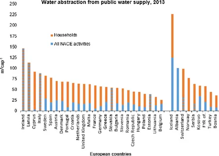
Figure 3 shows that households constitute a significant part of the abstraction from the public water supply. The industrial sectors are responsible for the other part of the water abstraction (Eurostat, 2015). Public supply refers to water withdrawn by public and private water suppl iers that provide water at least 25 people or have a minimum of 15 connections (U.S. Geological Survey, 2009). All other activities from the 21 derived sectors of ISIC with commercial purposes which uses public water supply fall within this sector. Small industries and services who abstracts tap water are part of this sector. According to Figure 3, these industries and services abstract a relatively small volume of tap water compared to households. Therefore, industries, services public (ISIC activities) and municipal which abstracts from tap water can be classified as one sector.

Fi gure 3 Wa ter a bstraction from the public water s upply i n m3 _{per inhabitant for European countries, NACE a ctivities a re the}

EU equi va l ent of the ISIC cl a s s i fi ca ti on 2013 (Eurostat, 2015).

Eurostat is the only database who distinguished different divisions in the domestic water supply. Besides, Eurostat provides a low amount of annual data for both divisions. In addition, it is only data about abstraction for a marginal amount of countries and years. Due to this lack of data and literature, the domestic water supply sector will be considered as one sector in this research. The distinction between private households and public water supply and services is not been made.

2.1.6

Overview classification

11 and electricity generation sector. Also, the water footprint of electricity generation is estimated. And only the water footprint of the main sector domestic water supply is estimated instead of its sectors.

Fi gure 4 Overvi ew of the sectors a nd di vi s i ons rel eva nt for the es ti ma ti on of the wa ter footpri nts i n thi s res ea rch.

2.2

The blue water footprint

This section provides the method of estimating the blue water footprint per country of each industrial sector and the domestic water supply sector annually for the period 1960-2015. Each sector, classified in section 2.1, consists of several divisions with each its own blue water footprint. The total blue water footprint of a sector is a combination of blue water footprints of the divisions. If possible, a weighted average of water consumption is obtained per sector by using available data about the quantities produced in the divisions. Some sectors have a significantly large part in water consumption in the industry. For the electricity generation sector, the water footprint is therefore estimated per division. The average water consumption per division is obtained by estimating the average water footprint of the groups who form a division together in m3_t-1 _{in the industrial sector. Otherwise, an estimation is}

made by looking at the worldwide distribution to obtain a weighted average of water consumption of the divisions, like the mining and quarrying industry.

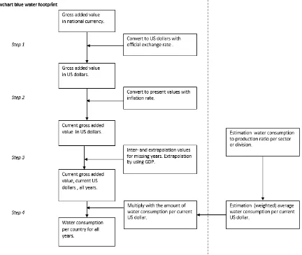
12 countries. It is annual data for as long as it is available in the period 1960-2015. The gross added value measures the contribution to an economy of an individual producer, industry, sector or region (Financial Times, 2017). This data is first converted to current US dollars if it has not been done yet. Therefore, several steps are done to convert these yearly values to the blue water footprint. While estimating the averages for each sector several assumptions are made, depending on the data availability, on different detail level. Assumptions cause rougher estimates of the water footprints of some of the industrial sectors. It is unavoidable on this scale of research. Accepting these assumptions, a rough estimate of the water consumption in the smaller divisions and groups is applicable to estimate the water footprint per country per sector and year.

Figure 5 shows the flow diagram of the method which is followed while estimating the blue water footprint per sector. However, this flowchart forms the basis of estimating the blue water footprint but it can differ per sector. This method is used to estimate the blue water footprint of the mining and quarrying sector and the construction sector. Step one and two are skipped when the blue water footprint of the manufacturing industry was estimated. The blue water footprint of the electricity generation divisions is estimated only using step four and not with a water consumption ratio per current US dollar but with a water consumption ratio per MWh.

The flowchart starts with indicating the blue water footprint per current US dollar and eventually estimating the blue water footprint for a sector per year per country.

Step 1: The gross added value from the UN Statistical Division is given in the local currency of the corresponding country for most of the sectors. This currency is converted to United States Dollars (US dollar). The World Bank (2017) maintains a databank which contains official exchange rates for countries for most of the years in the period 1960-2015. Accordingly, all values are converted to US dollars.

Step 2: The data is given in US dollars but needs to be converted to current US dollars. The present value is estimated by using the inflation rate for each country and each year which is abstracted from The World Bank (2016). The present value is calculated by the present value formula (Averkamp, 2017). This formula is used in finance and calculates the present day value of an amount that is received at a future or past date.

𝑃𝑟𝑒𝑠𝑒𝑛𝑡 𝑉𝑎𝑙𝑢𝑒 =𝑉𝑎𝑙𝑢𝑒

(1+𝑖)𝑛 (1)

13

Fi gure 5 Fl ow cha rt of the bottom-up a pproa ch to es ti ma ti ng the bl ue wa ter footpri nt of a s ector.

Step 3: The United Nations Statistical Division and the US Energy Information Administration does not have data for each particular year for the mining and quarrying, construction, manufacturing, and electricity generation industry. Missing values are interpolated or extrapolated after step two. Linear interpolation is used between two known values. The Gross Domestic Product (GDP) extracted from the World Bank (2017) of the corresponding country is used to extrapolate missing GAV values. The growth factor of the GDP between two consecutive years is estimated for each country. When GDP data is not available for a country the growth factor is used of the worldwide GDP. For recently formed countries the GDP is used of the former country like the former USSR countries and Yugoslavia. Step 4: The GAV in current US dollars is at this step multiplied by the water consumption per current US dollar of the corresponding industrial sector. The water consumption per current US dollar is estimated in different ways. It is sector dependent how the water consumption per current US dollar is estimated. This can be seen in the following sections about the sectors.

14

2.2.1

Mining and Quarrying

The United Nations Statistics Division provides data about the gross value added for most of the countries for each industrial sector according to the ISIC rev.4 classification. This data spans the whole mining and quarrying sector. With this data, the flowchart in Figure 5 is followed. The economical share of the different mining and quarrying divisions is extracted from World Mining Data, for the year 2015 (Reichl et al., 2017). It is estimated how much, in tons and in value, of a mining and quarrying division is produced. After estimating the water consumption per mining group per current US dollar, the weighted average water consumption per division is estimated, continued by the estimation of the weighted average water consumption of the mining and quarrying sector. In the flowchart, the estimation of the water consumption per US dollar is seen on the right side of the diagram and leads to step four.

The distribution of the mining and quarrying sector is obtained for the year 2015 in the report of the world mining data (2017). Distribution is defined as the composition, based on economic value or weight in tons, of the mining and quarrying sector by different mining and quarrying divisions. Table 3 shows the distribution, and just like in Figure 1 it can be concluded that the mineral-fuels have the largest contribution.

Country Iron, ferro-alloys

Non-ferrous metals

Precious metals

Industrial minerals

Mineral-fuels

Share of production in tons 9.2% 0.5% 0.0% 4.4% 84.1%

Share of value in US dollars 7.7% 6.9% 3.9% 2.4% 75.2%

Ta bl e 3 Distribution of the mining products in percentages of the production in metric tons and in the value of US dollars (Rei chl et al., 2017).

According to the world mining report the six biggest producers, China, USA, Russia, Australia, India, and Saudi Arabia are responsible for of 60% of the total world production. They are also responsible for 50% of the value of the total mining production in 2015 (Reichl et al., 2017). For that reason, the water footprint of the six largest producers is estimated for each division of the mining and quarrying sector.

It can be justified by the fact that the water footprint of a single division of one of the six largest producers can be larger than the total production of many other countries. Besides, the distribution of one of the six biggest producers differs compared to the average distribution of the world mining production. This will results in a larger margin of error when estimating the water footprint by using the distribution of the world mining and quarrying production instead of the distribution of the country itself.

15

Country Total (tons mill US dollar -1₎

Iron, ferro-alloys Non-ferrous metals Precious metals Industrial minerals Mineral-fuels

China 7.05*103 _1.18*104 _5.13*102 _{0.22 1.056*10}4 _8.39*103

United States 5.40*103 _1.06*104 _3.31*102 _{0.15 1.14*10}4 _5.54*103

Russia 4.85*103 _4.26*103 _4.60*101 _{0.15 2.13*10}3 _5.28*103

Australia 6.89*103 _1.18*104 _4.03*104 _{0.15 9.14*10}3 _8.06*103

India 7.65*103 _5.51*103 _5.65*102 _{1.62 1.07*10}4 _9.54*103

Saudi Arabia 2.87*103 _1.82*104 _5.24*102 _{0.06 5.00*10}4 _2.86*103

total world 3.27*103 _4.30*103 _3.29*102 _{0.20 9.14*10}4 _3.40*103

Ta bl e 4 the a mount of ton of a mi ning a nd quarrying product i n 2015 to be produced for a va lue of 1 mi llion US dollars for the s ix biggest producers in mining and for the world (Reichl et al., 2017). The first column represents the average of all mining products i n tons per country to produce for a va l ue of 1 mi l l i on US dol l a rs .

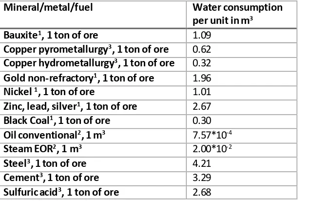
The amount of tons produced for a certain mining product is multiplied with the consumption to production ratio. The amount of water consumed to produce several mining and quarrying products are given in Table 5. These are products and minerals in the mining and quarrying sector, the values are gained from several reports; bauxite, nickel, zinc, lead, silver, gold non-refractory (Hoekstra 2015), oil conventional, steam EOR (Clark et al.,2010), copper pyrometallurgy and hydrometallurgy, cement and sulfuric acid (Northey et al., 2016). The products in Table 5 are subdivided into the mining and quarrying divisions distinguished by the report of the world mining data (Reichl et al., 2017).

Mineral/metal/fuel Water consumption per unit in m3 Bauxite1_{, 1 ton of ore 1.09}

Copper pyrometallurgy3_{, 1 ton of ore 0.62} Copper hydrometallurgy3_{, 1 ton of ore 0.32} Gold non-refractory1_{, 1 ton of ore 1.96} Nickel 1_{, 1 ton of ore 1.01} Zinc, lead, silver1_{, 1 ton of ore 2.67} Black Coal1_{, 1 ton of ore 0.30} Oil conventional2_{, 1 m}3 _7.57*10-4

Steam EOR2_{, 1 m}3 _2.00*10-2

Steel3_{, 1 ton of ore 4.21} Cement3_{, 1 ton of ore 3.29} Sulfuric acid3_{, 1 ton of ore 2.68}

Ta bl e 5 Consumption to production ra tio for mining products.

1. (Hoekstra A. Y., The wa ter footprint of i ndustry, 2015) 2. Cl a rk, Ha rto, Sullivan & Wa ng, 2010) 3. (Northey, Mudd, Sa a rivuori, Wessman-Jääskeläinen & Ha que, 2016).

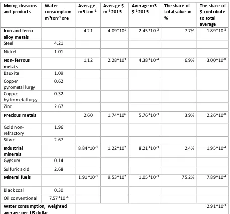
For the six most producing countries in this sector, the corresponding distribution of the divisions is used for estimating the blue water footprint per division, based on the distribution of the year 2015. The distribution of the economic shares per division of the total economic value of mining and quarrying is given in Table 6. This share is multiplied by the average value in current US dollars per m3

consumed per mining and quarrying group. The value is summed and represents the weighted average water consumption for the whole mining and quarrying sector, by using the amount of water consumed per current US dollar and the share of the mining product and mining group worldwide based on mining data of 2015 (Reichl et al., 2017). According to Table 6, an average of 2.91*10-3 _m3 _is

16

Mining divisions and products

Water consumption m3_ton-1 _ore

Average m3 ton-1

Average $ m-3 ₂₀₁₅

Average m3 $-1 ₂₀₁₅

The share of total value in %

The share of $ contribute to total average Iron and

ferro-alloy metals

4.21 4.09*101 _2.45*10-2 _{7.7% 1.89*10}-3

Steel 4.21

Nickel 1.01

Non- ferrous metals

1.12 2.28*103 _4.38*10-4 _{6.9% 3.00*10}-8

Bauxite 1.09

Copper pyrometallurgy 0.62 Copper hydrometallurgy 0.32

Zinc 2.67

Precious metals 2.60 1.74*106 _5.76*10-3 _{3.9% 2.26*10}-8

Gold non-refractory

1.96

Silver 2.67

Industrial minerals

8.84*10-1 _1.22*102 _8.21*10-3 _{2.4% 1.95*10}-4

Gypsum 0.14

Sulfuric acid 2.68

Mineral fuels 1.91*10-1 _9.53*102 _1.05*10-3 _{75.2% 7.89*10}-4

Black coal 0.30

Oil conventional 7.57*10-4

Water consumption, weighted average per US dollar

2.91*10-3

Ta bl e 6 Wei ghted a vera ge wa ter cons umpti on per US dol l a r for Mi ni ng a nd qua rryi ng di vi s i ons .

2.2.2

Manufacturing

The manufacturing industry is a very diverse industry with 23 varying divisions. Consequently, the method presented in the flowchart in Figure 5 is more difficult to use in this case because averaging the water consumption per ton of all these products together will be less representative of this sector. A different approach is used for this sector to estimate the water abstraction, not to be confused with water consumption, per current US dollar. Eurostat (2017) provides data about water abstraction in the manufacturing industry for several countries for several years. The World Bank (2016) provides for this sector the gross added value for each country and years in current US dollar. Accordingly, the water abstraction per current US dollar is estimated for these countries. All these values are averaged and give a water abstraction of 3.67*10-2 _m3 _{per current US dollar.}

17 manufacturing industry of Canada is used as a representative water consumption to withdrawal ratio to estimate the blue water footprint for other countries and for each year.

Step 1 and 2 of the flowchart is excluded from this sector because the GAV is already in current US dollar provided by the World Bank (2016). After interpolation and extrapolation in step 3, and estimating the water consumption per current US dollar, step 4 is completed.

2.2.3

Electricity generation

The electricity generation sector use a slightly different method as presented in the flowchart in Figure 5.

Due to large water abstraction in the electricity generation sector, the water footprint for different sources of electricity is estimated. This sub-classification of electricity sources is used by the US Energy Information Administration (2014) and are treated as divisions in this research. The amount of consumption per MWh per source is shown in Table 7.

Source Consumption M3_MWh-1

Fossil fuel1) _1.50

Biomass and waste(3) _20.02

Nuclear(1) _2.25

Hydroelectricity(2) _{54.35 (Averaged)}

Geothermal(2) _1.21

Solar(2) _1.08

Wind(2) _7.2*10-4

Ta bl e 7 Amount of water consumed to generate 1 MWh per energy s ource.

1: (Kohl i & Frenken, 2011) 2: (Mekonnen, Gerbens-Leenes, & Hoekstra, 2015) 3: (Gerbens-Leenes, Hoekstra, & Va n der Meer, 2008b).

For almost every country, the US EIA provides data from 1980 to 2014 about the amount of Mega Watthour (MWh) generated per source. The blue water footprint is therefore estimated in a different way than the other sectors. For the period 1960-1980, there is no data available from the US EIA. Missing data is extrapolated by using the GDP.

Eventually, the blue water footprint is estimated by multiplying the water consumption per MWh of the corresponding source, instead of current US dollar. For Hydroelectricity, the water footprint per MWh is estimated for a significant amount of the countries (Hogeboom et al., 2017). Therefore the corresponding water footprint per MWh is used, if not the average of 54 m3 _{per MWh is used}

(Mekonnen et al., 2015).

2.2.4

Construction

Similarly, as for the mining and quarrying sector, the United Nations Statistics Division (2016a) provides the gross added value for almost every country for multiple years for this specific industrial sector. The blue water footprint is estimated by using exactly the flowchart in Figure 5.

For Great Britain, it is estimated what the average tap water consumption on site is. As tap water is mostly used in construction, these values are used in this research. 2008 Is used as a baseline in the report: WATER: An Action Plan for reducing water usage on construction sites (2011). In this report, they found that the average tap water consumption is 148m3 _{per £ million contractors output at a}

18

2.2.5

Domestic water supply

The domestic water supply is considered as one sector and will be estimated by a different method as shown in Figure 4.

The United Nations quoted in their World Water Development Report 2016: Water and Jobs (2016b) an estimate of the consumptive factor which is between 10% and 20% for domestic use (Margat & Andréassian, 2008). The average, 15%, is used to estimate the water consumption of all countries and years, this fraction is also used in other literature by Vandecasteele, Bianchi, Basitta e Silva, Lavelle, and Batelaan (2014).

The total water abstraction in the domestic water supply is available in the database of the FAO, (Food and Agriculture Organization of the United Nations, Aquastat, 2017) . Although missing values are linearly interpolated and extrapolated by using GDP to gain values for the whole period and for each country. These values are multiplied by the water consumption to withdrawal ratio and provide the estimated water footprint of domestic water supply.

2.3

The grey water footprint

The grey water footprint is an indicator of the water volume needed to assimilate a pollutant load that reaches a water body. The grey water footprint is based on the tier-1 level. Tier 1 simply uses a leaching-runoff fraction to translate data on the amount of a chemical substance applied to the soil to an estimate of the amount of the substance entering the groundwater or surface water system (Franke, Boyacioglu, & Hoekstra, 2013).

The part of the return flow which is disposed into the environment without prior treatment can be taken as a measure of the grey water footprint. The so-called dilution factor represents the number of times that the effluent volume has to be diluted with ambient water in order to arrive at the maximum acceptable concentration level (Hoekstra et al., 2011). The dilution factor 1 is a very conservative factor to be applied for all untreated return flows of the industry and domestic water supply. Based on literature and the equation below a new dilution factor is estimated per sector if possible.

A simplified equation of the grey water footprint is the following (Hoekstra et al., 2011): 𝑊𝐹𝑔𝑟𝑒𝑦 =

𝑐𝑒𝑓𝑓𝑙−𝑐𝑎𝑐𝑡

𝑐𝑚𝑎𝑥−𝑐𝑛𝑎𝑡× 𝐸𝑓𝑓𝑙𝑐,𝑡 (2)

Where 𝑐𝑒𝑓𝑓𝑙−𝑐𝑎𝑐𝑡

𝑐𝑚𝑎𝑥−𝑐𝑛𝑎𝑡 is the dilution factor.

𝑐𝑒𝑓𝑓𝑙 is the concentration of the contaminant in the effluent in mg l-1.

𝑐𝑎𝑐𝑡 is the concentration of the contaminant in the current stream, before abstraction in mg l-1. 𝑐𝑚𝑎𝑥 is the maximum allowable concentration of the contaminant in the surface water in mg l-1. 𝑐𝑛𝑎𝑡 is the natural concentration of the contaminant in surface waters in mg l-1 .

𝐸𝑓𝑓𝑙 is the part of the abstracted water returning to the surface water in m3_y-1 _{where c is country}

and t is time in years.

In this research, 𝑐𝑎𝑐𝑡 is equal to 𝑐𝑛𝑎𝑡 because characteristics of individual streams and surface water will not be used and therefore only the natural concentration worldwide.

2.3.1

Mining and Quarrying

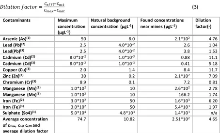
19 open cast, as well as underground coal, is mined according to Prasad, Kumari P, Shamima and Kumari S (2013). Metal mines in the surrounding of streams can cause heavy metal contamination of surface water (Schaider, Senn, Estes, Brabander, & Shine, 2014). Most frequently substances that pollute water are caused by different mining divisions. These substances are arsenic, lead, cadmium, copper, zinc, chromium, manganese, iron, and sulphates. Concentrations of these substances are found in varying degrees in ground and surface water nearby mines in different cases. The maximum allowable concentrations and natural concentrations of these contaminants are given in the Canadian Environmental Quality Guidelines by CCME (2013). In Table 8 the substances are given with maximum, natural and found concentrations nearby mining areas in ground and surface water (Prasad et al.,2013), (Schaider et al., 2014), (Razo, Carrizales, Castro, Diaz-Barriga, & Monroy, 2003). In this research the scope lies on the grey water footprint of a sector, therefore an average of all maximum, natural and found concentrations are made to estimate an average dilution factor for the mining and quarrying industry, also shown Table 8.

The dilution factor is estimated by the following calculation (Mekonnen & Hoekstra, 2011a): 𝐷𝑖𝑙𝑢𝑡𝑖𝑜𝑛 𝑓𝑎𝑐𝑡𝑜𝑟 =𝐶𝑒𝑓𝑓𝑙−𝐶𝑎𝑐𝑡

𝐶𝑚𝑎𝑥−𝐶𝑛𝑎𝑡 (3)

Contaminants Maximum

concentration (μgL-1₎

Natural background concentration (μgL-1₎

Found concentrations near mines (μgL-1₎

Dilution factor(-)

Arsenic (As)(1) _{50 8.0 2.1*10}2 _4.76

Lead (Pb)(2) _{2.5 4.0*10}-2 _{2.6 1.04}

Lead(Pb)(3) _{2.5 4.0*10}-2 _{3.8 1.53}

Cadmium (Cd)(2) _8.0*10-2 _1.0*10-3 _{0.88 11.1}

Cadmium (Cd)(3) _8.0*10-2 _1.0*10-3 _{0.41 5.18}

Copper (Cu)(3) _{2.0 1.4 8.4 11.7}

Zinc (Zn)(3) _{30 0.2 2.1*10}2 _7.09

Chromium (Cr)(3) _{8.9 0.1 7.2 0.81}

Manganese (Mn)(2) _1.0*102 _{10 2.6*10}2 _2.78

Manganese (Mn)(3) _1.0*102 _{10 166.2 1.74}

Iron (Fe)(2) _3.0*102 _{50 1.6*10}3 _6.20

Iron (Fe)(3) _3.0*102 _{50 5.4*10}3 _1.97

Sulphate (So4)(3) _5.0*104 _4.8*103 _1.4*103 _n/a

Average concentration of cmax, cnat ceffl and

average dilution factor

74.7 10.82 2.51*102 _4.65

Ta bl e 8 Ni ne substances who pollutes s urface and groundwater near mining a reas a ccording to s everal types of research. The a verage dilution factor i s estimated. Found concentrations near mines are a bstracted from the following research: 1. Ra zo, Ca rrizales, Ca stro, Diaz-Barriga, a nd Monroy, (2003) 2. Scha ider, Senn, Es tes, Bra bander, & Shi ne (2014) 3. Pra sad et a l . (2013).

The grey water footprint is estimated by multiplying the dilution factor with the annual water abstraction for each country. The water consumption per country is already estimated as the blue water footprint. The water abstraction minus the water consumption is the effluent which is needed to estimate the grey water footprint.

20 the average water abstraction per current US dollar times the gross added value of the mining and quarrying industry.

The grey water footprint is estimated by:

𝐺𝑟𝑒𝑦 𝑊𝐹 = 𝐷𝐹 × (𝑡𝑜𝑡𝑎𝑙 𝑤𝑎𝑡𝑒𝑟 𝑎𝑏𝑠𝑡𝑟𝑎𝑐𝑡𝑖𝑜𝑛𝑐,𝑡− 𝑡𝑜𝑡𝑎𝑙 𝑤𝑎𝑡𝑒𝑟 𝑐𝑜𝑛𝑠𝑢𝑚𝑝𝑡𝑖𝑜𝑛𝑐,𝑡) (4) Where DF is dilution factor, c is country and, t is time in years. The grey water footprint for the six most

producing countries in this sector is estimated by the same method as other countries. The grey water footprint cannot be estimated per division of the mining and quarrying sector because it is not clear in literature in what kind of mining and quarrying division which contaminants occur and the quantities of those contaminants. Therefore, the averaged dilution factor 5 will be used for the top six producing countries in this sector.

2.3.2

Manufacturing

As stated in section 1.2, the manufacturing industry is a very diverse industry with 23 varying divisions. Wastewater from manufacturing processes released into streams, rivers, and lakes adds pollutants to the water. Other water pollution occurs when tanks storing chemicals leak and leach into the groundwater. Paper and textile manufacturing, which use chemicals such as chlorine and benzene, are among the processes that can contribute to water pollution (Myers, 2016). A weighted average as a dilution factor will, because of the diversity of this sector, not be representative of the manufacturing industry. Besides, the load of the effluent of manufacturing industries is not known in the literature. The conservative dilution factor of 1 is used for the industrial (Mekonnen & Hoekstra, 2011a). Therefore the grey water footprint is estimated by multiplying the effluent of the manufacturing sector with this dilution factor 1 for each year and country.

2.3.3

Electricity generation

The electricity generation divisions, which includes thermal and nuclear power plants, are by far the divisions which abstract the most water. Those divisions generate electricity by fossil fuels, nuclear power and biomass and waste. It is estimated how much water is abstracted in these divisions per MWh in chapter 1.3. These divisions pollute the water by the effluent with a different, higher, temperature. The thermal difference of the effluent water is the biggest form of pollution within these divisions. This results in a grey water footprint with a corresponding dilution factor.

Thermal and nuclear power plants discharge into rivers and lakes which are 8-12 degrees Celsius above ambient water temperature (Shiklomanov, 2003). To sustain the quality of fresh water, water temperature may increase with maximal three degrees Celsius (EU, 2006). With the following formula, the dilution factor can be calculated and thereby the grey water footprint (Hoekstra et al., 2011). 𝑊𝐹𝑔𝑟𝑒𝑦 =

𝑇𝑒𝑓𝑓𝑙−𝑇𝑎𝑐𝑡

𝑇𝑚𝑎𝑥−𝑇𝑛𝑎𝑡× 𝐸𝑓𝑓𝑙𝑐,𝑡 (5)

Where 𝑇𝑒𝑓𝑓𝑙−𝑇𝑎𝑐𝑡

𝑇𝑚𝑎𝑥−𝑇𝑛𝑎𝑡 is the dilution factor.

𝑇𝑒𝑓𝑓𝑙− 𝑇𝑎𝑐𝑡 is difference between the temperature in degrees Celsius of an effluent flow and the receiving water body.

𝑇𝑚𝑎𝑥− 𝑇𝑛𝑎𝑡 is the maximum temperature rise in degrees Celsius.

21 For power plants, the dilution factor is an average of 10 degrees Celcius divided by a maximum increase of 3 degrees. 10

3 = 3,3 is a rough estimation of the dilution factor for the thermal power plants by fossil fuels and biomass and waste and nuclear power plants.

Geothermal power plants can have impacts on the quality of water. Hot water pumped from underground reservoirs often contains high levels of sulfur, salt, and other minerals (Union of Concerned Scientists, 2016). The geothermal exploitation causes the drifting of contaminants such as mercury, antimony, boron, arsenic, and hydrogen sulfide (Manzo, Salvini, Guastaldi, Nicolardi, & Giuseppe, 2013). Concentrations of contaminants in the effluent are not quantified in literature. Therefore, the conservative approach of the dilution factor 1 is used to estimate the grey water footprint. The effluent per country and year of this division is multiplied by the dilution factor. Currently, there is no evidence in literature of pollution in fresh surface or ground water by solar electricity, wind-driven electricity and hydroelectricity generation. A contaminant load of their effluent is zero which results in no grey water footprint. It must be noticed the grey water footprint is only zero for operation phase. The construction phase of these different electricity generators could have a different grey water footprint but is not relevant to this research.

2.3.4

Construction

Sources of water pollution on building sites include diesel and oil, paints, solvents, cleaners and other harmful chemicals like construction debris, dirt, and cement (Gray, 2017). Due to a lack of literature about a load of water pollution caused by the construction industry, a conservative dilution factor of 1 is used for the effluent in the construction industry for all countries and years. This dilution factor is used for the industrial sector in the report of Mekonnen and Hoekstra (2011b).

2.3.5

Domestic water supply

Human emission in wastewater consists of the pollutant substances nitrogen (N) and phosphates (P). For estimating the grey water footprint, a load of these emissions needs to be estimated. The load divided by the difference between the ambient water quality standard for N or P (the maximum acceptable concentration 𝑐𝑚𝑎𝑥 mgL-1) and the natural concentration of N or P in the receiving water body (𝑐𝑛𝑎𝑡 in mgL-1) results in the grey water footprint. These concentrations are respectively 2.9 mgL -1 _{or 0.4mgL}-1 _{for N (Mekonnen & Hoekstra, 2015) and respectively 0.024 mgL}-1 _{and 0.01 mgL}-1 _{for P}

(Franke, Boyacioglu, & Hoekstra, 2013). 𝐺𝑟𝑒𝑦 𝑤𝑎𝑡𝑒𝑟 𝑓𝑜𝑜𝑡𝑝𝑟𝑖𝑛𝑡 = 𝐿𝑜𝑎𝑑

𝐶𝑚𝑎𝑥−𝐶𝑛𝑎𝑡 (6)

The load can be estimated by the following formula for nitrogen or phosphorus:

𝐿𝑜𝑎𝑑 = (𝐸𝑠𝑤× 𝐷(𝑐,𝑡) ∗ 𝑇𝑃(𝑐,𝑡) ) + ( 𝐸ℎ𝑢𝑚× (1 − 𝐷(𝑐,𝑡))× 𝑇𝑃(𝑐,𝑡))𝑓𝑠𝑤 (7)

Where 𝐸𝑠𝑤 is emission in N or P from the sewage for a country and year in kg-1cap-1y-1 , 𝐸ℎ𝑢𝑚 is de emission per from humans in kg-1_cap-1_y-1_{, 𝐷}

(𝑐,𝑡) is the fraction connected to sewerage system per country and year, 𝑇𝑃(𝑐,𝑡) is total population of a country and year (United Nations, 2017). Where 𝑓𝑠𝑤 is the non-sewered human waste that enter the surface water through dumping of human waste in open water or through surface runoff. This is assumed 10% (Mekonnen & Hoekstra, 2017). In total, this is the load of the emission which comes via the sewerage, the left the side of the formula, or direct from humans to surface water for each year and country, the right side of the formula. The total emission of N from sewerage is estimated with the following equation:

22 Where 𝐸𝑠𝑤𝑁 is the nitrogen emission to surface water in kg-1_cap-1_y-1_{, 𝐸}

ℎ𝑢𝑚𝑁 is the human nitrogen emission per country and year in kg-1_cap-1_y-1_{, D is the fraction of the total population that is connected}

to public sewerage systems (no dimension), and 𝑅𝑁 _{is the overall removal of nitrogen through} wastewater treatment (no dimension). These variables vary per world region and year and are provided in the research of Van Drecht, Bouwman, Harrison, and Knoop, (2009).

If available, country specific values are used for some years. The total population per country per year is obtained (United Nations, 2017). The nitrogen emission is estimated per year and per country and is based on the dietary per capita protein consumption which is abstracted from FAOSTAT (2018). The N intake through food is estimated by assuming an average of 16% N content in the protein consumed. About 97% of the N intake is assumed to be excreted in the form of urine and faeces and the remainder 3% is lost via sweat, skin, hair, blood, and miscellaneous (Mekonnen & Hoekstra, 2015). The percentage of population connected to public sewerage systems for several countries is abstracted from Eurostat (2016). Three wastewater treatment types with differing N removal efficiencies are based on the work of (Van Drecht et al., 2009). They distinguish primary treatment (10% N removal), secondary treatment (35% N removal) and tertiary treatment (80% N removal). Data on the distribution of these different treatment types are given by Van Drecht et al. (2009) on a regional scale and for several countries on a national scale (OECD, 2015). If data is available for these variables, but not for every year in the period 1960-2015, interpolation or extrapolation is used based on the world region data (Van Drecht et al., 2009).

The total emission of P from sewage is estimated with the following equation:

𝐸𝑠𝑤𝑃 = (𝐸ℎ𝑢𝑚𝑃 + 𝐸𝐿𝑑𝑒𝑡𝑃 + 𝐸𝐷𝑑𝑒𝑡𝑃 /𝐷)𝐷(1 − 𝑅𝑃) (9)

Where 𝐸𝑠𝑤𝑃 is the P emission to surface water in kg-1cap-1y-1, 𝐸ℎ𝑢𝑚𝑃 is the human P emission in kg-1cap -1_y-1_{, 𝐸}

𝐿𝑑𝑒𝑡𝑃 is the P emission from laundry detergents in kg-1cap-1y-1, 𝐸𝐷𝑑𝑒𝑡𝑃 the P emission from dishwasher detergents kg-1_cap-1_y-1_{, D is the fraction of the total population that is connected to public}

sewerage systems (no dimension), and 𝑅𝑃 _{is the overall removal of P through wastewater treatment} (no dimension). These variables vary per world region and year (Van Drecht et al., 2009). The P emission is estimated by using a ratio of 10:1 between N and P (Mekonnen & Hoekstra, 2017). The overall removal is estimated as a weighted average of primary, secondary and tertiary sewerage systems in the specific region for N and P based on data of Van Drecht et al. (2009). The amount of total population and the percentage of the population connected to waste water treatment is already obtained when the load of N is estimated and stays the same.