Model based clustering of non Gaussian panel data based on skew t distributions

University of Warwick institutional repository: http://go.warwick.ac.uk/wrap

This paper is made available online in accordance with

publisher policies. Please scroll down to view the document

itself. Please refer to the repository record for this item and our

policy information available from the repository home page for

further information.

To see the final version of this paper please visit the publisher’s website.

Access to the published version may require a subscription.

Author(s): Miguel A. JUÁREZ and Mark F. J. STEEL

Article Title: Model-Based Clustering of Non-Gaussian Panel

Data Based on Skew-t Distributions

Year of publication: 2010

Link to published article:

Model-based Clustering of non-Gaussian Panel Data Based on

Skew-

t

Distributions

Miguel A. Juárez and Mark F. J. Steel∗

University of Warwick

Abstract

We propose a model-based method to cluster units within a panel. The underlying model is autoregressive and

non-Gaussian, allowing for both skewness and fat tails, and the units are clustered according to their dynamic

behaviour, equilibrium level and the effect of covariates. Inference is addressed from a Bayesian perspective and

model comparison is conducted using Bayes factors. Particular attention is paid to prior elicitation and posterior

propriety. We suggest priors that require little subjective input and possess hierarchical structures that enhance

inference robustness. We apply our methodology to GDP growth of European regions and to employment growth

of Spanish firms.

keywords: autoregressive modelling; employment growth; GDP growth convergence; hierarchical prior;

model comparison; posterior propriety; skewness.

1 Introduction

Models for panel or longitudinal data are used extensively in economics and related disciplines (Baltagi, 2001;

Hsiao, 2003), as well as in health and biological sciences (Diggleet al., 2002; Weiss, 2005). Typically, panels are

formed according to some criteria (e.g.geographical, economical, demographical, etc.) with the intention of

gain-ing strength when estimatgain-ing quantities common to all individual units in the panel. However, this groupgain-ing may

strongly affect inference if presumed common characteristics of the units are, in reality, quite different. In these

cases, clustering units within the panel may prove useful. This will allow the units to share some common

para-meters, thus borrowing strength in their estimation, but to also have some cluster-specific parameters. In particular,

we will consider model-based clustering, which is based on a formal statistical framework (Banfield and Raftery,

1993; Fraley and Raftery, 2002). In an economic context, Bauwens and Rombouts (2007) propose a method for

clustering many GARCH models, while Frühwirth-Schnatter and Kaufmann (2008) discuss a Bayesian clustering

∗_{Corresponding author: Mark Steel, University of Warwick, Department of Statistics, CV4 7AL, Coventry, UK. Email:}

[email protected]

2 1. Introduction

method for multiple time series data. From a frequentist perspective, Lin and Ng (2007) propose nonparametric

model-based clustering methods for panel data with fixed effects.

Even though the majority of the literature uses Gaussian models, it is often the case that data contain outliers,

which can be dealt with by allowing for heavier-than-Normal tail behaviour, as well as asymmetries, which require

the underlying distribution to allow a certain amount of skewness. The former issue is frequently addressed by

assuming a Student distribution withνdegrees of freedom (denoted here bytν), usually with νfixed at a small

value. In comparison, there has been much less development in dealing with asymmetry. Hirano (2002) proposes

a semiparametric framework, with a nonparametric distribution on the error term, using a Dirichlet prior. In this

paper we will use fully parametric, yet flexible, models, partly based on the models in Juárez and Steel (2006), yet

allowing for clustering and additional covariates, and conduct inference from a Bayesian viewpoint.

As the aims of this paper are rather similar to those of Frühwirth-Schnatter and Kaufmann (2008), we briefly

highlight the differences with the approach used in that paper. Firstly, our modelling allows for skewness and

imposes stationarity. In addition, we use shrinkage within the clusters only for the equilibrium levels, whereas

we pool for the autoregressive coefficients. Frühwirth-Schnatter and Kaufmann (2008) either shrink or pool both

(although Frühwirth-Schnatter and Kaufmann, 2006 pool only part of the parameters in a somewhat related model).

The prior used in the present paper is carefully elicited and is improper, unlike the conditionally natural-conjugate

prior used in Frühwirth-Schnatter and Kaufmann (2008). This implies we need to make sure that the posterior exists

(we derive a simple and easily verifiable condition for propriety), but we need to elicit fewer hyperparameters and,

more importantly, our prior enjoys a natural invariance (for the parameter we are improper on) with respect to affine

transformations of the data, which leads to desirable robustness properties. In addition, we reduce the dependence

of the Bayes factors on prior assumptions by using hierarchical prior structures. Finally, we allow for the data to

inform us on the tails of the error distribution, as we leaveνa free parameter.

An important contribution of this paper is the introduction of a flexible model that can be applied in a wide

variety of economic contexts with a “benchmark” prior that will be a reasonable reflection of prior ideas in many

applied situations. Thus, the aim is to provide a more or less “automatic” Bayesian procedure, that can be used

by applied researchers without substantial requirements for prior elicitation. The prior structure asks the user

for a mean and a variance of the parameters describing long-run equilibrium levels, and allows for comparison

(or averaging) of models with different numbers of clusters through Bayes factors. Priors on the model-specific

parameters are given a hierarchical structure. This leads to greater flexibility, and, more importantly, reduces

the dependence of posterior inference and especially Bayes factors on prior assumptions, thus inducing a larger

degree of robustness. Matlab code which implements the methodology described in this paper is freely available at

http://www.warwick.ac.uk/go/msteel/steel_homepage/software/, along with the data sets used in

2. The model 3

The rest of the paper is organized as follows: Section 2 describes the model and discusses the prior specification

and posterior propriety. Numerical methods for conducting inference with this model are briefly discussed in

Section 3. Section 4 discusses the analysis of simulated data, which are used to assess the model performance in

terms of clustering. Two real data sets are analysed in Section 5 to illustrate the implementation of the model:

one comprising per-capita GDP growth data for European regions and the other describes employment growth in

Spanish manufacturing firms. Concluding remarks are presented in Section 6.

2 The model

Assume that the data available,y = {yi t}, form a (possibly unbalanced) panel ofi = 1, . . . ,mindividuals for each

of which we haveTi consecutive observations. In addition, we observe a vector,xi t =(x1_{i t}, . . . ,x_{i t}p)0, of covariates.

We will focus on the first-order autoregressive model:

yi t=βi(1−α)+αyi t−1+(1−α)µxi t+λ− 1

2ε_{i t}, (1)

where the errors{εi t} are independent and identically distributed random quantities with mode at zero and unit

precision, α is the parameter governing the dynamic behaviour of the panel and µ = (µ₁, . . . , µ_p) is a vector

of coefficients related to p explanatory variables in x_{i t}. We assume that the process is stationary, i.e.|α| < 1.

The parametersβi are individual effects. Since the error distribution has zero mode, these individual effects can

be interpreted as reflecting differences in the long-run modal tendencies for the corresponding individuals. In

addition, the individual effects are assumed to be related according toβi ∼ N

βi | β, τ−1

, which is a commonly

used normal random effects specification, found e.g. in Liu and Tiao (1980), Nandram and Petruccelli (1997) and

Gelman (2006), whereβis a common mean andτthe precision. Within a Bayesian framework, this is merely a

hierarchical specification of the prior on theβi’s, which puts a bit more structure on the problem and allows us to

parameterise the model in terms ofβ andτ, rather than allmindividual effects. Finally, we condition throughout

on the initial observed values,y_i0, and assume that the process started a long time ago.

In order to accommodate skewness while retaining a unique mode at zero, we assume that the error term follows

a skew distribution as in Fernández and Steel (1998). Thus, given a unimodal probability density function f which

has support on the real line and is symmetric around zero, we consider

fs(x | γ)= 2

γ+γ−1

f(xγ) 1[x≤0]+ f(xγ−1) 1[x>0]

, (2)

where 1[A] = 1 if condition Aholds and 0 otherwise, andγ >0 is the skewness parameter. Clearly, forγ = 1 the

4 2. The model

skewness corresponds toγ > 1, while negative skewness is generated byγ ∈ (0,1). Fernández and Steel (1998)

derive an explicit expression for the moments in terms of the moments of f. Of course, we could use other ways

of introducing skewness, such as in Jones and Faddy (2003) and Azzalini and Capitanio (2003), but we prefer

the approach adopted here because it retains a zero mode and because of its inferential simplicity and the clear

interpretation of the extra parameterγ. The latter also facilitates prior elicitation.

To also allow for fat tails, we will focus on skew versions of the Student-tνdistribution, leading to

t_νs(ε| γ)= 2

γ+γ−1

Γ[(ν+1)/2]

Γ[ν/2]

r

1

ν π

1+ 1

νε

2_γ2₁

[ε≤0]+γ−21[ε>0]

−ν+1 2

, (3)

where the degrees of freedomνwill be treated as a free parameter.

The basic model then consists of (1) withεi tdistributed according to (3). In this model, we can clearly interpret

αas the parameter governing the dynamics of the panel,λas the observational precision,βias the individual

long-run level andµas a measure of the long-run modal effect of the covariates on the observable. In addition,γ will

control the skewness andνdetermines the tail behaviour.

As discussed before, pooling similar time series can be beneficial when estimating a model, but when the

behaviour is not homogeneous enough, the resulting pooled estimates may be misleading, as will be illustrated

in the applications in the sequel. Clustering is one way to keep the advantages of pooling, while also allowing

for heterogeneity within the panel (see e. g. Canova, 2004; Frühwirth-Schnatter and Kaufmann, 2008; Hoogstrate

et al., 2000). In order to allow for clustering within the panel, we assume that all units share a common parameter

vector, say, θC and each has a cluster-specific set of parameters in θj, for j = 1, . . . ,K, with K the number of

clusters in the panel.

Specifically, we assume that the different behaviour may arise either from the dynamics, the coefficients of the

covariates or from the equilibrium level of the series. So, extending (1) to allow for different dynamics, covariate

effects and levels for each cluster yields

yi t=βi(1−αj)+αjyi t−1+(1−αj)µjxi t+λ− 1

2ε_{i t}, (4)

withαj_{<1 and}

βi∼N

βi | βj, τ−1

; j=1, . . . ,K. (5)

Thus,θC = {γ, ν, λ, τ}andθj = nαj_{, β}j_,µjo_{. The interpretation of the cluster-specific parameters is as follows: α}j

characterizes the autoregressive dynamics, while the long-run average equilibrium level is given byβj_{, provided we}

standardizexi tto have mean zero for each unit. Finally, the equilibrium level at each time point will also depend

onx_{i t}through the coefficients inµj_.

2.1. Prior specification 5

parameters of the error distribution in (3). This reflects both our judgement that these are unlikely to be parameters

of interest and the relative difficulty of learning from data about the non-normality parameters, especiallyν. Making

more parameters cluster-specific is perfectly feasible, but we feel the current specification is a good way to focus

attention on differences between the clusters that we can easily interpret. Finally, we can also consider alternative

partitions of the parameters, wheree.g.only the dynamics are cluster-specific, i.e.the model withβj = β,µj =

µ,j=1, . . . ,K, leading toθC ={β,µ, γ, ν, λ, τ}andθj =αj.

2.1 Prior specification

We specify a product form prior for our clustering model in (4) and (5), combined with (3)

π(α,β,M, τ, λ, γ, ν)=π(α) π(β) π(M) π(τ) π(λ) π(γ) π(ν) , (6)

whereα = (α1_{, . . . , α}K₎0_{, M = (µ}1_,µ2_{, . . . ,µ}K_{) and β = (β}1_{, . . . , β}K₎0 _{denote the cluster-specific parameters, the}

prior of which will be discussed in the next subsection.

We adopt a standard diffuse (improper) prior for λ, which is invariant with respect to affine transformations.

Theorem 1 will provide a simple condition for posterior existence under this improper prior. Forτ, however, we

need a proper prior and we adopt a gamma distribution with shape parameter 2 and a scale that is consistent with

the observed between-group variance of the group (i.e.individual) means, s2

β, by making the prior mode equal to

2/s2

β (this distribution is denoted by Ga(2,s2β/2)). The prior on γis induced by a uniform prior on the skewness

measure defined as one minus twice the mass to the left of the mode. Full details and further motivation for these

choices are provided in Juárez and Steel (2006). Thus, we adopt

π(λ)∝λ−1 (7)

τ∼Ga(2,s2_β/2) (8)

π(γ)=2γ 1+γ2−2 . (9)

The degrees of freedom parameterνis often not that clearly determined by the data, so we consider three different

priors. Firstly, we take a Ga(2,1/10) prior forνwith mass covering a large range of relevant values (prior mean 20

and variance 200). This prior leads to the probability density function (pdf)

π1(ν)= ₁₀₀ν exp[−ν/10], (10)

6 2.2. The prior on the cluster-specific parameters

an exponential prior on the scale parameter of a gamma distribution with shape parameter 2, which leads to the pdf

π2(ν)=2d_(ν+ν_d)3 . (11)

This introduces a parameterd > 0, which controls the mode (d/2) and the median ((1+ √2)d). The tail is now

too heavy to allow for a mean. Finally, in the context of Student-tregression models, Fonsecaet al.(2006) derive

a Jeffreys’ prior forν, which has an “objective” flavour and performs well in terms of frequentist coverage. This

prior is proper with pdf

π3(ν)∝

" _ν

ν+3

ψ0

_ν

2

−ψ0 ν+1

2

!

− 2(ν+3)

ν(ν+1)2

!#1 2

, (12)

whereψ0_{(·) is the trigamma function. This prior has the same right tail behaviour asπ}

2, not allowing for a mean,

but has quite different behaviour close to zero, as it is unbounded asνtends to zero. The median is always equal to

0.55. Thus, the prior onνis given by either one of (10), (11) or (12).

We also need to specify a prior on the assignment of units to clusters. A common approach is to augment the

data with the indicator variableSi ∈ {1, . . . ,K}, whereSi = jmeans that unitibelongs to cluster j. Thus, we may

write

f y_i | Si,θ

= fy_i | θj,θC for Si= j, j=1, . . . ,K,

whereθ=(θC_,θ1_{, . . . ,θ}K_).

A priori we assume that independently

P[Si = j| η]=ηj,

whereηj is the relative size of cluster j = 1, . . . ,K andη = (η1, . . . , ηK)0. Obviously,η0ι = 1 (whereιdenotes

a K-dimensional vector of ones) and thus it is natural to specify the Dirichlet priorπ(η) = Di η| e, where we

will use a “Jeffrey’s type” prior withe =(1/2)×ι(see Berger and Bernardo, 1992). In addition, we exclude from

the sampler cluster assignments that do not lead to a proper posterior (as will be explained in Subsection 2.3).

Therefore, the joint prior forS={S1, . . . ,Sm}andηis

π S,η= m

Y

i=i

π Si | η π ηI(S)∝ m

Y

i=1

ηSi

K

Y

j=1

η−_j1/2I(S), (13)

whereI(S) is one if the assignment gives rise to a proper posterior and zero otherwise.

2.2 The prior on the cluster-specific parameters

An important reason for wanting to put a carefully elicited proper prior on cluster-specific parameters is that we

2.2. The prior on the cluster-specific parameters 7

have, say, a commonβandµ, that would be perfectly feasible with a flat improper prior on (β,µ), but in the general

case whereβj_{’s and/orµ}j_{’s are cluster-specific, such Bayes factors would no longer be defined. Of course, any}

proper prior on the cluster-specific parameters inθjwill give us Bayes factors, but we need to be very careful that

the prior onα,βandMtruly reflects reasonable prior assumptions, since the Bayes factors will depend crucially

on the particular prior used.

Within each cluster, the dynamics parameterαgets a rescaled Beta prior (on (−1,1)), and we make the

hyper-parameters of this Beta distribution random, with equal gamma priors. This hierarchical structure of the prior onα

leads to more flexibility. In particular, we adopt

π(α| aα,bα)= 2

1−aα−bα

B(aα,bα) 1+α _aα−1

1−αbα−1 _{|α|<1 (14)}

with

aα∼Ga(2,1/10) and bα ∼Ga(2,1/10). (15)

The implied marginal prior on α is roughly bell-shaped with P(|α| < 0.5) = 0.65 and P(|α| > 0.9) = 0.03,

in line with reasonable prior beliefs for our (and most) applications. In the context of our clustering model we

will use independent and identical priors for the dynamics parameters, thus, defining a_α = (a_α1, . . . ,a_αK)0 and

bα= (bα1, . . . ,b_αK)0, we have

π(α | aα,bα)=

K

Y

j=1

παj | a_αj,b_αj

(16)

π(aα,bα)=

K

Y

j=1

π a_αj

π b_αj

(17)

where each component prior is specified as above. Note that this hierarchical prior structure onαwill make the

Bayes factors between models with differentKless dependent on the prior assumptions.

The long-run equilibrium levels associated with each cluster are often quantities that we possess some prior

information about. Within the product form of (6), we propose the following multivariate normal prior forβ:

β∼N_Kβ| mι,c2(1−a) I+aι ι0, (18)

wherec>0 and−1/(K−1)<a<1. The prior in (18) generates an equicorrelated prior structure forβwith prior

correlationathroughout. Thus, ifa = 0 we have independent normally distributedβj_{’s, but ifa→1 they tend to}

perfect positive correlation. The main reason for allowing for nonzeroabecomes clear when we consider that (18)

implies thatβj ∼ N(m,c2),j= 1, . . . ,K andβi −βj ∼ N(0,2c2(1−a)),i, j, i,j= 1, . . . ,K. Thus, fora= 0 the

8 2.3. Propriety of the posterior

the level of any cluster. This would seem counterintuitive, and positive values ofawould be closer to most prior

beliefs. In fact,a=3/4, leading to Var(βi_−βj_{)=(1/2)×Var(β}j_{) might be more reasonable.}

As we typically will have a fair amount of sample information onβj_{, we can go one step further and, rather}

than fixinga at, say, a reasonable positive value, we can keep a random and put a prior on it. This implies an

additional level in the prior hierarchy and would allow us to learn aboutafrom the data. We put a beta prior ona,

rescaled to the interval (−1/(K−1),1), and posterior inference onathen provides valuable information regarding

the assumption that allβj_{’s are equal. In particular, if we find a lot of posterior mass close to one fora, that would}

imply that a model withβj_{=β, j=1, . . . ,K(where only theα}j_{’s andµ}j_{’s differ across clusters) might be preferable}

to the model with cluster-specificβj_’s.

We will specify a similar prior structure on the coefficientsM. In order to be able to interpret these coefficients,

we will standardise each of thepcovariates to have mean zero and variance one for each individual unit. Then, we

will set the mean of the prior at0and use a similar covariance structure for the Kcluster-specific coefficients of

regressorl, grouped inµ_l =(µ1

l, . . . , µKl )0, leading to

µ_l ∼NK

µ_l | 0,c2_l (1−al) I+alι ι0 , l=1, . . . ,p, (19)

where we choosecl>0 and we specify a rescaled beta prior for eachal∈(−1/(K−1),1).

As an important bonus of such a hierarchical prior structure, the sensitivity of the Bayes factors to the prior

assumptions will be much reduced. For example, in the model with cluster-specificβj_{’s, Bayes factors between}

models with differentK depend on the prior onβmostly through the implied prior on the contrastsβi_−βj_{. If the}

priorπβi_−βj_{is unreasonably vague (corresponding toavery far from 1), we will tend to favour smaller values}

ofK, whereas for excessively preciseπβi_−βj_{(i.e. avery close to 1), Bayes factors would point to models with}

more components. By changingawe can thus affect model choice, and makingalargely determined by the data

reduces the dependence of Bayes factors on prior assumptions.

The prior in this subsection is similar to that specified in Deschamps (2006) for the regression coefficients in a

Markov switching model, although there the same prior is also used for the dynamics parameters (thus precluding

stationarity).

2.3 Propriety of the posterior

Note that (7) yields an improper joint prior, so we need to verify the existence of the posterior. Define mj =

P_m

i=11[Si=j], the number of units assigned to cluster j, and letTj = P_m

i=1Ti1[Si=j] denote the number of available

observations for cluster j. We can derive the following necessary and sufficient condition for posterior propriety:

Theorem 1.

specific-3. Model estimation 9

ation as described in Subsections 2.1 and 2.2. The posterior is proper if and only ifTj > mj+p+1holds for at

least one j=1, . . . ,K.

The condition of Theorem 1 is so weak that any sample with at least one unit with more thanp+2 observations

will always lead to a proper posterior. As the prior is only improper on the precisionλ, existence of the posterior

can only be destroyed by having so few observations that we can find a perfect fit in all clusters. As long as we have

one cluster where we can not fit the data perfectly, we have a valid Bayesian analysis. Since there are no

cluster-specific parameters with an improper prior, empty clusters will not preclude Bayesian inference. The condition in

Theorem 1 will be imposed in the sampler by truncating the prior in (13) throughI(S).

If we assume a common level βj _{= β and/or a commonµ}j _{= µ, the existence condition of Theorem 1 will}

continue to hold, as it is a necessary condition for integrating out the precisionλ.

In fact, we can also prove existence under improper flat priors onβandMunder a slightly stronger condition.

More details and proofs of these results can be found in an earlier version of this paper at

http://www.warwick.ac.uk/go/msteel/steel_homepage/techrep/clustnew.pdf.

3 Model estimation

There is a large literature on mixture models, seee.g.the monographs by Titteringtonet al.(1985) and McLachlan

and Peel (2000). Diebolt and Robert (1994), Marinet al. (2005) and, in particular, Frühwirth-Schnatter (2006)

provide an exhaustive discussion from the Bayesian perspective.

3.1 Likelihood

Augmenting the data with cluster indicatorsSias described above, we can write the likelihood as

L(θ,S)= m

Y

i=1

p(y_i|θC,θSi_),

wherey_i =(yi1, . . . ,yi Ti) and the use of (3), (4) and (5) leads to

p(y_{i t}|θC,θj)=

√

2/π γ+γ−1

(ν/2)ν/2

Γ[ν/2]λ

1/2

ˆ

<+

ων−21 i t

ˆ

<

exp

" −1

2ωi t

ν+λh2_{i t}#f_N(β_i|βj, τ−1) dβ_idω_{i t}

with

hi t =

yi t−βi(1−αj)−αjyi t−1−(1−αj)µjxi t

γ1[hi t≤0]+γ −1₁

[hi t>0]

,

and where fN(x|µ, ζ−1) is the pdf of a normal distribution onxwith meanµand precisionζ.

In the sampling density above, we have used the representation of the Student distribution as a gamma scale

10 3.2. Computational implementation

the mixing variables ωi t in the sampler. We have also integrated the sampling density in (4) with the random

effects distribution in (5). Again, we will include the individual effectsβiin the sampler, which is computationally

convenient and also allows for inference on each unit’s individual effect.

Analytic solutions for this mixture model are not available and, thus, we will resort to Monte Carlo techniques,

briefly described in the next section. When dealing with an unknown number of clusters, two alternative approaches

may be followed: direct estimation in the sampler or model comparison. The first involves a Markov chain moving

in spaces of different dimensions and is implemented by e.g. Green (1995) and Richardson and Green (1997)

through reversible jump Markov chain Monte Carlo, while Stephens (2000a) and Phillips and Smith (1996) propose

alternative samplers that move between models. We will adopt the second approach, i.e. we fit the model for

different values of K and then compute Bayes factors in order to decide which number of clusters performs best,

as in Bensmail et al.(1997), Frühwirth-Schnatter and Kaufmann (2008) and Raftery (1996). This approach is

particularly useful in cases where the clusters have a specific interpretation, as inference given a chosen number of

components is immediately available.

3.2 Computational implementation

In order to conduct inference, we will use Markov chain Monte Carlo (MCMC) methods, as is now common in the

Bayesian literature on finite mixture models. As most of the ideas can be found in the literature (seee.g.Bensmail

et al., 1997, Marinet al., 2005 and Frühwirth-Schnatter, 2006), we will not provide much detail here. We have

blocked the sampler into separate steps for each of the (vector) parameters, and use Gibbs steps for the precisions

λandτ, the membership probabilities and indicators ηandS and the auxiliary mixing variables{ωit}. The long

run equilibrium parametersβandMare drawn with random walk Metropolis steps with independentt3proposals,

with the scale chosen so as to obtain an appropriate acceptance rate. For all other parameters we use

Metropolis-Hastings steps from proposals with the mode equal to the previous draw, tuning the free parameter to achieve

the desired acceptance rates. We adopt independent rescaled Beta proposals for the components of the dynamics

parameterαand the correlationsaand{al}. Independent gamma proposal distributions are used for the dynamics

hyperparametersaαandbα, the skewness parameterγand the degrees of freedomν.

As pointed out by Celeux et al.(2000), Stephens (2000b) and Casella et al.(2004), a number of difficulties

may arise when constructing a sampler for a mixture model. In particular, we need to take into account the

multimodality of the posterior distribution caused by the invariance under permutation of the cluster labels. To

overcome this problem, Diebolt and Robert (1994) propose to impose identifiability constraints, while Celeuxet al.

(2000) and Stephens (2000b) use decision-theoretical criteria. Casellaet al. (2004) suggest a method based on

an appropriate partition of the space of augmented variables. Casellaet al.(2002) introduce a perfect sampling

3.2. Computational implementation 11

distribution, Frühwirth-Schnatter (2001) proposes a random permutation scheme, while Geweke (2007) introduces

the permutation-augmented simulator, a deterministic modification of the usual MCMC sampler. Comprehensive

discussions are found in Jasraet al.(2005) and Frühwirth-Schnatter (2006).

In our setting, we are interested in differentiating between the components in terms of dynamics, long-run

behaviour or covariate effects. It would not be meaningful to distinguish between the clusters in terms of the

weightsηj. Thus, we propose to consider scatterplots of all the draws on (α,β,M) before deciding on the labels.

This will suggest which of the sets of parameters (α,βorM) are best separated between the clusters, and the one

that provides the clearest separation will be used to identify the labels through an order constraint. This can then be

done by simply post-processing the MCMC output. In both of the real-data examples in this paper, this indicates

that imposing an identifiability constraint through the dynamics parameter,α, is a natural way to identify the labels.

To perform model comparison we use the formal tool of Bayes factors. Posterior odds between any two models

are then immediately obtained by multiplying the prior odds with the appropriate Bayes factor. These can then

be used either for model comparison or Bayesian model averaging (for inference on quantities that are not

model-specific, such as predictive inference). The Bayes factor between any two models is simply defined as the ratio of

the marginal likelihoods. The marginal likelihood is the sampling density integrated out with the prior, and is not

immediately obtained from MCMC output. Several ways of approximating the marginal likelihood are available

in the literature, see e.g. Chib (1995), DiCiccioet al.(1997), Newton and Raftery (1994) and references therein.

However, in our case these methods may yield poor results due to the potential multimodality of the posterior. Steele

et al.(2006) and Ishwaranet al.(2001) provide alternative methods specifically designed for mixture models. Here

we compute the marginal likelihood based on a particular permutation of the cluster labels, obtained from

post-processing the output as explained above. This implies that we need to correct the marginal likelihood by a factor

K! (the number of possible permutations), as we have effectively underestimated the prior density by the same

factor. As explained in Frühwirth-Schnatter (2004), this leads to a very precise estimate for well-separated clusters.

In case the clusters are less well separated, the appropriate correction factor will be in (1,K!) and this procedure will

give us an upper bound to the actual marginal likelihood. More precise estimation for such cases can be based on

the method proposed in Frühwirth-Schnatter (2004), but this would not change any conclusions in the applications

studied here.

In the sequel, we will compute the marginal likelihood using the bridge sampler of Meng and Wong (1996).

This method was used and extensively discussed in Frühwirth-Schnatter (2004) in a related context. DiCiccioet al.

(1997) and Frühwirth-Schnatter (2006) provide comprehensive discussions. Bridge sampling generalizes

import-ance sampling and combines sampling from the posterior distribution with that from an importimport-ance function. The

marginal likelihood can be approximated by a ratio of sample averages; one from the importance function and

12 4. Simulated Data and Clustering Performance

subject to an integrability constraint. An important advantage of bridge sampling is its robustness with respect

to the relative tail behaviour of the importance function. Given the complexity of the target distribution, which

potentially will have heavy tails and be skewed, we construct the importance function using Student-t3

distribu-tions, centred at the modal MCMC values, for parameters with support on<; gamma densities with parameters

matching the first two moments of the MCMC output, for positive parameters; and rescaled Beta distributions, with

parameters matching the first two moments of the chain, for the dynamics parameter as well as the correlationsa

in (18) anda_lin (19). The variance of these distributions is then doubled to aid sampling from the entire posterior

support. This choice is intended to mimic the posterior closely, while still allowing for easy sampling from the

importance density. Finally, we use the iterative procedure suggested by Meng and Wong (1996) to calculate the

optimal bridge function. Using other special cases of bridge sampling, such as ordinary importance sampling or

the harmonic mean estimator (see DiCiccioet al., 1997) always leads to the same conclusions in terms of model

choice in the examples that follow.

In the particular case that one model is a simple parametric restriction of another model, we can often compute

Bayes factors through the Savage-Dickey density ratio, which is the ratio of the posterior and the prior density

values at the restriction (see Verdinelli and Wasserman, 1995). For example, the Bayes factor in favour of a

symmetric model over its skewed counterpart will be p(γ = 1|data)/p(γ = 1). This way of computing Bayes

factors is typically easier and can be more precise than using the methods estimating the marginal likelihoods

mentioned above, but is not always applicable (e.g.when the restriction corresponds to a boundary or limit of the

parameter space).

4 Simulated Data and Clustering Performance

On the basis of various simulated data sets, we conclude that the numerical methods work well and that the prior

described in Subsections 2.1 and 2.2 is reasonable and not overly informative. Inference based on both simulated

and real data indicates that there is very little difference between the three different priors forν. In particular, none

of the results reported in the paper was noticeably affected by this prior choice. The only difference we identified

was for situations where the data are close to normality, due to the variations in right-hand tail behaviour. In

particular, the sampler then mixes less well with the fatter tailed priorsπ2(ν) and π3(ν), as a consequence of the

combination of a relatively flat likelihood with a very fat prior tail. Since any value ofνabove 50 or so is practically

indistinguishable from normality, we are not too interested in minor differences in the far right-hand tail, and will

only report results with the priorπ1(ν) in the sequel.

We now use simulated data to highlight the ability of the model to correctly identify the clusters. This will help

our understanding of the properties and limitations of the model.

4.1. Effect of the error distribution 13

i=1, . . . ,m. Note that we do not start from “equilibrium” conditions, making it more challenging for the model to

adequately cluster in terms ofβ. p=3 covariates were generated from a uniform distribution and then standardised.

We use the parameter values,

γ=0.85, ν=5, λ=200, τ=2000 M0=

   

−0.05 0.2 0.01

−0.1 0.2 0.01

   ,

which means the clusters are always distinguished by a very small difference in M. Throughout, membership

probabilities are{0.3,0.7}.

The prior used is as described in Subsections 2.1 and 2.2, withm=0 andc=0.3 in (18),cl =1 in (19), and a

uniform prior on correlationsaandal.

With these simulated data, we ran MCMC chains of 50,000, discarding the first 10,000 and recording every 10th

draw. The computational cost for each chain was about 1.4 hrs of CPU time using our Matlab code on a single-core

Xeon processor with a clock-speed of 3 GHz (we could run up to four runs in parallel using a workstation with two

processors). Running considerably longer chains led to virtually identical results.

4.1 Effect of the error distribution

An interesting question is whether the non-Gaussian error distribution has a large effect on our estimates. We

gen-erate data from the skew-tmodel described above. In order to further distinguish between the clusters, we take

α=(0.1,0.3)0_{while we use identical long-run levelsβ=(0.02,0.02)}0_{. Posterior inference on the parameters using}

the correct skew-tmodel is well concentrated around the values used to generate the data with a relatively small

spread. Neglecting fat tails mostly affects the inference on the observational precision,λ, as can be expected.

Neg-lecting skewness as well by estimating the usual Gaussian model has an additional large effect on the equilibrium

levels, which are shifted downward by over 60% of the length of the 95% credible intervals (CI’s) (throughout,

CI’s are taken from the 2.5th _{to the 97.5}th _{percentiles). Again, this is as expected, since we attempt to capture a}

negatively skewed distribution (γ <1) by a symmetric one, which will underestimate the mode.

To assess the classification performance, we consider the average probability of mis-classification, defined as

P(Si , j| yiis generated by clusterj) averaged over allmunits. Table 1 summarizes our findings for these data,

as well as another dataset generated as above but withν=2 (which is not an unusual value in light of our real data

applications below). Clearly, not accounting for either of the non-Gaussian aspects of the error distribution worsens

14 4.2. Effect of the distance between clusters

Table 1. Synthetic skewed and fat-tailed data. Average mis-classification probabilities for each model using two

different data sets (generated with different tail behaviour).

ν=5 ν=2

Normal 0.16 0.54

skew-Normal 0.15 0.37

skew-t 0.14 0.16

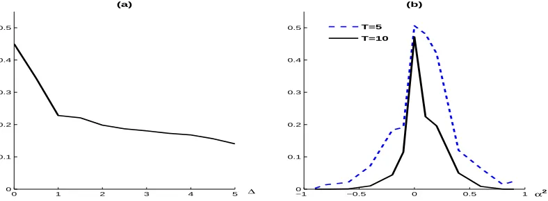
4.2 Effect of the distance between clusters

We examine two ways in which the clusters differ. First we fix the dynamics parameters both at 0.1 and vary the

equilibrium locations by takingβ1_{=0 and varyingβ}2_{. We express the normalised difference as∆ =τ}1/2_(β2_−β1_).

Figure 1(a) indicates the average probability of mis-classification, as defined above. We see that the ability to

correctly classify the data increases with the distance between the clusters, as expected. Despite the fact that the

data for both clusters have the same starting value, we already have a significant improvement in the clustering

ability when the long run levels are one (random effect) standard deviation apart.

Then we fix β1 = β2 = 0.02 andα1 = 0 and letα2 vary. Figure 1(b) shows that we can quite accurately

distinguish the clusters for α2 _{< −0.2 orα}2 _{> 0.4. In this case, we also repeat the experiment with a smaller}

time dimension,T = 5. Of course, this decreases the model performance somewhat, but we still have quite good

clustering properties for values ofα2_{far away from the extremes. In both samples, it appears to be easier to identify}

the clusters for a given|α2_|ifα2_{<0, as the implied alternating behaviour is quite noticeable.}

0 1 2 3 4 5

0 0.1 0.2 0.3 0.4 0.5

∆

(a)

−1 −0.5 0 0.5 1

0 0.1 0.2 0.3 0.4 0.5

(b)

α2

T=5 T=10

Figure 1. Average mis-classification probabilities for the simulated data. (a)α1 _=α2_{and∆is the normalised}

difference betweenβ1_andβ2_{. (b)α}1_{=0, β}1_=β2_.

5 Applications

Two real data sets are analysed in this section. The first contains per-capita GDP of European regions similar to

that used in Canova (2004) and Frühwirth-Schnatter and Kaufmann (2008). Here we focus on annual GDP growth.

The second is a panel of 738 Spanish manufacturing firms, taken from Arellano (2003, Sec. 6.7), where we model

5.1. Per-capita income of European regions 15

We use the prior in Subsections 2.1 and 2.2. The induced prior on each long-run growth level βj _{will be}

N(0.05,0.052_{) for the GDP data, and N(0,0.05}2_{) for the firms example. In the case of the GDP growth data, we}

will use a covariate, the (standardized) level of GDP in the previous period, for which the prior ofµj _{is N(0,1).}

For the correlation parametersain (18) andal in (19), we will use a uniform prior over (−1/(K−1),1) in both

applications.

MCMC samplers were run for 170,000 iterations, discarding the first 20,000 and then taking every 10th draw,

ending up with an effective size of 15,000. This required roughly 13 and 19.5 hrs on a single-core 3 GHz Xeon

processor for each application, respectively.

5.1 Per-capita income of European regions

There is a vast literature concerned with economic growth and convergence. While there seems not to be empirical

evidence of overall growth convergence (Durlauf and Johnson, 1995; Durlauf and Quah, 1999; Temple, 1999), some

clusters of homogeneous growing countries/regions or convergence clubs have been found; see e.g. Canova (2004)

and Quah (1997). Pesaran (2007), using data from the Penn World Tables, found evidence against convergence in

levels, but in favour of convergence in growth rates.

Here we concentrate on annual per-capita GDP growth rates from 258 NUTS2 European regions, for the period

1995–2004. The NUTS Classification (Nomenclature des Unités Territoriales Statistiques) was introduced by

Euro-stat in order to provide a single uniform breakdown of territorial units. NUTS2 units are of intermediate size and

roughly corresponds to regional level. These data cover 21 European countries and are collected by Eurostat, based

on the European System of National and Regional Accounts (ESA95). We define the growth of regionifrom time

t−1 to tasyi t = log(xi t/xi t−1), where xi t is the per-capita GDP of regioniat time t. Thus, we end up with a

balanced panel ofT = 9 andm = 258. As a single covariate we use the lagged level of GDP, xi t−1standardized

to have mean zero and variance one for each region. This means thatβnow corresponds to the average long-run

modal growth levels over time, whereasMcan be interpreted in terms of a stabilizing temporal effect. In particular,

for our situation with positive growth, negative values forµj _{would imply a decreasing trend of growth over time}

within cluster j.

We fit the model forK =1,2,3,4,5. Estimated log Bayes factors (BF) are shown in Table 2, a positive value

implying support in favour of the model in the row. For example, the model withK =2 is preferred over the pooled

model (K = 1) by a Bayes factor of exp(35) = 1.58×1015_{and by even more over the models withK >2. Thus,}

with unitary prior odds (or any prior odds that are likely to be used in practice), the posterior probability of the

two-cluster model will be virtually one. Interestingly, the simplest, completely pooled model is clearly preferred to

K = 3,4 and 5, but the best model by far is the one with two clusters. Since the model withK = 5 was the least

16 5.1. Per-capita income of European regions

context).

Table 2. NUTS2 GDP growth data. Log-BF, according to the number of clusters. A positive figure indicates support in favour of the model in the row.

K K

2 3 4 5

1 -35 532 2037 2295

2 567 2071 2331

3 1504 1764

4 259

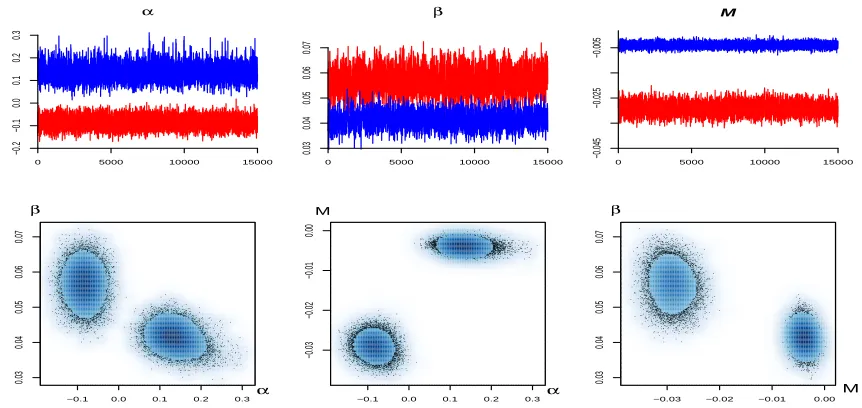
Figure 2 shows traces and scatterplots (with a smoothed density representation) of the drawn values for (α,β,M)

in the chain with two components using the permutation sampler (Frühwirth-Schnatter, 2001), to ensure we

ad-equately explore the entire posterior distribution. Both the traces and the scatterplots illustrates that the dimensions

in which the components are most different are the dynamics parameterαand the covariate effectM. Here, we use

the labelling convention according to the values ofα, and impose thatα1 _{< α}2_{in post-processing the data. This}

perfectly implements the separation between the two visually different clusters in the scatterplots. Ordering with

respect toµgives exactly the same results.

α

0 5000 10000 15000

−0.2 −0.1 0.0 0.1 0.2 0.3 β

0 5000 10000 15000

0.03 0.04 0.05 0.06 0.07 M

0 5000 10000 15000

−0.045

−0.025

−0.005

−0.1 0.0 0.1 0.2 0.3

0.03 0.04 0.05 0.06 0.07 β α

−0.1 0.0 0.1 0.2 0.3

−0.03 −0.02 −0.01 0.00 M α

−0.03 −0.02 −0.01 0.00

0.03 0.04 0.05 0.06 0.07 β M

Figure 2. NUTS2 GDP growth data. Traces and scatterplots of the sampler for α, βand M, using K = 2.

Different shades indicate cluster assignment, after post-processing.

A second important conclusion from Figure 2 is the fact that posterior dependence between the various

cluster-specific parameters is quite small. This suggests that the parameterisation used clearly distinguishes between

different aspects of the data and that the parameters have a well-defined role.

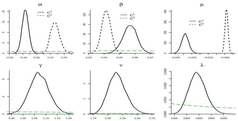
Figure 3 shows estimated marginal posterior densities for the model-specific parameters of the models with

K = 1,3,4,5. Throughout, we also plot the prior density in these graphs, indicated by long dashes. Estimation of

the common parameters is virtually unaffected by the number of clusters. Comparing the plots forαwith different

5.1. Per-capita income of European regions 17

whole panel, yielding misleading inference on the dynamics and an illusion of precise estimation (note the different

scales). Also, it is clear from the inference onαwithK = 3,4 and 5 that these models contain more clusters than

supported by the data, as there is no clear separation between the clusters with lowerαj_{. This lack of separation}

leads to markedly multimodal posteriors forµj _{and can clearly not be solved by choosing a different ordering}

constraint. It is reassuring that model choice through Bayes factors strongly avoids the inclusion of unwarranted

clusters in our model. This illustrates, in particular, the sensible calibration of our prior assumptions.

K=1

α

0.00 0.04 0.08 0.12

K=3

C1

C2

C3

−0.35 −0.10 0.15 0.40 0.65

0 3 6 9 12 15 K=4 C1 C2 C3 C4

−0.4 −0.2 0.0 0.2 0.4 0.6 0.8

0 3 6 9 K=5 C1 C2 C3 C4 C5

−0.4 −0.2 0.0 0.2 0.4 0.6 0.8

0

3

6

9

β

0.0400 0.0450 0.0500 0.0550

β

C1

C2 C3

0.02 0.03 0.04 0.05 0.06 0.07

0 20 40 60 80 C1 C2 C3 C4

0.02 0.03 0.04 0.05 0.06 0.07 0.08

0 20 40 60 80 C1 C2 C3 C4 C5

0.02 0.03 0.04 0.05 0.06 0.07 0.08

0 20 40 60 80 M

−0.010 −0.008 −0.006

0 150 300 450 C1 C2 C3

−0.04 −0.03 −0.02 −0.01 0.00

0 50 100 150 C1 C2 C3 C4

−0.05 −0.03 −0.01 0.01

0 30 60 90 120 C1 C2 C3 C4 C5

−0.05 −0.03 −0.01 0.01

0

30

60

90

Figure 3. NUTS2 GDP growth data. Prior (light long dashes) and posterior (as in legend) densities for the

cluster-specific parameters, using K =1,3,4,5. Different values of K correspond to different columns. Rows

relate to the densities ofα(top),β(middle) and M (bottom). In the legends Ci_{indicates cluster i.}

As we saw in Table 2, the two-cluster model is decisively preferred over the others. Posterior results are

displayed in Figure 4. Note that the prior onλis improper and its scaling is, therefore, arbitrary. For this best

model with two clusters, convergence is fairly rapid (values ofαj _{are not large in absolute value), and we have a}

small club of regions with small negative first order growth autocorrelation (i.e.those with a small negative value

ofα) and a larger subset with small positive first order autocorrelation, as indicated in the top left graph of Figure 4.

The posterior mean relative cluster sizes are{0.28,0.72}. In addition, Figure 5 shows the individual membership

probabilities with the regions ordered in ascending order according to initial GDP level. This illustrates that the

first cluster tends to consist of regions with relatively low GDP in 1995. In particular, it groups emerging regions

such as all of the Polish regions in the sample and most of the Czech regions, but also includese.g.Inner London

18 5.1. Per-capita income of European regions

the sequel).

α

C1

C2

−0.20 −0.10 0.00 0.10 0.20

0 4 8 12 16 β C1 C2

0.03 0.04 0.05 0.06 0.07

0 30 60 90 120 µ C1 C2

−0.035 −0.025 −0.015 −0.005

0 100 200 300 400 γ

0.95 1.00 1.05 1.10 1.15 1.20

0

4

8

ν

1.75 2.00 2.25 2.50 2.75

0

1

2

λ

1400 1600 1800 2000 2200

0.0000

0.0010

0.0020

0.0030

Figure 4.NUTS2 GDP growth data. Prior (long dashes) and posterior (as in legend) densities for parameters of

the model with K=2. For the cluster-specific parameters Ci_{indicates cluster i.}

Membership Probabilities C1 C2 Regions 0.00 0.25 0.50 0.75 1.00

Figure 5. NUTS2 GDP growth data. Membership probabilities for the model with K = 2, with the 258 units (regions) ordered according to initial GDP level. Bars indicate the posterior probability of belonging to cluster 1 for each region.

The first club has a mean value for α1 _{of -0.084, with (-0.130, -0.038) the posterior CI of probability 0.95.}

For the other club,α2_{has a mean of 0.135, and lies within (0.073, 0.208) with posterior probability of 0.95. Note}

that the posterior distribution ofαfor the pooled model (K =1) in Figure 3 is concentrated around an area which

receives only very little probability mass from the posteriors of α1 _{and α}2 _{in the two-component model, so its}

averaged nature really does not correspond to any “observed” dynamic behaviour. A summary of the marginal

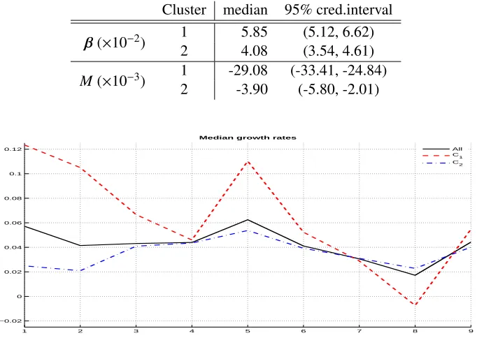
posterior distributions ofβj is shown in Table 3, which suggests that both clubs have different long-run average

growth rates. The log Savage-Dickey density ratio in favour ofβ1 _{= β}2 _{is -17.3, strongly supporting a different}

average steady-state level. The economies with alternating growth dynamics (first cluster) correspond to a higher

median growth rate of around 5.9%, while the second group has a median of about 4.1%. The lower part of Table 3

5.1. Per-capita income of European regions 19

values, implying a fairly substantial negative trend of growth over time. For the second cluster, this effect is much

smaller. Indeed, looking at Figure 6, which groups average (over regions) observed growth rates for each year, it is

clear that growth rates for cluster 1 tend to go down over the sample period, while those for cluster 2 remain almost

unaffected. It is also apparent that the time pattern of growth rates for cluster 2 is more stable, with the negative

value ofα1reflected in a more unstable growth pattern for cluster 1. This is in line with cluster 1 grouping mostly

emerging economies, which are growing more rapidly in the beginning of the sample period. Interestingly, Figure 6

suggests convergence in growth between the two clusters by the end of the sample period.

Table 3.NUTS2 GDP growth data. Summary statistics ofβandµfor the skew-t model with K=2.

Cluster median 95% cred.interval

1 5.85 (5.12, 6.62)

β(×10−2₎

2 4.08 (3.54, 4.61)

1 -29.08 (-33.41, -24.84)

M(×10−3) _{2 -3.90 (-5.80, -2.01)}

1 2 3 4 5 6 7 8 9

−0.02 0 0.02 0.04 0.06 0.08 0.1 0.12

Median growth rates

All C1 C2

Figure 6. NUTS2 GDP growth data. Median observed GDP growth over countries with membership according to maximum posterior probability. Solid line: full sample; dashed line: cluster 1; dot-dashed line: cluster 2.

Figure 4 illustrates that fat tails are a very prominent feature of these data. Posterior inference onνis quite

concentrated on small values in all cases, typicallyν∈(1.9,2.5) with 0.95 posterior probability. Also, some right

skewness is present in this data set. Indeed,γ ∈ (0.99,1.16) with posterior probability of 0.95. However, the log

Savage-Dickey density ratio in favour ofγ=1 is 1.7, providing mild evidence in favour of the symmetric model.

Given this moderate evidence in favour of γ = 1, we estimated the symmetric t model with K = 2. The

estimates of the common parameters and cluster membership probabilities (not shown) were very little affected by

imposing symmetry. We did, however, find some small differences for the cluster specific parameters, which we

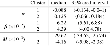
present in Table 4. Clearly, the symmetric model shifts the distribution of the long-run average levelsβto the right,

in order to compensate for the right skewness in the data. Nevertheless, all estimated medians for the parameters of

this model are contained in the corresponding 95% CI’s of the skew version and viceversa.

Frühwirth-Schnatter and Kaufmann (2008) use a related setting to model the level of per-capita income for a

20 5.1. Per-capita income of European regions

Table 4. NUTS2 GDP growth data. Summary statistics of the cluster-specific parameters, using the symmetric

t-model with K =2.

Cluster median 95% cred.interval

1 -0.088 (-0.134, -0.041)

α _{2 0.125 (0.066, 0.184)}

1 6.22 (5.61, 6.88)

β(×10−2₎

2 4.39 (4.00 4.78)

1 -29.62 (-33.62, -25.74)

M(×10−3₎

2 -4.16 (-5.98, -2.38)

time point, by the European average (see Canova, 2004). This effectively reduces the dynamic behaviour of the

individual regions to movement within the European distribution of incomes. In addition, this data set differs from

our growth data in that it does not include any Central European regions (or regions in Finland, Sweden and Latvia).

Bearing this in mind, we analysed this data set chiefly for comparison with their results. We fitted our model to

these level data, usingK = 2 and no covariates. Like Frühwirth-Schnatter and Kaufmann (2008), we found two

well separated clusters, summarized in Table 5, with estimated relative sizesη= (0.13,0.87)0_{. Thus, we have one}

small converged cluster withα1_{close to zero and a large group with important dynamic behaviour whereα}2_{is very}

close to one. Despite the large differences in dynamic behaviour, there is no overwhelming difference in long-term

levels (as measured byβ).

Table 5. NUTS2 income level data. Summary statistics of the cluster-specific parameters using both t models

with K=2. Numbers reported are median (95% CI).

Clus Skew-t t

1 0.014 (-0.020, 0.045) 0.017 (-0.014, 0.049)

α _{2 0.993 (0.988, 0.998) 0.992 (0.988, 0.996)}

1 -0.038 (-0.129, 0.057) -0.086 (-0.184, 0.041)

β _{2 0.023 (-0.070, 0.112) -0.102 (-0.190, -0.007)}

Clustering regions according to maximum posterior probabilities, yields m₁ = 15 and m₂= 129, not unlike

the results in Frühwirth-Schnatter and Kaufmann (2008). However, our membership assignments are not quite the

same as those in Frühwirth-Schnatter and Kaufmann (2008). We have to keep in mind, though, that their model

uses initial income as a covariate for the membership probability.

Our model here differs from the one used in Frühwirth-Schnatter and Kaufmann (2008) in a number of respects,

the following of which can have most effect on the results in this application:

i. We do not allow for unit roots, which is of some importance here as thear(1) process on the levels is close

to a unit root for one of the two clusters they find (see their Table 5 and our Table 5). Note that with these

data we are modelling levels rather than growth rates.

ii. The other priors are also quite different. They use normals throughout, centred at 0 and with higher variances

5.2. Spanish firm employment 21

iii. They do not allow for skewness. Left skewness, however, is a prominent feature of the data, as γ ∈

(0.815,0.892) with prob. 0.95. As we have seen with both the simulated and the growth data, neglecting

skewness can have an important impact on the estimation of the steady-state levels.

iv. They fix the degrees of freedom for the Student-tmodel at 8. In contrast, we find the tails to be extremely fat,

with (1.1,1.3) the 95% CI forν, irrespective of the model used (skewed or symmetric). Of course, this will

also affect the estimated observational variance and can well influence the clustering (see Subsection 4.1).

In line with the latter point, the evidence in favour of Student-ttails over normal tails is overwhelming, both for

symmetric and skewed models. Once we choose a Student model, skewness is strongly preferred by the data. For

normal models, however, the log Savage-Dickey density ratio in favour ofγ =1 is 3.12 (which is in line with the

BF obtained from the bridge sampler). It is quite unusual to see the evidence in favour of skewness disappear when

we ignore the heavy tails. Thus, if we would not consider (unknown) heavy tails, we would be led dramatically

astray in the evidence regarding skewness. Of course, all other models are massively dominated by the skew-t

model. Table 5 presents the estimated cluster-specific parameters for both skewed and symmetrictmodels. The

effect of neglecting skewness is similar to that with the previous data: while the dynamics are not much influenced

by the inclusion of skewness, long-run levels are affected (but due to the left skewness, now in the other direction).

Note thatβ2_{is shifted much more thanβ}1_.

5.2 Spanish firm employment

The data set is described in the Appendix of Alonso-Borrego and Arellano (1999) and is also used in Arellano

(2003, Sec. 6.7). It consists of a balanced panel of 738 manufacturing companies, recorded yearly from 1983 to

1990 and represents more than 40% of the Spanish value added in manufacturing in 1985.

In particular, we model employment growth in these firms. With our model described in Section 2, and letting

K = 1, we obtain 95% CI’s of (0.04, 0.08) for αand (-0.0043, 0.0030) forβ. Again, inference on parameters

common to models with different values ofKis virtually unaffected by the choice of the number of clusters.

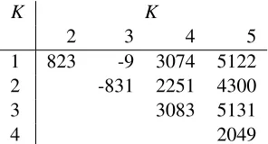
As shown in Table 6,K = 1 is strongly preferred toK = 2,K = 4 andK = 5. However, the model with three

clusters performs considerably better than the pooled model, and we will concentrate on the model withK = 3 in

the sequel. Since the model with five clusters was not preferred to any other, we did not use larger values ofK.

Table 6. Spanish firm data. Log-BF, according to the number of clusters. A positive figure indicates support in favour of the model in the row.

K K

2 3 4 5

1 823 -9 3074 5122

2 -831 2251 4300

3 3083 5131

22 5.2. Spanish firm employment

Scatterplots of the drawn values for (α,β) in the chain withK = 3 clearly suggest that identifying the labels

through ordering the values ofαj_{is the natural approach, just like in the previous example.}

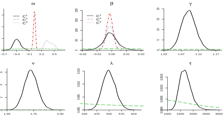
From the posterior densities in Figure 7, it is apparent that tail behaviour is extremely heavy and very well

determined by this (fairly large) data set. These data also clearly present right skewness with (1.05, 1.13) the 95%

CI forγ. Both the Savage-Dickey density ratio and bridge sampling indicate massive evidence in favour of the

skewed model.

α

C1

C2

C3

−0.7 −0.4 −0.1 0.2 0.5

0 5 10 15 β C1 C2 C3

−0.02 −0.01 0.00 0.01 0.02

0 50 100 150 200 γ

1.02 1.07 1.12 1.17

0 5 10 15 20 ν

1.50 1.75 2.00

0

2

4

6

λ

420 470 520 570 620

0.000

0.005

0.010

0.015

τ

1000 1500 2000 2500 3000

0.0000

0.0005

0.0010

0.0015

Figure 7. Spanish firm data. Prior (long dashes) and posterior (as in legend) densities for parameters of the

model with K=3. For the cluster-specific parameters Ci_{indicates cluster i.}

The relative size of each cluster, i.e.the average probability of cluster membership, is {0.132,0.651,0.217}.

From Figure 7 is is obvious that there are two relatively small clusters of “extreme” dynamic behaviour: one with

negativeα(suggesting alternating behaviour) and one with positiveα(slowly converging) existing besides one big

club with more or less random walk employment behaviour. In fact, the cluster displaying negative αtends to

contain smaller firms, which are more volatile and often overadapt to market situations. Firms that have a high

probability of belonging to the slowly converging cluster are typically larger firms which display much more stable

long-term employment strategies. The firms in the main cluster cover a wide range of sizes and have, on average,

experienced a small decline in employment over the sample period. Again, the effect of pooling all units to estimate

the dynamics parameter is apparent from comparing Figure 7 with the 95% CI of (0.04, 0.08) forαwithK = 1:

rather than gaining strength in the process, opposites are averaged out and the spread of the dynamic behaviour is

dramatically underestimated when we use only one cluster.

We have already reported that the skewed model is strongly favoured by the data over its symmetric counterpart.

In order to assess whether allowing for skewness makes a practical difference in this example, we have estimated

the symmetric Student model (i.e.γ = 1) with 3 components. The main difference is in the equilibrium values

βj. The posterior medians forβj with skewness were all within (-0.0011, -0.0008), and these are now all positive,

5.2. Spanish firm employment 23

account the skewness, we would erroneously conclude that long-run employment growth is positive, whereas our

skewed model assigns most probability to negative equilibrium growth of employment in Spanish manufacturing

firms.

Both for the skewed and symmetric cases, the three clusters of firms converge to very similar equilibrium levels,

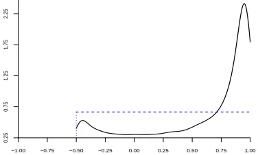
suggesting that we might also pool this parameter to gain strength. Figure 8 shows that the posterior density of the

correlation parametera, as defined in (18), has a lot of mass close to one and thus strongly supports this model

simplification. This is confirmed by the formal log-BF in favour of commonβj_{’s, which is estimated at 13.4. Other}

parameters are virtually unaffected by this reduction of the model. The common long-run levelβ∈(−0.005,0.003)

with posterior probability 0.95, very much in line with the results for cluster-specificβj_{’s with the skew-tmodel}

(see Figure 7), except that inference is now a bit more precise as a consequence of borrowing strength.

−1.00 −0.75 −0.50 −0.25 0.00 0.25 0.50 0.75 1.00

0.25

0.75

1.25

1.75

2.25

Figure 8. Spanish firm data. Posterior (solid) and prior (dashed) densities for a in(18)using K =3. Note that

a∈(−1/(K−1),1).

Finally, we calculate the predictive distribution of the employment of two firms in the sample for 1991 (one

year after the last observation in the sample), using a commonβ. As we are predicting employment itself (rather

than its growth), we condition on the actual employment values in the sample years. Firms 433 and 31 are selected:

the former grows from 30 to 37 employees in 1990 and in the model withK=3 it is assigned to the three clusters

with posterior weights {0.834,0.165,0.001}; the latter shrinks its employment in 1990 from 126 to 62 and has

cluster probabilities{0.324,0.636,0.040}. Figure 9 presents these predictives for the pooled model (K=1) and the

model with three components (a symmetric and a skewed version). The model withK = 1 has a slightly positive

αand will thus concentrate the predictive at a value which slightly extends the last observed movement. In the

three-cluster model, Firm 433 (Figure 9 (a)) has most mass on the first cluster, which corresponds to large negative

values forα(see Figure 7), and will thus counteract the last movement, which results in much more predictive mass

on lower employment values. Firm 31 has non-negligible mass for all three clusters and this results in a multimodal

predictive, with the first cluster providing predictive mass around 80 (partially counteracting the last movement)

and the third (least important) cluster resulting in slightly more weight on lower values. The latter is a consequence

of the large positive values for the dynamics parameters, which lead to a pronounced extrapolation of the last

observed change. Finally, the second cluster (which has most of the weight) corresponds to very small, mostly