Synaptic shot noise and conductance fluctuations affect the membrane voltage with equal significance

University of Warwick institutional repository: http://go.warwick.ac.uk/wrap

This paper is made available online in accordance with

publisher policies. Please scroll down to view the document

itself. Please refer to the repository record for this item and our

policy information available from the repository home page for

further information.

To see the final version of this paper please visit the publisher’s website.

Access to the published version may require a subscription.

Author(s): Magnus J. E. Richardson and Wulfram Gerstner

Article Title: Synaptic Shot Noise and Conductance Fluctuations Affect

the Membrane Voltage with Equal Significance

Year of publication: 2005

Link to published article: http://dx.doi.org/10.1162/0899766053429444

Publisher statement: © MIT Press 2005. M. J. E. Richardson

and W. Gerstner. 2005. Synaptic Shot Noise and

Synaptic Shot Noise and Conductance Fluctuations Affect the

Membrane Voltage with Equal Significance

Magnus J. E. Richardson

magnus.richardson@epfl.ch

Wulfram Gerstner

wulfram.gerstner@epfl.ch

Laboratory of Computational Neuroscience, I&C and Brain-Mind Institute, Ecole Polytechnique F´ed´erale de Lausanne, CH-1015 Lausanne EPFL, Switzerland

The subthreshold membrane voltage of a neuron in active cortical tissue is a fluctuating quantity with a distribution that reflects the firing statistics of the presynaptic population. It was recently found that conductance-based synaptic drive can lead to distributions with a significant skew. Here it is demonstrated that the underlying shot noise caused by Poisso-nian spike arrival also skews the membrane distribution, but in the op-posite sense. Using a perturbative method, we analyze the effects of shot noise on the distribution of synaptic conductances and calculate the con-sequent voltage distribution. To first order in the perturbation theory, the voltage distribution is a gaussian modulated by a prefactor that captures the skew. The gaussian component is identical to distributions derived using current-based models with an effective membrane time constant. The well-known effective-time-constant approximation can therefore be identified as the leading-order solution to the full conductance-based model. The higher-order modulatory prefactor containing the skew com-prises terms due to both shot noise and conductance fluctuations. The diffusion approximation misses these shot-noise effects implying that analytical approaches such as the Fokker-Planck equation or simulation with filtered white noise cannot be used to improve on the gaussian ap-proximation. It is further demonstrated that quantities used for fitting theory to experiment, such as the voltage mean and variance, are robust against these non-Gaussian effects. The effective-time-constant approxi-mation is therefore relevant to experiment and provides a simple analytic base on which other pertinent biological details may be added.

1 Introduction

Given a perfect model of the membrane response to synaptic input, it would be possible to infer from the distribution of the subthreshold, membrane-voltage fluctuations many quantities of interest, such as the levels of activity and correlations in the excitatory and inhibitory presynaptic populations.

Early models of synaptic input (Stein, 1965) comprised a leaky integrator driven by a stochastic current, which generated postsynaptic potentials of fixed amplitude. Since then, great effort has been made to incorporate fur-ther biological details.

Soon after the publication of Stein’s model, synaptic conductance ef-fects began to be addressed (Stein, 1967; Johannesma, 1968; Tuckwell, 1979; Wilbur & Rinzel, 1983; Lansky & Lanska, 1987). These early models fea-tured unfiltered, delta-pulse synapses and were primarily concerned with the statistics of the interspike interval distribution. Although the majority of studies used the diffusion approximation (i.e., the limit of high synaptic rates and low postsynaptic potential amplitudes), the effects of shot noise due to Poisson distributed pulse arrival at low rates have also been consid-ered (see, e.g., Tuckwell, 1989) in the context of stochastic resonance (Hohn & Burkitt, 2001) and the neural response to correlations in the presynap-tic population (Kuhn, Aertsen, & Rotter, 2003). Other studies have exam-ined the filtering of the incoming pulses at the synapses and have shown it can lead to unexpected dynamical response properties: synaptic filtering can, paradoxically, allow neurons to follow high-frequency signals better (Brunel, Chance, Fourcaud, & Abbott, 2001; Fourcaud & Brunel, 2002).

More recently, a number of experimental studies have directly mea-sured the effect of synaptic drive on the membrane voltage (Kamondi, Acsady, Wang, & Buzsaki, 1998; Destexhe & Par´e, 1999; Sanchez-Vives & McCormick, 2000; Monier, Chavane, Baudot, Graham, & Fr´egnac, 2003; Holmgren, Harkany, Svennenfors, & Zilberter, 2003). The availability of such measurements has led to a renewed interest in the quantitative modeling of synaptic drive, with a view to infer presynaptic network states from voltage fluctuations (Stroeve & Gielen, 2001; Rudolph, Piwkowska, Badoual, Bal, & Destexhe, 2004), compare current and conductance-based models of synap-tic drive (Tiesinga, Jos´e, & Sejnowski, 2000; Rauch, La Camera, L ¨uscher, Senn, & Fusi, 2003; Rudolph & Destexhe, 2003; Jolivet, Lewis, & Gerstner, 2004; Richardson, 2004; La Camera, Senn, & Fusi, 2004; Meffin, Burkitt, & Grayden, 2004), and explore mechanisms for the gain control of the neuronal response (Chance, Abbott, & Reyes, 2002; Burkitt, Meffin, & Grayden, 2003; Destexhe, Rudolph, & Par´e, 2003; Fellous, Rudolph, Destexhe, & Sejnowski, 2003; Prescott & De Koninck, 2003; Grande, Kinney, Miracle, & Spain, 2004; Kuhn, Aertsen, & Rotter, 2004).

2 Membrane Response to Synaptic Drive

In this section, the full model of the membrane response to synaptic drive is introduced and two common approximations to this model outlined. An analysis of the aspects of the drive missed by these approximation schemes will motivate the development of a perturbative approach.

2.1 The Full Model. Following Stein (1967), the membrane voltageV(t) responds passively to synaptic drive: voltage gated channels, including spike-generating currents, are not included. The membrane is modeled by a capacitanceCin parallel with a leak conductancegLand two fluctuating

excitatoryge(t) and inhibitorygi(t) conductances with equilibrium

poten-tials atEL,Ee, andEi, respectively. This system therefore comprises three

independent variables:

Cd V

dt = −gL(V−EL)−ge(V−Ee)−gi(V−Ei)+Ia pp (2.1)

τe dge

dt = −ge+ceτe

{tke} δt−tke

(2.2)

τi dgi

dt = −gi+ciτi

{tki} δt−tki

. (2.3)

The excitatory conductance is driven by pulses that arrive at the Poisson-distributed times {tke} at a total rate Re summed over all input fibers.

Each pulse provokes a quantal conductance increase ce, which then

de-cays exponentially with a time constantτe. The inhibitory conductance is

defined analogously. Any experimentally applied current is accounted for byIa pp.

In this letter, only the steady-state statistical properties will be considered. Thus, all expectations of a quantityx(t), written asx(t), denote either an average over an ensemble of statistically independent systems, in which any transients due to initial conditions are no longer present, or the temporal average ofx(t) in a single system.

2.2 The Diffusion Approximation. For the case in which the rates Re,Ri are relatively high, the number of pulses that arrive within the

timescalesτe, τi will be approximately gaussian distributed. The

replace-ment of the synaptic shot noise in equations 2.2 and 2.3 by a constant term and gaussian white noise constitutes the diffusion approximation. Thus, using excitation as an example,

τe dge

dt ge0−ge+

√

where the gaussian white noiseξe(t) has a mean and autocorrelation function

defined by

ξe(t) =0 ξe(t)ξe(t) =τeδ(t−t). (2.5)

The Ornstein-Uhlenbeck process (see equation 2.4) has been shown to cap-ture the statistics of conductance fluctuations at the soma of compartmental-ized model neurons (Destexhe, Rudolph, Fellous, & Sejnowski, 2001). The average conductancege0 and the standard deviationσe are related to the

variablesce, τe, andRethrough

ge0=ceτeRe, σe=ce

τeRe

2 . (2.6)

By construction, the first two moments of the diffusion approximation are identical to those of the shot noise process. Higher moments, however, are not correctly reproduced in the diffusion approximation.

The conductance equation 2.4 is linear and can be integrated.1_The

fluc-tuating componentge Fof the conductance is

ge F(t)≡ge(t)−ge0 √

2σe

_∞

0 ds

τe e−s/τe ξ

e(t−s), (2.7)

which yields (with equation 2.5) the gaussian distribution

pD(ge)=

1

2πσ2 e

exp

−(ge−ge0)2

2σ2 e

. (2.8)

The subscript signifies that the calculation was made in the diffusion ap-proximation. There are clearly some problems with distribution 2.8 if the conductance meange0is of a similar magnitude to the standard deviationσe.

In this regime, the diffusion approximation predicts negative conductances (Lansky & Lanska, 1987; Rudolph & Destexhe, 2003). In fact, the criterion for validity of the diffusion approximation is

σe/ge01, (2.9)

suggesting that this approximation misses higher-order terms scaling with powers ofσe/ge0. Thus, the shot noise conductance fluctuations should read

ge F(t)= √

2σe

_∞

0 ds

τe e−s/τe

ξe(t−s)+corrections∝ σe ge0

, (2.10)

whereξe(t) is the gaussian white noise defined in equation 2.5.

2.3 The Diffusion Approximation Is Inconsistent. The combination of the diffusion approximation of the synaptic drive (see equation 2.4 and its equivalent for inhibition) and the full voltage equation, 2.1, will now be examined. By separating the synaptic conductances into tonic components

ge0,gi0and fluctuating components ge F,gi F, the voltage equation can be

written as

Cd V

dt = −g0(V−E0)−ge F(V−Ee)−gi F(V−Ei), (2.11)

where the total conductanceg0and drive-dependent equilibrium potential E0are defined by

g0=gL+ge0+gi0 and E0=

1

g0

(gLEL+ge0Ee+gi0Ei+Ia pp).

(2.12)

The subscripts 0 anticipate that these quantities are correct at the zero order of a perturbation expansion that will be developed in a later section. The total conductanceg0 suggests the introduction of an effective membrane

time constant,

τ0=C/g0. (2.13)

This feature of the synaptic drive was identified in the early analytic treat-ment of Johannesma (1968).

The fluctuation terms driving the voltage in equation 2.11 will now be examined. Taking excitation as an example, the voltage-dependent compo-nent of the drive can be expanded around the equilibrium potentialE0,

ge F(V−Ee)=ge F(E0−Ee)+ge F(V−E0). (2.14)

seen that this term represents fluctuations ing0, or equivalently inτ0, the

effective membrane time constant.

These two noise terms are, however, not equally significant. The quan-tity V−E0 grows (linearly) with the fluctuationsge F,gi F. So whereas the

additive noise terms are of the orderge F,gi F, the multiplicative noise terms

are of the orderg2

e F,g2i F, andge Fgi F. This suggests that (1) the multiplicative

noise terms could be neglected if the noise strength was in some way small, and (2) if these terms were retained, the effects of the synaptic drive on the membrane voltage would be modeled in greater detail. Point 1 is valid, as will be seen in section 2.4. Point 2, however, is false due to an unexpected weakness of the diffusion approach with multiplicative noise. This will now be outlined.

On reexamining equations 2.7 to 2.9, it is seen that relative to the tonic con-ductance, the fluctuations in the diffusion approximation scale withσe/ge0.

But equation 2.10 states that the terms missed by this approximation scale with the square of this quantity. Hence,

ge F/ge0=A

σe ge0

+B

σe ge0

2

+ · · · (2.15)

where Ais the diffusion-level term andBis the first-order correction due to shot noise. Given that σe/ge0 is the small quantity parameterizing the

diffusion approximation, it is clearly inconsistent to neglect the second-order termB in the additive noisege F(Ee−E0) of equation 2.14 but keep

the implicit A2 _{term in the multiplicative noiseg}

e F(V−E0)∝g2e F. This is,

however, what occurs in the diffusion approximation.

This result is surprising because it implies that although diffusion-based approaches (such as the Fokker-Planck equation or any simulation with filtered gaussian noise) purport to capture the effects of synaptic-conductance fluctuations, they miss equally important terms due to the shot noise. However, it should be stressed that almost all previous studies of conductance-based synaptic noise that used the diffusion approximation implicitly concentrated their analyses on the dominant effects coming from the tonic conductance increase and additive noise term; the conclusions of such studies remain valid.

2.4 The Effective-Time Constant Approximation. This is also known as thegaussian approximationof the voltage distribution. The treatment of the membrane voltage can easily be made consistent with the diffusion approximation of the synaptic conductance equations. This is achieved by dropping the multiplicative noise term, that is, by neglecting conductance fluctuations, to yield

Cd V

This voltage equation is of the form of a current-based model, but the dom-inant effect of the synaptic conductance is accounted for through the use of an increased effective leakg0. This approximation is in widespread use,

having been applied to white noise synaptic drive (Wan & Tuckwell, 1979; Lansky & Lanska, 1987; Burkitt & Clark, 1999; Burkitt, 2001; Burkitt et al., 2003, La Camera et al., 2004), alpha-pulse synapses (Manwani & Koch, 1999), and, more recently (Richardson, 2004), to the case of exponentially filtered synapses studied here. The equation set comprising the voltage equation 2.16 and the diffusion approximations for the conductances are simple to analyze and can be integrated to give

V(t)−E0 √

2

σe g0

(Ee−E0)

(τe−τ0)

_∞

0

dse−s/τe−_e−s/τ0ξ e(t−s)

+√2

σi g0

(Ei−E0)

(τi−τ0)

_∞

0

dse−s/τi−_e−s/τ0ξ i(t−s).

(2.17)

This equation has an obvious interpretation: the quantities multiplying the noise are just the excitatory and inhibitory postsynaptic potentials for a membrane with an effective time constantτ0. The fact that it is linear in

the noise means that many quantities of interest can be easily calculated, including temporal measures such as the autocorrelation function.

The distribution predicted for the voltage is the gaussian

p0(V)=

1

2πσ2 V

exp

−(V−E0)2

2σ_V2

, (2.18)

where, for the case where there are no correlations between excitation and inhibition, the variance is (Richardson, 2004)

σ2 V=

σe g0

2

(Ee−E0)2 τe

(τe+τ0) +

σi g0

2

(Ei−E0)2 τi

(τi+τ0)

. (2.19)

If the limit τe, τi→0 is correctly taken (by keeping the quantities ceτe/C

andciτi/C fixed), it can be shown that this variance is compatible with

made to yield results that correspond, at the gaussian level and in the steady state, to the distribution parameterized by equations 2.12 and 2.19.

2.5 The Aim of This Letter. The gaussian approximation provides a mathematically convenient approach to the analysis of conductance-based synaptic drive and is accurate for parameter values relevant to experiment (Richardson, 2004). Given the analysis presented above, it is clear that to improve on the gaussian approximation, both shot noise and conductance fluctuations must be included. The goal of the next two sections will be to de-velop a perturbative method that allows for the consistent calculation of the conductance and voltage distributions at a higher order than the gaussian approximation. These higher-order calculations will yield the skew of the voltage distribution, a quantity that is measurable experimentally. More important, the approach will provide information on the validity of fitting gaussian-level analytical forms for the mean and variance to voltage traces of cortical neurons. To aid readability, only the results of the calculations are given in the main body of the article. However, the methods developed here are applicable to other areas of theoretical neuroscience, such as the distribution of amplitudes at depressing synapses (Hahnloser, 2003) or the shape of synaptic weight distributions (van Rossum, Bi, & Turrigiano, 2000; Rubin, Lee, & Sompolinsky, 2001), and are therefore presented in full in the appendixes.

3 Synaptic Shot Noise and Conductance Distributions

In this section, the effects of shot noise on the synaptic conductance distri-butions will be analyzed. It should be noted that relaxation processes with shot noise, for which equations 2.2 and 2.3 are examples, have been well studied, and an exact solution (Gilbert & Pollak, 1960) for the distribution, in the form of a recursion relation, does exist. However, the aim of the approach (in section 4) is to incorporate the shot-noise conductance fluctuations into a model of the membrane voltage. A perturbative approach is better suited to this purpose. For this reason, the full solution for the shot-noise distribu-tion pS(ge) will not be presented here but, when needed, will be obtained

by numerical simulation of equation 2.2.

3.1 The Diffusion Approximation Misses the Skew. In the limit where the standard deviation σe has a similar magnitude to the conductance

meange0, the diffusion approximation, unlike the full model, predicts

-1 0 1 2 3 4

Conductance g

/ c

0.00 0.02 0.04 0.06 0.08 0.10 0.12

Difference

| p_D - p_S | | p_P - p_S |

-1 0 1 2 3 4

Conductance g

/ c

0 0.1 0.2 0.3 0.4 0.5 0.6 0.7

Distribution

shot noise p_S diff. approx. p_D perturb. theory p_P

-1 0 1 2 3 4 5 6 7

Conductance g

/ c

0 0.1 0.2 0.3 0.4 0.5

-1 0 1 2 3 4 5 6 7

Conductance g

/ c

0.00 0.01 0.02 0.03 0.04 0.05 0.06

A C

B D

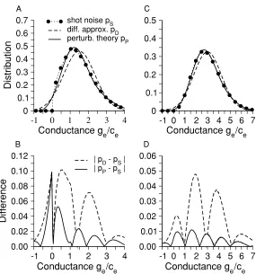
Figure 1: Distribution of shot noise conductance fluctuations; the perturbation theory improves on the diffusion approximation. (A) Comparison of the full distributionpSgenerated by the simulation of equation 2.2 to the diffusion ap-proximationpD(see equation 2.8) and the perturbation theorypP(see equation 3.4) for the caseσe/ge0=0.60 (Reτe =1.5). (B) The corresponding absolute differ-ence between the diffusion approximation and full solution|pD−pS|and also the perturbatively generated distribution and the full solution|pP−pS|. The perturbative distribution reduces the error caused by both the negative con-ductances and the skew. (C, D) Analogous measures for the caseσe/ge0=0.41 (Reτe =3.0) for which the theoretical approaches can be expected to be more accurate. Details of the simulations are given in appendix A.

comparison can be made between the full and approximate distributions shown in Figure 1A. In this case (for whichReτe=1.5 implyingσe/ge0=

0.60), the peak of the shot noise distribution is to the left of that of the gaussian. Because both distributions have the same mean conductance

a longer tail to the right. Any improvement of the diffusion approximation should address both the negative conductivity and the skew of the conduc-tance distribution.

3.2 Accounting for the Shot Noise. The corrections identified in equation 2.10 will now be accounted for. A stochastic variable ζe(t),

analogous to gaussian white noiseξe(t),

τe dge

dt ge0−ge+

√

2σe ζe(t), (3.1)

can be constructed that has statistics that capture the shot noise fluctuations correctly up to the next order missed by the diffusion approximation. It can be shown that such a quantity must obey the same first- and second-order correlators as gaussian white noise,

ζe(t) =0, ζe(t)ζe(t) =τeδ(t−t), (3.2)

but also a new third-order correlator,

ζe(t)ζe(t)ζe(t) = √

2

σe ge0

τ2

eδ(t−t)δ(t−t). (3.3)

It is this third-order correlator, proportional to σe/ge0, that provides the

leading-order correction to the diffusion approximation. All higher-order correlators of products of ζe(t) factorize in terms of these first-, second-,

and third-order correlators. Using the rules in equations 3.2 and 3.3, the conductance distribution can be shown (see appendix B) to be

pP(he)=

1 √

2π

1+ 4 3

σe ge0

h3 e

3! −

he

2!

exp

−h2e

2

, (3.4)

wherehe =(ge−ge0)/σeis the normalized conductance and the subscriptP

denotes that the result was derived as a perturbative expansion in the small variablesσe/ge0. The distribution takes the form of a gaussian modulated

by a prefactor. To zero order inσe/ge0, the prefactor is equal to one, and

the gaussian distribution 2.8 is recovered. The prefactor terms proportional toσe/ge0now allow for the moments of the distribution to be calculated at

higher order. The mean and variance are unchanged, as would be expected given the previous comments about the exactness of these two moments. The first new result of the perturbation theory is the skewSgeof the

distri-bution:

Sge=

1

σ3 e

(ge−ge0)3

=h3_e=4

3

σe ge0

A useful aspect of the perturbation theory is that this skew is exact. The distribution itself and its higher moments are, however, correct only at the given order of the series expansion inσe/ge0. Two examples comparing the

numerically generated conductance distribution pS, diffusion

approxima-tionpDand perturbation theorypP, are plotted in Figure 1.

4 The Subthreshold Voltage Distribution

The model of synaptic conductance studied in the previous section can now be incorporated into the membrane voltage equation. This will allow the voltage distribution to be calculated at the next order beyond the gaussian approximation. The method involves a perturbative solution to the voltage equation 2.1, the excitatory synaptic conductance equation 3.1, and its in-hibitory analog. For the perturbative calculation of the voltage distribution, it is convenient to use the following small parameters,

xe=σe/g0 and xi=σi/g0, (4.1)

which are linearly related (inσe, σi) to the small parameters of the

conduc-tance expansionσe/ge0andσi/gi0. The calculation for the voltage

distribu-tion is given in appendix C and, in terms ofv=V−E0, can be written in

the form

pP(v)=

1

2πσ2 V

1+ v

σV

µV σV

− S 2!

+ v3

σ3 V

S 3!

exp

− v2 2σ2

V

, (4.2)

where the subscriptPdenotes the perturbatively generated result. The volt-age appears only through the ratiov/σV, and the other termsµV/σVandS

are parameters proportional toxe,xi: this distribution generates moments vm_/σm

V that are correct up to orderxe,xi.

The quantityµVis the leading-order correction to the voltage meanE0

and stems from the conductance fluctuations only: the shot noise does not influence the mean voltage. The standard deviation, given by equation 2.19, is identical to the gaussian valueσVand is therefore unaffected by shot noise

or multiplicative conductance at this order in the perturbation expansion. Thus,

V −E0=µV and (V− V)2 =σV2. (4.3)

The third-order moment of the distribution 4.2 gives the skew of the voltage distribution,

1

σ3 V

From the expression given in appendix C, equation C.20, it can be seen that two distinct contributions to the skew naturally arise: one from the shot noiseSSNand a second one from the conductances fluctuationsSC F. These

two contributions to the skew are equally significant because they are both proportional toxe,xi. This illustrates one of the central points of this study:

the diffusion approximation of a conductance-based model with multiplica-tive noise is inconsistent because it misses the shot noise contributionSSN.

The full set of equations forµV,σV, andSis given in appendix D.

4.1 An Example with Relevance to Experiment. To illustrate the ef-fects of shot noise and conductance fluctuations, a scenario is considered in which the fluctuations due to the inhibitory component of the drive can be neglected. There are two different situations that allow this action to be taken. The first is when inhibition is absent. The second, and more interest-ing, case is relevant to experiments designed to isolate the effect of excitation on the membrane voltage (Silberberg, Wu, & Markram, 2004). In such ex-periments, the neuron is hyperpolarized through the injection of current so that the mean voltageE0is near the reversal of inhibitionEi. In such cases,

the factorEi−E0multiplying all inhibitory contributions to membrane

fluc-tuations is relatively small, and such contributions can be dropped without significant loss of accuracy. Inhibition enters only through an increase of the tonic conductanceg0and the corresponding decrease of the effective time

constantτ0.

For either of these scenarios, the moments that parameterize the distri-bution in equation 4.2 take the values

µV = −xe2(Ee−E0) τe

(τe+τ0)

(4.5)

σ2

V =xe2(Ee−E0)2 τe

(τe+τ0)

(4.6)

SSN=xe

8 3

g0 ge0

(τe+τ0)2

(τe+2τ0)(2τe+τ0)

_τ

e

(τe+τ0)

(4.7)

SC F = −4xe

3τ2

e +6τeτ0+2τ02

(τe+2τ0)(2τe+τ0)

_τ

e

(τe+τ0).

(4.8)

Equations 4.7 and 4.8 give the positive and negative contributions to the skew (see equation 4.4) that come from the shot noise and conductance fluctuations, respectively.

For the case of purely excitatory drive,g0=gL+ge0, the relative

impor-tance of these contributions can be gauged by examining the ratio

SSN

SC F = 2

3

τL

(τL−τ0)

(τe+τ0)2

3(τe+τ0)2−τ02

-0.02 0 0.02 0.04 0.06 Conductance g_e (mS/cm2)

0 10 20 30 40 50 60 70 80 Distribution diff. approx. perturb. theory shot-noise sim.

-75 -70 -65 -60 -55 -50 -45 Voltage V (mV) 0.00 0.02 0.04 0.06 0.08 0.10

0.12 ETC approx. perturb. theory full model sim.

Low-conductance state: g₀=0.0667mS/cm2, τ

0=15ms

0 0.05 0.1 0.15 0.2 x_e=σ_e/g₀ -0.4 -0.2 0.0 0.2 0.4 Skew

-0.1 0 0.1 0.2 0.3 0.4 Conductance g_e (mS/cm2)

0 1 2 3 4 5 6 7 Distribution

-120 -100 -80 -60 -40 -20 Voltage V (mV) 0.00

0.01 0.02 0.03 0.04

High-conductance state: g₀=0.2mS/cm2, τ₀=5ms.

0 0.1 0.2 0.3 0.4 x_e=σ_e/g₀ -1.2 -0.8 -0.4 0.0 0.4 Skew

A B C

D E F

S_SN

S_CF

S_SN

S_CF S_SN+ S_CF

S_SN+ S_CF

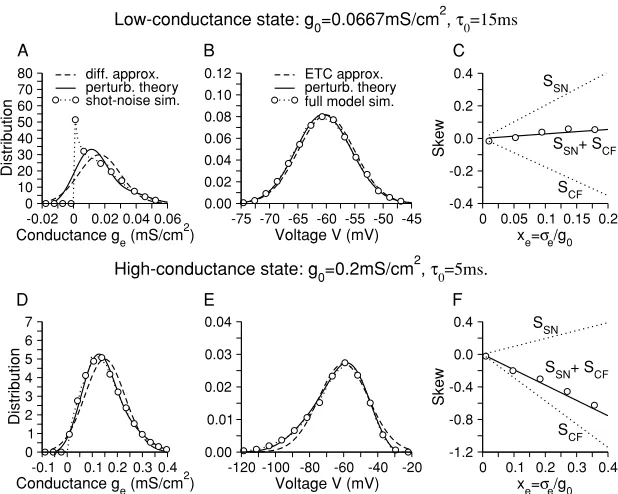
Figure 2: Distribution of the membrane voltage; perturbation theory captures the skew. A neuron is subject to a purely excitatory synaptic drive with a current

Iappapplied such thatE0= −60 mV. (A, B) The conductance and voltage dis-tributions for a low conductance state (ge0=0.0167, gL=0.05 mS/cm2) with noise strengthxe =σe/g0=0.2. The perturbative conductance distribution (see equation 3.4) is not accurate becauseσe/ge0=0.8. The weak skew of the corre-sponding voltage distribution (B) is, however, correctly predicted by the per-turbation theory (see equation 4.2) because the underlying conductance skew is exact. (C) The voltage skew (see equations 4.7 and 4.8) is plotted as a function of

xefor the same parameters, but with increasing noiseσe. The shot noiseSSNand conductance-fluctuationSC F contributions to the skew nearly cancel, explain-ing the almost gaussian voltage distribution inB. (D, E) A high conductance state (ge0=0.15 mS/cm2) withxe =σe/g0=0.4. (E) The large skew of the volt-age distribution is captured by the perturbation theory. (F) The voltvolt-age skew is negative for the high-conductance case becauseSC F dominates. Details of the simulations are given in appendix A.

whereτL=C/gL is the leak time constant. The ratio is a monotonically

increasing function of the effective time constantτ0. In the limit of low

con-ductance states, for whichτ0→τL, the ratio diverges, and the contribution

results underline the fact that the effect of shot noise is nonnegligible: even in extremely high conductance states it still comprises just under a third, SSN/S=2/7, of the net skew. These results are illustrated graphically in

Figure 2.

5 Discussion

The effect that shot noise synaptic drive has on the membrane voltage dis-tribution was examined. A perturbative approach was developed that was first used to capture the statistics of filtered shot noise conductance fluc-tuations beyond both the gaussian effective-time-constant approximation and the diffusion approximation. These synaptic conductances were then incorporated into a model of the membrane voltage response. The approach allowed for the analysis of nongaussian features of the voltage distribution, such as its skew. In particular, it was shown that shot noise and synaptic con-ductance fluctuations affect the membrane at the same order: both effects need to be taken into account for a consistent approach.

The regime in which the effects of shot noise on the voltage and firing rate might be clearly seen experimentally, is one of low presynaptic rate and large, sharp excitatory postsynaptic potentials (EPSPs). This is typical of the excitatory drive experienced by certain neocortical interneurons (Silberberg et al., 2004) for which isolated EPSPs can be many millivolts and there is little dendritic filtering. For a case in which the effects of shot noise are strong (outside the perturbative regime considered here), the voltage distribution can be considerably positively skewed with increased probability to be near threshold. It is expected that in such a case, the statistics of the generated action potentials would differ significantly from those predicted using a gaussian model of the membrane fluctuations with the same mean and variance.

The gaussian, or effective-time constant approximation for the mem-brane distribution, is, however, mathematically simple: the mean (see equation 2.12) and variance (see equation 2.19) are transparent functions of the model parameters. Such gaussian distributions are therefore ideal to fit to experimental data (Rudolph et al., 2004) in cases where the shot noise effects are weak. The functional form of the distribution that takes into account the shot noise and conductance fluctuations is, however, somewhat less trans-parent as can be seen in equations D.5 and D.6 for the skew. So the question should be asked: To what extent would weak higher-order effects interfere with an attempt to fit the mean and variance to an experimental distri-bution? This question can be answered in the framework presented here. First, it is seen from equations 4.5 and D.3 that the correction to the mean voltage due to shot noise and conductance fluctuations is of orderx2

e,xi2,

V =E0+µV+ · · · =E0+O

x2 e,xi2

Hence, the mean is not affected at first order. The same is true for the mea-sured variance,

(V− V)2 = (V−E0)2 −(V −E0)2=σV2

1+Ox_e2,x_i2, (5.2)

which also increases only withx2

e,x2i, despite the fact that the skew grows

linearly withxe,xi. These results demonstrate that information extracted

from the voltage mean using equation 2.12 and variance using equations 2.19 is not strongly affected by shot noise and conductance fluctuations missed in the gaussian approximation. Hence, fitting the gaussian-level moments to voltage traces is a robust method, given that equations 2.1 and 2.4 and their inhibitory counterpart provide a sufficiently realistic model of the effect of synaptic drive on the membrane voltage.

In summary, the gaussian effective-time-constant approximation pro-vides an accurate description of the voltage fluctuations and is a convenient tool for fitting theory to experiment. For most situations, its description of the stochastic voltage dynamics due to conductance-based synaptic drive is adequate, and it can be easily extended to include many biological de-tails (such as voltage-dependent currents, dynamic synapses, heterogeneity, nontrivial temporal correlations in the drive, and others) missed in the sim-plified model considered here. Nevertheless, for the purposes of detailed modeling of conductance-based synaptic drive, it should not be overlooked that shot noise and conductance fluctuations are equally important. Our results demonstrate that diffusion-based approaches such as the Fokker-Planck equation or simulation using multiplicative filtered gaussian noise are inadequate for the description of the nongaussian statistics of the volt-age. If the aim is to model or simulate the statistics of voltage fluctuations beyond the gaussian, effective-time-constant approximation, then synaptic shot noise must be included.

Appendix A: Details of the Simulations

The parameters used for the simulations wereτe=3 ms for the

excita-tory synaptic filtering,C=1µF/cm2_{for the membrane capacitance, and} gL=0.05 mS/cm2for the leak conductance. The reversal potentials used

wereEL= −80 mV for the leak andEe=0 mV for synaptic excitation.

Sim-ulations were performed using the Euler method with the Poissonian synap-tic shot noise implemented by integrating the conductance equation 2.2 to yield

ge(t+dt)= ge(t)− dt τe

ge(t)+ceP(Redt), (A.1)

whereceis the postsynaptic conductance amplitude for a single pulse and

number of incoming pulses that arrive within the time stepdt. The number is drawn from a Poisson distribution characterized by the meanRedt.

Appendix B: Filtered Poissonian Shot Noise

The method for expanding higher-order gaussian correlators is first reviewed. The first- and second-order correlators are given in equation set 2.5. All higher odd-order correlators vanish, and higher even-order corre-lators (of order 2n) factorize into

(2n)!/(2n_{n!) (B.1)}

permutations of products ofnsecond-order correlators. As an example, and writingξ(t1)=ξ1for simplicity, the fourth-order correlator is

ξ1ξ2ξ3ξ4 = ξ1ξ2ξ3ξ4 + ξ1ξ3ξ2ξ4 + ξ1ξ4ξ2ξ3. (B.2)

A fluctuating quantity ζe(t) is now introduced with statistics that are

constructed so as to capture the effects of shot noise at a higher order than gaussian white noiseξ(t). The factorization properties of high-order correla-tors ofζe(t) can be derived from its first-, second-, and third-order correlators

defined in equation set 3.2 and equation 3.3. These rules can be derived by ex-panding the Poissonian distribution of the shot-noise Ornstein-Uhlenbeck equation 2.2 and by keeping terms beyond the usual diffusion approxima-tion (see, e.g., Rodriguez, Pesquera, San Miguel, & Sancho, 1985).

To orderσe/ge0, higher even-order correlators obey the usual gaussian

factorization rules and higher odd-order correlators can be decomposed into permutations of a product of a single third-order correlator and an appropriate number of second-order correlators. As an example, and us-ing the shorthandζe(t1)=ζ1, the seventh-order correlator is factorized as

follows:

ζ1ζ2ζ3ζ4ζ5ζ6ζ7 = ζ1ζ2ζ3ζ4ζ5ζ6ζ7 +permutations, (B.3)

where for this case, there are 7·6·5 permutations of the indices of the third-order correlator. Each fourth-order correlator can then be decomposed using the usual gaussian rules (see eq. B.2). It is important to note than no further third-order correlators are extracted out of the remaining even-order product. Otherwise, this would produce terms that go beyond theσe/ge0

correction. Hence, for a (2n+3)-order correlator, there are

(2n+3)(2n+2)(2n+1) · (2n)!

permutations. The first set of three terms comes from the different ways of arranging the single third-order correlator, and the final term comes from the gaussian statistics of the reduction of the remaining even-order correlator.

B.1 The Conductance Distribution and Correlators. The normalized conductance variablehe =(ge−ge0)/σeis introduced to simplify the

follow-ing analysis. It obeys the equation

τe dhe

dt = −he+

√

2ζe(t), (B.5)

which can be integrated to yield

he(t)= √

2 t

−∞

ds τe

e−(t−s)/τeζ

e(s). (B.6)

From this, the correlators of the conductance are found to be

he(t) =0

he(t)he(t) =exp(−|t−t|/τe)

he(t)he(t)he(t) =

4 3

σe ge0

exp(−|t−t|/τe) exp(−|t−t|/τe), (B.7)

with higher-order correlators derivable from these using the underlying factorization rules forζe(t).

The steady-state distribution of the variablehe(t) can be obtained by

calculating the probability density thathe(t) is found having a value near he:

p(he)= δ(he−he(t)) =

_∞

−∞

dq

2πe

−iq he_eiq he(t). _(B.8)

The exponential is expanded to give

eiq he(t)=

∞

m=0

(iq)2m

2m!

h2m_e (t)+ ∞

m=0

(iq)3+2m

(3+2m)!

h3_e+2m(t). (B.9)

The structure of the correlators allows this to be rewritten as

eiq he(t)=

∞

m=0

1

m!

−q2

2 m

1+(iq)34σe 3ge0

=

1+(iq)34σe 3ge0

which can be inserted into equation B.8,

p(he)=

1− 4σe 3ge0

d3 dh3

e

∞

−∞

dq

2πe

−iq he−q2/2, _(B.11)

to yield the distribution given in equation 3.4.

Appendix C: The Membrane Distribution

The statistics of the conductance fluctuations (given in equation 3.1) now are incorporated into a model of a passive membrane (see equation 2.1). For the following analysis, it is convenient to use the shifted voltagev=(V−E0),

with normalized conductanceshe,hidefined in equations B.5 and B.6,

τ0v˙+v(1+xehe+xihi)=xeEehe+xiEihi, (C.1)

whereτ0=C/g0, E0are defined by equation 2.12,Ee=Ee−E0, andxe= σe/g0 provides the small parameter used for the perturbative analysis of

the voltage (with a similar definition ofxi). Because these small parameters

are linearly related to those used for the conductance perturbation theory, corrections due to shot noise and conductance fluctuations will be simulta-neously accounted for.

Equation C.1 can be integrated to give

v(t)= t

−∞

ds τ0

e−(t−s)/τ0

α(s)e− t

s dr

τ0β(r)

, (C.2)

where the termsα(s) generate corrections to voltage-like quantities andβ(r) generates corrections to the effective time constant:

α(s)=xeEehe(s)+xiEihi(s)

β(r)=xehe(r)+xihi(r). (C.3)

The voltage distribution can now be obtained by evaluating the expectation

p(v)= δ(v−v(t)) =

_∞

−∞

dq

2πe

−iq v_eiq v(t)_{, (C.4)}

to the appropriate order in xe and xi. No correlations are assumed to

C.1 The Leading-Order Voltage Distribution. The derivation (Richardson, 2004) of the leading-order contribution to the voltage distri-bution of equation set 2.1 to 2.3 is first reviewed. The fluctuations of the voltage from its mean value are written asv(t)=σ(t)+O(x2

e, xi2) where

σ(t)= t

−∞

ds τ0

e−(t−s)/τ0_(x

eEehe(s)+xiEihi(s)). (C.5)

In this approximation, the leading-order probability density is a gaussian, as can be seen by examining

p0(v)=

_∞

−∞

dq

2πe

−iq v_eiqσ(t)_{, (C.6)}

where the expectation

eiqσ(t)₌₁₋q2

2σ(t)

2 ₊q4

4!σ(t)

4 _{· · · = e}−1

2q2σV2 (C.7)

is evaluated using the gaussian relationσ(t)2n _=(2n)!σ(t)2n_/2n_{n! At this}

order, there are no contributions from the shot noise. From equation C.5, the expectationσ2_{(t) =σ}2

Vis time independent and takes the value

σ2 V = xe2Ee2

τe

(τe+τ0) +x2

iEi2 τi

(τi+τ0)

. (C.8)

Reinserting the result, equation C.7, into the probability density,

p0(v)=exp

− v2 2σ2

V

∞

−∞

dq

2πexp

−σV2

2

q−i v σ2

V 2

, (C.9)

and evaluating the integral gives a gaussian voltage distribution:

p0(V)=

1

2πσ2 V

exp

−(V−E0)2

2σ2 V

. (C.10)

C.2 The Next-Order Correction to the Distribution. From the previous section, it is seen that the typical difference between the voltage and its mean scales with xe,xi. To develop a systematic expansion, the dimensionless

can be written

y(t)=σy(t)−φ2y(t)+O

x2 e, xi2

+ · · ·,

whereσy(t)=σ(t)/σVandφ2ytakes the form

φ2 y(t)=

1 σV t −∞ ds τ0

e−(t−sτ0) t

s dr

τ0α

(s)β(r). (C.11)

This gives the probability density correct to orderxe, xias

p0(y)+p1(y)=

∞

−∞

dq

2πe

−iq y_eiq(σy(t)−φ2y(t)).

Again the exponential within the expectation will be expanded and then evaluated to first order inφ2

y:

eiq(σy(t)−φ2y(t))=

∞

m=0

(iq)2m

(2m)!

σ2m y

+∞

m=0

(iq)3+2m

(3+2m)!

σ3+2m y

−∞ m=0

(iq)1+2m

(2m)!

σ2m y φ2y

+ Ox2_e, x_i2. (C.12)

The first term on the right-hand side of equation C.12 is the zero-order gaussian component treated above, the second term is the correction due to the Poissonian nature of the noise, and the third term is the correction due to the conductance-based drive.

The second term is straightforward to analyze. Using the rules for the permutation of correlators, this term can be expanded out to give

∞

m=0

(iq)3+2m

(3+2m)!

σ3+2m y

=(iq)3σ_y3 ∞

m=0

1

m!

−q2

2 m

, (C.13)

which takes the form of a gaussian with a prefactor.

To obtain the third term of equation C.12, expectations of the formσ2m y φ2y

need to be calculated. An examination of the structure of the integrals com-prising this term shows that they can be written as

σ2m y φy2

=σ2m

y

φ2 y

+2m·(2m−1)ψ4 y

σ2m−2 y

The expectationφ2

ycan be calculated from the form given above, andψy4

is defined by

ψ4 y = 1 σ3 t −∞ ds1 τ0 ds2 τ0 ds3 τ0 t s3 dr3 τ0

α(s1)α(s3)α(s2)β(r3), (C.15)

whereψ4

y ∼O(xe,xi). An explicit form for this quantity will be given in

ap-pendix D. Substitution of the form C.14 into the third term of the expansion C.12 gives

∞

m=0

(iq)1+2m

(2m)!

σ2m y φy2

=iqφ2 y

+(iq)3_ψ4 y

∞

m=0

1

m!

−q2

2 m

. (C.16)

Inserting the results of equations C.13 and C.16 into the expansion C.12 gives

eiq(σy(t)−φ2y(t))=₁+_(iq)3σ3 y

−iqφ2_y−(iq)3ψ_y4e−12q2, (C.17)

where the fact thatσ2

y =1 has been used. Inserting this into the leading

order correction to the distribution,

p1(y)=

_∞

−∞

dq

2πe

−iq y_(iq)3_σ3 y

−iqφ2_y−(iq)3ψ4_ye−12q2

=φ2 y d dy+ ψ4 y

−σ3 y d3 dy3 ∞ −∞ dq

2πe −iq y_e−1

2q2

= −φ2 y

y+ψ_y4−σ_y3(y3−3y)√1 2πe

−y2_/2

, (C.18)

yields the perturbatively generated distribution, correct to orderxe,xi, with

the following functional form,

p(y)= √1 2π

1+y

µy−

S 2!

+y3S

3!

exp

−y2 2

, (C.19)

whereµyis the correction to the mean voltage andSis the skew,

µy = y = −

φ2 y

and S = (y− y)3 = 6σy3

−ψ4 y

,

(C.20)

SSN=6σy3 from the Poissonian nature of the drive and a contribution

SCF= −6ψy4from synaptic conductance fluctuations. The functional forms

ofµyandSwill be evaluated by the quantitiesφ2y,σy3andψ4yin the

next section.

Appendix D: The Voltage Mean and Skew

At this order in perturbation theory, any of the higher-order cumulants of the voltage distribution can be expressed in terms of the meanµyand the

skewS,

y2m =(2m)!

2m_m! and y

2m+1 ₌ (2m+2)!

2m+1_(m+1)!

µy+ m

3S

, (D.1)

wherem=0,1,2· · ·Only the odd correlators are different from the gaussian approximation at this order.

D.1 Voltage Mean. The first quantity to be evaluated is the correction to the mean. Because of equation C.20, the integral

φ2 y

= 1

σ

t

−∞

ds τ0

e−(t−sτ0) t

s dr

τ0α

(s)β(r) (D.2)

must be evaluated. These integrals can be performed using the equation set B.7 and yield forµV = v:

µV = −

x_e2Ee τe

(τe+τ0)+

x_i2Ei τi

(τi+τ0)

. (D.3)

D.2 Voltage Skew: The Poissonian Contribution. Due to equation C.20, this requires the evaluation of

σ3 y

=

1

σ

3 t

−∞

ds τ0

ds τ0

ds τ0

e−(3t−s−s−s )

τ0 α(s)α(s)α(s), (D.4)

which can be performed using the result for the third-order correlator given in equation set B.7. This yields forSSN=6σy3,

SSN=

1

σ3

8E3

eτe3xe4(g0/ge)

3(τe+2τ0)(τ0+2τe)+

8E_i3τ_i3x4 i(g0/gi)

3(τi+2τ0)(τ0+2τi)

D.3 Voltage Skew: The Conductance Contribution. This is given by −6ψ4

yand therefore requires the evaluation of the integral given in

equa-tion C.15. After some algebraic effort, the result can be written in the form

SC F= −

4x4 eEe3 σ3

τe τe+τ0

2_3τ2

e +6τeτ0+2τ02

(τe+2τ0)(2τe+τ0)

−4x4iEi3 σ3

τi τi+τ0

2_3τ2

i +6τiτ0+2τ02

(τi+2τ0)(2τi+τ0)

− 2xe2xi2Ee3Eiτeτi σ3_(τ

e+τ0)(τi+τ0)

2+ (2τeτi+τ0(τe+τi))(2τe(τi+τ0)−τiτ0) (2τe+τ0)(2τi+τ0)(τeτi+τeτ0+τiτ0)

− 2xi2xe2Ei3Eeτiτe σ3₍τ

i+τ0)(τe+τ0)

2+ (2τiτe+τ0(τi+τe))(2τi(τe+τ0)−τeτ0) (2τi+τ0)(2τe+τ0)(τiτe+τiτ0+τeτ0)

.

(D.6)

If only one synaptic input type is present or if the average voltage is near the reversal of inhibition such thatEi =Ei−E00, this result greatly simplifies.

This case is given in equation 4.8 and compared to simulations of the full model in Figure 2.

References

Brunel, N., Chance, F. S., Fourcaud, N., & Abbott, L. F. (2001). Effects of synaptic noise and filtering on the frequency response of spiking neurons.Phys. Rev. Lett., 86, 2186–2189.

Burkitt, A. N. (2001). Balanced neurons: Analysis of leaky integrate-and-fire neurons with reversal potentialsBiol. Cybern.,85, 247–255.

Burkitt, A. N., & Clark, G. M. (1999). New technique for analyzing integrate and fire neurons.Neurocomputing,26–27, 93–99.

Burkitt A. N., Meffin, H., & Grayden, D. B. (2003). Study of neuronal gain in a conductance-based leaky integrate-and-fire neuron model with balanced exci-tatory and inhibitory synaptic input.Biol. Cybern.,89, 119–125.

Chance, F. S., Abbott, L. F., & Reyes, A. D. (2002). Gain modulation from background synaptic input.Neuron,35, 773–782.

Destexhe, A., & Par´e, D. (1999). Impact of network activity on the integrative prop-erties of neocortical pyramidal neurons in vivo.J. Neurophysiol.,81, 1531–1547. Destexhe, A., Rudolph, M., Fellous, J.-M., & Sejnowski, T. J. (2001). Fluctuating

synaptic conductances recreate in vivo–like activity in neocortical neurons. Neu-roscience,107, 13–24.

Destexhe, A., Rudolph, M., & Par´e, D. (2003). The high-conductance state of neocor-tical neurons in vivo.Nature Rev. Neurosci.,4, 739–751.

Fourcaud, N., & Brunel, N. (2002). Dynamics of the firing probability of noisy integrate-and- fire neurons.Neural Comput.,14, 2057–2110.

Gilbert, E. N., & Pollak, H. O. (1960). Amplitude distributions of shot noise.Bell. Syst. Tech. J.,39, 333–350.

Grande, L. A., Kinney, G. A., Miracle G. L., & Spain W. J. (2004). Dynamic influences on coincidence detection in neocortical pyramidal neurons.J. Neurosci.,24, 1839– 1851.

Hahnloser, R. H. R. (2003). Stationary transmission distribution of random spike trains by dynamical synapses.Phys. Rev. E,67, 022901.

Hohn, N., & Burkitt, A. N. (2001). Shot noise in the leaky integrate-and-fire neuron. Phys. Rev. E,63, 031902.

Holmgren, C., Harkany, T., Svennenfors, B., & Zilberter, Y. (2003). Pyramidal cell communication within local networks in layer 2/3 of rat neocortex.J. Physiol. London.,551, 139–153.

Johannesma, P. I. M. (1968). Diffusion models for the stochastic activity of neurons. In E. R. Caianello (Ed.),Neural networks(pp. 116–144). New York: Springer. Jolivet, R., Lewis, T. J., & Gerstner, W. (2004). Generalized integrate-and-fire models

of neuronal activity approximate spike trains of a detailed model to a high degree of accuracy.J. Neurophysiol.,92, 959–976.

Kamondi A., Acsady, L., Wang, X.-J., & Buzsaki, G. (1998). Theta oscillations in somata and dendrites of hippocampal pyramidal cells in vivo: Activity-dependent phase-precession of action potentials.Hippocampus,8, 244–261.

Kuhn, A., Aertsen, A., & Rotter, S. (2003). Higher-order statistics of input ensembles and the response of simple model neurons.Neural Comp.,15, 67–101.

Kuhn, A., Aertsen, A., & Rotter, S. (2004). Neuronal integration of synaptic input in the fluctuation-driven regime.J. Neurosci.,24, 2345–2356.

La Camera, G., Senn, W., & Fusi, S. (2004). Comparison between networks of con-ductance and current-driven neurons: Stationary spike rates and subthreshold depolarization.Neurocomputing,58–60, 253–258.

Lansky, P., & Lanska, V. (1987). Diffusion approximation of the neuronal model with synaptic reversal potentials.Biol. Cybern.,56, 19–26.

Manwani, A., & Koch, C. (1999). Detecting and estimating signals in noisy cable structures, I: Neuronal noise sources.Neural Comp.,11, 1797–1829.

Meffin, H., Burkitt, A. N., & Grayden, D. B. (2004). An analytical model for the “large, fluctuating synaptic conductance state” typical of neocortical neurons in vivo.J. Comput. Neurosci.,16, 159–175.

Monier, C., Chavane, F., Baudot, P., Graham, L. J., & Fr´egnac, Y. (2003). Orientation and direction selectivity of synaptic inputs in visual cortical neurons: A diversity of combinations produces spike tuning.Neuron,37, 663–680.

Prescott, S. A., & De Koninck, Y. (2003). Gain control of firing rate by shunting inhibition: Roles of synaptic noise and dendritic saturation.P. Natl. Acad. Sci., 100, 2076–2081.

Rauch, A., La Camera, G., L ¨uscher, H.-R., Senn, W., & Fusi, S. (2003). Neocortical pyramidal cells respond as integrate-and-fire neurons to in vivo–like input cur-rents.J. Neurophysiol.,90, 1598–1612.

Risken, H. (1996).The Fokker-Planck equation.New York: Springer-Verlag.

Rodriguez, M. A., Pesquera, L., San Miguel, M., & Sancho, J. M. (1985). Master equa-tion descripequa-tion of external Poisson white noise in finite systems.J. Stat. Phys.,40, 669–724.

Rubin, J., Lee, D. D., & Sompolinsky, H. (2001). Equilibrium properties of temporally asymmetric Hebbian plasticity.Phys. Rev. Lett.,86, 364–367.

Rudolph, M., & Destexhe, A. (2003). Characterization of subthreshold voltage fluc-tuations in neuronal membranes.Neural Comput.,15, 2577–2618.

Rudolph, M., Piwkowska Z., Badoual, M., Bal, T., & Destexhe, A. (2004). A method to estimate synaptic conductances from membrane potential fluctuations.J. Neu-rophysiol.,91, 2884–2896.

Sanchez-Vives, M. V., & McCormick, D. A. (2000). Cellular and network mechanisms of rhythmic recurrent activity in neocortex.Nat. Neurosci.,3, 1027–1034. Silberberg, G., Wu, C. Z., & Markram, H. (2004). Synaptic dynamics control the timing

of neuronal excitation in the activated neocortical microcircuit.J. Physiol-London, 556, 19–27.

Stein, R. B. (1965). A theoretical analysis of neuronal activity.Biophys. J.,5, 173–193. Stein, R. B. (1967). Some models of neuronal variability.Biophys. J.,7, 37–68. Stroeve, S., & Gielen, S. (2001). Correlation between uncoupled conductance-based

integrate-and-fire neurons due to common and synchronous presynaptic firing. Neural. Comp.,13, 2005–2029.

Tiesinga, P. H. E., Jos´e, J. V., & Sejnowski, T. J. (2000). Comparison of current-driven and conductance-current-driven neocortical model neurons with Hodgkin-Huxley voltage-gated currents.Phys. Rev. E,62, 8413–8419.

Tuckwell, H. C. (1979). Synaptic transmission in a model for stochastic neural activity. J. Theor. Biol.,77, 65–81.

Tuckwell, H. C. (1989).Stochastic processes in the neurosciences. Philadelphia: SIAM. van Rossum, M. C. W., Bi, G. Q., & Turrigiano, G. C. (2000). Stable Hebbian learning

from spike timing-dependent plasticity.J. Neurosci.,20, 8812–8821.

Wan, F. Y. M., & Tuckwell, H. C. (1979). The response of a spatially distributed neuron to white noise current injection.Biol. Cybern.,33, 39–55.

Wilbur, W. J., & Rinzel, J. (1983). A theoretical basis for large coefficient of variation and bimodality in neuronal interspike distribution.J. Theor. Biol.,105, 345–368.