What explains the location of industry in Britain, 1871 1931

Full text

(1)DISCUSSION PAPER SERIES. No. 4356. WHAT EXPLAINS THE LOCATION OF INDUSTRY IN BRITAIN, 1871–1931? Nicholas Crafts and Abay Mulatu. INTERNATIONAL MACROECONOMICS and ECONOMIC HISTORY INITIATIVE. ABCD www.cepr.org Available online at:. www.cepr.org/pubs/dps/DP4356.asp www.ssrn.com/xxx/xxx/xxx.

(2) ISSN 0265-8003. WHAT EXPLAINS THE LOCATION OF INDUSTRY IN BRITAIN, 1871–1931? Nicholas Crafts, London School of Economics (LSE) Abay Mulatu, London School of Economics (LSE) Discussion Paper No. 4356 April 2004 Centre for Economic Policy Research 90–98 Goswell Rd, London EC1V 7RR, UK Tel: (44 20) 7878 2900, Fax: (44 20) 7878 2999 Email: [email protected], Website: www.cepr.org This Discussion Paper is issued under the auspices of the Centre’s research programme in INTERNATIONAL MACROECONOMICS and the ECONOMIC HISTORY Initiative. Any opinions expressed here are those of the author(s) and not those of the Centre for Economic Policy Research. Research disseminated by CEPR may include views on policy, but the Centre itself takes no institutional policy positions. The Centre for Economic Policy Research was established in 1983 as a private educational charity, to promote independent analysis and public discussion of open economies and the relations among them. It is pluralist and non-partisan, bringing economic research to bear on the analysis of medium- and long-run policy questions. Institutional (core) finance for the Centre has been provided through major grants from the Economic and Social Research Council, under which an ESRC Resource Centre operates within CEPR; the Esmée Fairbairn Charitable Trust; and the Bank of England. These organizations do not give prior review to the Centre’s publications, nor do they necessarily endorse the views expressed therein. These Discussion Papers often represent preliminary or incomplete work, circulated to encourage discussion and comment. Citation and use of such a paper should take account of its provisional character. Copyright: Nicholas Crafts and Abay Mulatu.

(3) CEPR Discussion Paper No. 4356 April 2004. ABSTRACT What Explains the Location of Industry in Britain, 1871–1931? Where transport costs were falling, were the new economic geography forces for industry agglomeration and dispersion at work in the movement of industry in pre-1931 Britain? This Paper examines the issue empirically using a general model that nests the Heckscher-Ohlin factor endowment with new economic geography models. The evidence suggests that while the former mainly drove the location of pre-1931 British industry, the scale economies aspect of the latter also played a role. JEL Classification: N23, O18 and O52 Keywords: agglomeration economies, British manufacturing, industry location and transport costs Nicholas Crafts Department of Economic History London School of Economics Houghton Street London WC2A 2AE. Abay Mulatu Department of Economic History London School of Economics Houghton Street London WC2A 2AE. Tel: 44 (0)20 7955 6399 Fax: 44 (0)20 7955 7730 Email: [email protected]. Tel: 44 (0)20 7955 7201 Fax: 44 (0)20 7955 7730 Email: [email protected]. For further Discussion Papers by this author see:. For further Discussion Papers by this author see:. www.cepr.org/pubs/new-dps/dplist.asp?authorid=101740. www.cepr.org/pubs/new-dps/dplist.asp?authorid=160730. Submitted 10 March 2004.

(4) 1. Introduction Two traditions inform trade theorists’ discussions of the location of industry. Comparative advantage arguments based on the role of factor endowments can be derived from Heckscher-Ohlin models.. New economic geography, by contrast, stresses the. importance of market access where there are increasing returns and linkage effects and predicts that while activity will be dispersed at ‘very high’ and ‘very low’ transport costs there will be clustering when transport costs are ‘intermediate’ (Krugman and Venables, 1995). A recent study of the location of European industry in the late twentieth century was based on a general model that incorporated both types of effects (Midelfart-Knarvik et al., 2000).. They estimated a model that takes account of the Heckscher-Ohlin. arguments by relating the factor intensities of industries to the factor endowments of regions and captured the Krugman-Venables story by examining the interactions between market potential and each of scale economies, the share of intermediates in costs and the share of sales to industrial users. They found that the importance of linkage effects in encouraging industries to central locations was increasing but that increasing returns industries were becoming less attracted to market potential. What happened in earlier periods when transport costs were higher? At what point did the ‘intermediate’ transport costs era begin? This paper seeks to illuminate these questions by applying the Midelfart-Knarvik model to data for Britain in the late nineteenth and early twentieth centuries with a view to testing the relative strength of new economic geography and Heckscher-Ohlin aspects of location choice at that time.. 1.

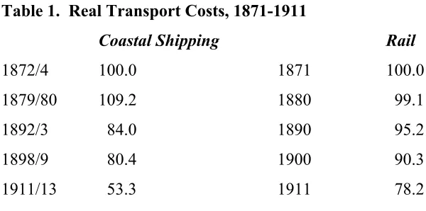
(5) This was a period of falling transport costs.. Initially this was driven by. technological progress in railways and coastal shipping followed by a large-scale move to road freight for distances up to about 125 miles as the internal combustion engine came into its own in the 1920s. Table 1 presents the considerable reduction of costs of both water and railway transport due to improvements in steam technology between 1871 and 1911. <Table 1 about here> While in 1910 coastal shipping accounted for 59 per cent of ton-miles of British freight (Armstrong, 1987) by the 1930s it was unimportant except for a few bulk cargoes. In 1921 road transport accounted for only about 6 percent of ton-miles but this had risen to about 35 per cent in 1939 (Scott, 2002). The transport cost of groceries by rail over a distance of about 90 miles from Birmingham fell in real terms by 18 per cent between 1881 and 1910 and about another 5 per cent by 1925, at which point, however, sending the goods by road would have been only about 33 per cent of the rail cost.1 The main quantitative studies of industrial location in this period are those by Kim (1995) (1998) (1999) for the United States.. He found that the traditional. comparative advantage arguments were the most important determinants of the location of industry and tended to downplay the new economic geography claims. There has not previously been an econometric study of industrial location in Britain in this period. The best informal discussions are probably those of Dennison (1939) and Lee (1971). These. 1. Calculated from BPP (1881), BPP (1910) and Railway Clearing House (1925). A similar rate of decline. for railway transport costs overall is implied by the data in Cain (1980) and Walker (1942).. 2.

(6) authors see a quite dramatic change from the classic industrial revolution experience to that of the interwar years. In the earlier period, much of industry is seen as being tied to raw material inputs, notably coal. In the interwar period, proximity to markets is seen as much more important as, in many industries, firms wanted to be close to their suppliers and their customers with the upshot being a ‘drift to the South’. Dennison concluded that ‘the market is a new factor of primary importance in location’ (1939, 72, emphasis added). However, a pioneering shift-share analysis led the Barlow Commission (Great Britain, 1940) to conclude that the ‘regional problem’ of the interwar period was simply one of an inherited structure in which slow growing/contracting industries which were subject to adverse trends in international trade were concentrated in outer Britain. Accordingly, the question that we address in this paper is whether the new economic geography hypotheses that scale and/or linkage effects influenced the location of British industry prior to World War II can be supported by the empirical evidence. 2. Model All location theories rely on the interaction of location characteristics with the characteristics of economic activities. We employ a variant of Midelfart-Knarvik et al.’s (2000) econometric model of industry location where regions and industry characteristics interact to determine the location of industry. Regions are heterogeneous in various characteristics such as endowments of natural resources and skilled labour and proximity to markets. Similarly, industries differ in their various attributes such as the intensity of use of production factors like natural resources and skilled labour, and their reliance on intermediate inputs. Intuitively, one would then expect that, in an integrated market economy, firms’ profit motive would lead to a regional distribution of industries that is in. 3.

(7) someway determined by the interactions of the various regional and industry characteristics. The rationale for the emphasis on the interaction of industry and country characteristics lies in the general equilibrium nature of the system. Other things equal, every industry may want to locate in a region that is relatively well endowed with skilled labour but a scenario of all industries in a skilled-labour rich region cannot prevail in equilibrium. Hence only industries that are relatively skilled-labour intensive end up in regions that are relatively rich in skilled labour. Therefore, the model’s predictions of industry location entail only the interactions of region and industry characteristics. The first and second columns of Table 2 enumerate the four regional characteristics and the six industrial characteristics, respectively, that will be considered in our econometric analysis. The first three belong to the traditional HO trade model and capture relative endowments of the various production factors.. The last regional. characteristic, market potential is a new economic geography variable that represents a measure of a region’s access to markets (i.e. the proximity advantage of a region). Capital which is the main variable of the HO model in the context of international trade is ignored here because of the assumption of capital mobility nationally. The rationale for taking the variable share of agricultural employment instead of the underlying conventional factor inputs such as land is that, since our concern is the pattern of manufacturing, agriculture can be considered as an exogenous measure of the ‘endowment of agriculture’. Educated population represents the endowment of skilled labour. Since British industry was traditionally very dependent on steam power and coal. 4.

(8) was expensive to transport, coal abundance is included in the list of relevant regional characteristics.2 < Table 2 about here> The first three industrial attributes in the second column of Table 2 are the counterparts of the first three regional characteristics that we have just discussed. They capture the standard factor intensity variables of the HO factor endowment trade models. Three pairs of region and industry characteristics make up the three interaction variables of the factor endowment aspect of the model. The last three industry characteristics belong to the new economic geography literature (Midelfart-Knarvik et al. 2000, 32). Each of them is coupled with the country characteristic of market potential variable to form three interaction variables that represent the new economic geography concerns of the model, namely the pull of centrality. The main hypothesis regarding this pull of centrality is that a firm’s location decision involves consideration of market access besides production costs (see, e.g., Venables, 1996). The first interaction between market potential*intermediate input use represents the notion of forward (or demand) linkage, i.e. as buyers of inputs from other producers, firms with higher shares of such intermediate inputs in costs are likely to locate in central locations in order to minimize transport costs. This pull of centrality driven by firms’ optimization behaviour can only materialise if transport costs are not very high since high. 2. Midelfart-Knarvik et al. (2000) include a research and development variable in their list of regional and. industry characteristics. We omit this because for most of our period expenditure on research and development was tiny; even in the mid 1930s it was less than 0.5 per cent of GDP (Edgerton and Horrocks, 1994).. 5.

(9) transport costs would raise the cost of reaching final consumers (see, e.g., Krugman, 1991b, 51-52 and Venables, 1996). If falling transport costs reached the ‘intermediate zone’ in pre-1931 Britain, we expect the sign of this interaction to be positive. The second interaction variable, market potential*industry sale, depicts a similar notion of backward (or supply) linkage, i.e. industries with higher shares of their output sold to other producers tend to locate near central locations (i.e. regions of high market potential) to be close to these other producers. The direction or sign of this interaction cannot be determined a priori since it depends on whether proximity to industrial customers pays more than proximity to final consumers. In other words, while the supply linkage exerts a force for clustering of industries, the location of final consumer demand would work in the opposite direction (Venables, 1996, 342). The third and last interaction variable, market potential*size of establishment depicts the hypothesis that industries with relatively high scale economies tend to locate in regions of high market potential. The reason is that firms with increasing-returns-toscale technology would face a trade-off between minimization of transport costs (that can be achieved by locating in scattered areas and operating at a smaller scale) and the advantage of large scale production by locating in central locations and supplying from these central areas, and this trade-off is likely to result in the “…emergence of a lattice of ‘central places’…” (Fujita, et al. 1999, 26; see also Krugman, 1991a, 485-486). Falling transport costs may lessen this trade-off and induce such firms to be close to central locations. However, the pull of centrality with regard to firms with scale economies weakens when transport costs fall below intermediate levels unless the vertical linkage between industries is substantial as firms would then be relatively more sensitive to. 6.

(10) production cost differences than to ease of market access (Venables, 1996). If there is a pull of centrality based on scale economies, then the interaction term between market potential and economies of scale should be positive. Formally, the model is specified as:. ln(s ik ) = α ln( popi ) + β ln(mani ) + ∑ j β [ j ]( y[ j ]i − γ [ j ]( z[ j ] k − κ [ j ]). where. (1). s ik is the share of region i in the total British manufacturing employment in. industry k; popi is the share of Britain’s population living in region i; mani is the share of Britain’s manufacturing employment located in region i; y[ j ]i is the level of the jth regional characteristic in region i;. z[ j ] k is the industry k value of the industry. characteristic paired with regional characteristic j (see Table 2); and α , β , β [ j ] , γ [ j ] and κ [ j ] are coefficients to be estimated. The distinguishing feature of this econometric model is twofold: the nesting of two major forces of industry location corresponding to two major strands of literature (namely, the HO factor endowment and the new economic geography models) and the modelling of the theoretically-emphasized joint role of regional and industry characteristics in the determination of the pattern of industry location. Specifically, what the model says is that after controlling for regional size effects (via the first two variables) i.e. the hypothesis that a regional share of industrial employment increases with the size of the region, the pattern of industry is shaped by the interactions between the region and industry characteristics. The interaction forces are represented by the terms in the summation.. 7.

(11) For a more specific discussion of these interaction forces, we reproduce here Midelfart-Knarvik et al.’s illustration of the meaning of their model by means of a specific example, say, skilled labour. So z[skilled labour]k is skilled-labour intensity of industry k and y[skilled labour]i is skilled-labour abundance of region i. The following interpretation can then be given to the model: A) There exists an industry with a cut-off level of skilled-labour intensity k[skilled labour] such that its location is independent of regional skilled-labour abundance; B) There exists a cut-off level of skilled-labour abundance γ[skilled labour] such that the region’s share of any industry is independent of the skilled-labour intensity of the industry; and C) If β[skilled labour] > 0, then industries with skilled-labour intensity greater than the cut-off point, i.e. k[skilled labour] will be induced to locate near regions with skilled-labour abundance greater than the cut-. off point, i.e. γ[skilled labour] and away from regions with skilled-labour abundance less than this cut-off point. More generally what the model says is that with falling transport costs (implying closer integration), industries move to exploit comparative advantages, and scale/agglomeration economies. How does this model accomplish the purpose of testing these hypotheses? The model is confronted with data from a period when transport costs were decreasing considerably. Hence, the overall fit of the model to the data and the significance of individual coefficients will help us assess these hypotheses. Moreover, when the model is estimated for different time periods over which transport costs were declining, we will have the opportunity for a further experiment with respect to our main question set out in the previous section: at what point did new economic geography factors begin to matter?. 8.

(12) Obviously, the model as it stands in (1) does not lend itself to econometric estimation. We, therefore, employ its expanded form as follows:. ln(sik ) = α ln( popi ) + β ln(mani ) +. ∑ ( β [ j ]( y[ j ] z[ j ] j. i. k. − β [ j ]γ [ j ]z[ j ] k − β [ j ]κ [ j ] y[ j ]i ). (2). Estimation of Equation (2) produces the parameters of interest that may be related to our description of the model in (1) as follows. The coefficients of the two size variables, α , β are straightforward. The estimated coefficients of the regional characteristics, y[ j ]. and the industry characteristics, z[ j ] are estimates of − β [ j ]κ [ j ] and − β [ j ]γ [ j ] , respectively. The estimated coefficients of the interaction variables, y[ j ]z[ j ] would be estimates of β [ j ] . If we divide the regional characteristics coefficients, − β [ j ]κ [ j ] by β [ j ] we obtain estimates of the cut-off points for each industry characteristic. Similarly,. dividing the coefficients of the industry characteristics, − β [ j ]γ [ j ] , by β [ j ] gives estimates of the cut-off points for each regional characteristic. As pointed out above the model’s prediction of industry location patterns is entirely on the basis of the interaction terms. Hence, the crucial set of parameters in the model is β [ j ] . The relative magnitude and statistical significance of this coefficient on, say, for example, educated. population*white collar workers provides us with a measure of how important this factor endowment was in influencing the location of industries in pre-1931 Britain.. We. estimate Equation (2) for each of the seven census years from 1871 to 1931 using Ordinary Least Squares (OLS).. 9.

(13) 3. Data. Data sources are listed in the appendix. In this section, we discuss aspects that raise some difficulty and then go on to provide some basic descriptive statistics that will provide the context for the econometric estimation of the following section. With respect to industry characteristics, as is common in research of this type, estimates of the inputoutput relationships which are central to the new economic geography hypotheses are only available at intervals rather than for each census year. In fact, the first Census of Production was not held until 1907. Thomas (1984) derived a full 36 sector input-output table from that source and we have used his results to obtain data on the ratios of intermediate inputs to gross output and of sales to industry as a proportion of gross output for 1871-1911.3 For the interwar period, an input-output table of similar size was derived by Barna (1952) from the 1935 Census of Production this is our source for 1921 and 1931. Other industry characteristics including establishment size, use of steam power and of white-collar workers are also observed only once prior to World War I, in 1907, and these are taken to apply to all the years 1871 through 1911. For the interwar period the Censuses of Production of 1924 and 1930 allow separate estimates for each of 1921 and 1931. With respect to regional characteristics time varying information is available for all variables except coal abundance. Evidence on the retail price of coal at the regional. 3. Charles Feinstein will shortly publish an input-output table for 1851. He has generously made available. to us his estimates and we re-ran all our regressions using them instead of the Thomas estimates. This made no material difference to our results.. 10.

(14) level is quite thin but at the same time the pattern of high and low price areas appears to have been quite stable and was based on proximity to coalfields. We have used evidence from two parliamentary enquiries which provide data for 1840, 1905 and 1912. Employment data are straightforward thanks to the work of Lee (1979) who organized the original Census data into a 2-digit industrial classification for the standard British regions. The dependent variable and the two size variables also come from this source. Data on years of schooling at the regional level are not available for the pre World War I period so we have used the proportion of workers in the labour force as a whole classified by the Census as Professional or Financial and Commercial (categories III and V). For 1921 and 1931, there is information available on years of schooling by age group in the 1951 which permits a retrospective view of the education of the median worker (by age). Market potential is based on the measure used by Keeble et al. (1982). It is defined as Pi = ΣGDPjdγij where Pi is the potential of region i and d is the distance between region i and region j. γ is traditionally set at − 1. Own distance is approximated by the formula dii = 0.333√(area of region/π). Thus market potential depends on a distance-deflated sum of neighbouring regions’ GDP and own GDP.. Constructing. estimates of market potential entailed first making estimates of British regional GDP using the method proposed by Geary and Stark (2002); these estimates are further. 11.

(15) discussed in the data appendix.4 GDP of neighbouring countries is taken into account in a similar fashion. < Table 3 about here> Distances are based both on land and sea with sea miles converted into a land equivalent based on relative costs. From 1871 to 1921 it is assumed that all land transport was by rail; in these years, if coastal shipping was cheaper (as for journeys from London to Scotland, for example), this was assumed to have been the preferred mode. In 1931, road haulage was assumed to have been used for land journeys up to 130 miles and conversion factors were obtained based on costs for rail transport for longer distances and for sea transport to foreign countries. Further details can be found in Crafts (2004b).5 The switch to road haulage for short and medium distance transport had the implication that the landlocked midlands suddenly became much “closer” to London and the South East while outer Britain was now “further away”. This is reflected in the estimates of market potential relative to London & South East reported in Table 3.. 4. It is possible to refine these estimates further for the pre World War I period by taking account of the. geographical spread of income tax receipts. This leads to modest changes in market potential across regions with the relative level of London & South East rising. Incorporating this modification makes no difference to our econometric results so we have preferred to base market potential on estimates of regional GDP constructed on a consistent basis through out. 5. In principle, an alternative procedure would be to work with estimated gravity models of trade. This was. rejected because there is no data on regional trade flows and it would be impossible to capture the sense of Birmingham becoming closer to London with the advent of road haulage.. 12.

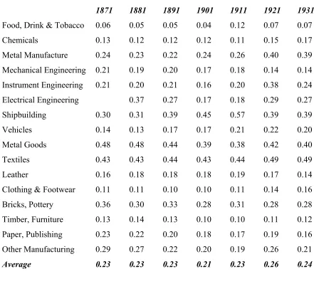
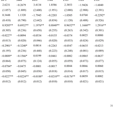
(16) < Table 4 about here> Table 4 reports coefficients of localization for the 16 2-digit industries used in the econometric estimation. Among the notable results are the high concentration of textiles, a traditional sector which was a big user of steam power, and increasing concentration in vehicles, a sector that included a major new industry that increasingly located in the south east and the midlands. Nevertheless, in many sectors localization in 1931 was still similar to 1871 and the average across industries did not vary greatly over time. Table 5 reports the average value across the regions of an index of regional specialization. This was decreasing slowly in the late nineteenth century but then shows a substantial increase across World War I. This bears some similarity to calculations for the United States in Kim (1995) but the phase of increased specialization arrives a decade or so later and is much weaker. < Table 5 about here> 4. Estimation Results. Table 6 reports the results from estimation of the model in (2) for the ten British regions for the period 1871-1931. The estimated coefficients of the intercept term and the two size variables appear in the first three rows followed by the coefficients of the four regional characteristics, y[ j ] , the six industry characteristics, z[ j ] and finally the six interaction variables, β [ j ] . As has already been noted, since this is a model of a general equilibrium type the estimated coefficients of the regional and industry characteristics are hardly of any interest. The focus is on the coefficients of the interaction variables that capture the joint role of regional and industry characteristics in the movement of industry. < Table 6 about here> 13.

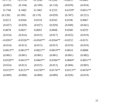
(17) Of the two size variables, manufacturing employment always has the right sign and is generally quite close to unity. In almost all cases, the coefficients of the regional characteristics have the expected negative signs but are usually statistically insignificant. With respect to the industry characteristics, the coefficients of the variables share of. agricultural employment, educated population and size of establishment have the expected negative signs and are significantly different from zero for 1871 to 1911 in each case. Turning to the crucial variables of the model, we see that the coefficients of the interaction variables involving the traditional factor endowment variables have the right signs. Educated population*white collar workers and coal abundance*steam power use are statistically different from zero throughout and from 1871 to 1911 share of. agricultural employment*agricultural input use is significant. The importance of the traditional factor endowment variables in the pattern of industry location in pre-1931 Britain is confirmed by these results. With respect to the coefficients of the interaction variables involving the new economic geography forces, market potential*intermediate input use and market. potential*industry sale generally have the wrong signs but are always insignificant. Market potential*size of establishment has the expected positive sign and is statistically significant from 1871 to 1911. There is a clear pattern that the coefficient on this variable is declining. This suggests that the pull of centrality for increasing returns. 14.

(18) industries was weakening over time and in this regard transport costs may have fallen below the ‘intermediate’ range by the interwar period.6 By way of comparing the relative importance of the factor endowment factors and the scale economy aspect of the new economic geography models, we could make use of beta coefficients, i.e. adjusted regression coefficients which are all in the same unit, thus are comparable. Such an exercise reveals that on average during the sample period, the market interaction/size of establishment variable scores first followed by the factor endowment interaction variables of educated population/white collar workers, coal abundance/steam power use and agricultural employment/agricultural input use. Nonetheless, looking at the factor endowment factors as a whole the average beta coefficient turns out to be 1.05 against 0.72 for the market potential/size of establishment interaction variable.. 6. We have explored alternative econometric specifications to estimate our data set by pooling the seven sets. of cross-section data. Two sets of estimators that we considered are: the pooled least square estimator that represents the average of the within-groups and between-groups estimators; and least square estimators with region or sector specific effects or/and period specific effects that represent within-group estimators. Each of these leaves the regression results more or less intact. The exception is the market potential/size of establishment interaction variable, which changes its sign and losses its significance. This is probably not surprising in view of the observation we have made that the importance of this force has been changing over time. A further experiment by restricting the sample period to 1871-1911 (where the pull of centrality on establishment size was statistically significant) shows that the alternative estimators do not result in any material changes to our results. All these results of alternative specifications are available from the authors upon request.. 15.

(19) In sum, these results give much greater support to explanations for industry location based on the traditional Heckscher-Ohlin model rather than those derived from the new economic geography. In particular, neither of the linkage effects interaction variables are significant at any point between 1871 and 1931 while the factor endowment interaction variables show up strongly throughout. There is support for the pull of centrality for industries with greater establishment size but, interestingly, this appears to have been decreasing through time.7 5. Discussion. The main thrust of our results is that factor endowments played the central role in industry location decisions before World War II. In particular, the continuing roles of natural resources in terms of coal abundance and of human capital are apparent. The former matches quite closely the central findings of investigations into the location of American manufacturing and regional specialization in the United States at this time. Kim (1998) concluded that the main influence was that industry was moving to largescale production methods that were intensive in the use of relatively immobile energy resources.. Kim (1995) also discounted new economic geography explanations that. focused on external economies but he did not explicitly examine the linkages arguments. We do not find any evidence of a new pull of centrality in industrial location decisions in the interwar period. Therefore, unlike Dennison (1939) we do not believe that the ‘regional problem’ of those years should be linked to the emergence of industries. 7. We also experimented with a specification that allows interactions between market potential and the scale. economy variable and the linkages variables. These variables were insignificant.. 16.

(20) whose location decisions were dominated by linkage effects which made them wish to be close to their suppliers and/or customers. The diagnosis of the Barlow Commission (Great Britain, 1940) seems to be nearer the mark, namely, that the difficulties of the Victorian staple industries were the heart of the matter rather than any new disadvantage to outer Britain arising from changing transport costs. It is also interesting to consider our results in the context of those for European Union regions in the period 1970-1997 by Midelfart-Knarvik et al. (2000). They found rather more support for new economic geography linkage effects but not before the 1990s while in their study the coefficient on the interaction between market potential and scale economies was significant from 1970 to 1990 but declining in magnitude and eventually insignificant in 1997. This implies that falls in transport costs permitting increasing returns industries to serve markets from less central locations have occurred across Europe in the recent past but must have started to prevail earlier within Britain which was, of course, a much more integrated economy. Taken together, the results of these two papers suggest that linkage effects were a relatively weak influence on location decisions until the very recent past. 6. Conclusions. This paper sets out to explain the location of industry in Britain in the years 1871 to 1931. We explore seven sets of cross-section data from 1871-1931 using an econometric model of industry location that nests both the HO factor endowment and new economic geography models. This model pioneered by Midelfart-Knarvik et al. (2000) stresses the general equilibrium nature of the system and allows regional and industry characteristics to interact in the determination of industrial location.. 17.

(21) The results indicate that traditional factor endowment arguments were the main explanation of location decisions throughout the period 1871 to 1931. We also found a role for the pull of centrality through market potential interacting with scale economies but to a decreasing extent as transport costs fell over time such that by 1931 it is no longer statistically significant. Transport costs were, however, apparently not yet low enough to allow the linkage effects highlighted by the new economic geography to emerge as a factor in location decisions.. 18.

(22) Appendix. Data sources are as follows:. -. Input-output data (intermediate inputs/gross output, agricultural inputs/ gross output, sales to industry/gross output in %) for 1871-1911 from Thomas (1984) derived from 1907 Census of Production and for 1921-1931 from Barna (1952) derived from 1935 Census of Production.. -. Establishment size for 1871-1911 based on employment per plant from returns under the Factory and Workshop Act for 1907 (BPP 1909) and for 1921 based on 1924 Census of Production and for 1931 based on 1930 Census of Production.. -. White Collar Workers/Employment based on Administrative, Technical and Clerical Workers as percentage of total employees for 1871-1911 from 1907 Census of Production, for 1921 from 1924 Census of Production and for 1931 from 1930 Census of Production.. -. Steam Power based on steam horsepower/gross output from 1907 Census of Production for 1871-1911, from 1924 Census of Production for 1921 and from 1930 Census of Production for 1931.. -. Educated population for 1871-1911 from Census of Population based on employment in categories III and V (%) and for 1921 and 1931 derived from the 1951 Census of Population based on education to 15 or more based on age 65-74, and age 55-64 respectively.. -. Employment in agriculture, manufacturing and population in British regions from Lee (1979).. -. Coal Abundance based on coal prices from BPP (1843) and BPP (1912/13).. 19.

(23) Regional GDP estimates which underlie the Market Potential estimates have been constructed using the method proposed by Geary and Stark (2002). Briefly this uses data on employment structure (agriculture, industry, services) and sectoral wages together with estimates of UK output for each sector.. It assumes that regional sectoral. productivity relative to the UK average is reflected in regional sectoral wages relative to the UK average. UK GDP is defined as YUK = ΣYi where Yi is GDP of region i which is in turn defined as Yi = ΣyijLij where yij is average value-added per worker in region i in sector j and Lij is the corresponding number of workers. Then assume that Yi = Σ[yjβj(wij/wj)]Lij where yj is UK output per worker in sector j, wij is the wage paid in region i in sector j and wj is the national average wage in sector j. β is a scalar which preserves the relative regional differences but scales the absolute levels so that regional totals for each sector sum to the known UK total. Full details of the wage data used to implement the GearyStark method can be found in Crafts (2004a). These estimates for regional GDP have been supplemented by estimates at current exchange rates of the GDP in main trading partners including all western European countries derived using the data in Prados de la Escocura (2000). To move to market. potential the standard formulae in Keeble et al. (1982) were employed and distances were 20.

(24) obtained from Dataloy Systems at www:dataloy.com/newwebsite/index.php and. Bradshaw’s Railway Guide. Full details can be found in Crafts (2004b).. Acknowledgment. Financial support from the Economic and Social Research Council under grant R000239536 is gratefully acknowledged. We wish to thank Steve Redding for helpful comments and suggestions on an earlier version of this paper. The usual disclaimer applies.. 21.

(25) References. Armstrong, J. (1987) The Role of Coastal Shipping in UK Transport: an Estimate of Comparative Traffic Movements in 1910, Journal of Transport History, 8: 164178. Barna, T. (1952) The Interdependence of the British Economy, Journal of the Royal. Statistical Society, 115: 29-81. British Parliamentary Papers (1843) An Account of the Prices at Poor Law Unions, vol. XLV. British Parliamentary Papers (1881) Report of the Select Committee on Railways, vol. XIV. British Parliamentary Papers (1909) Summary of Returns under the Factory and Workshop Act, vol. LXXIX. British Parliamentary Papers (1910) Report of the Royal Commission on Canals and Railways, vol. XII. British Parliamentary Papers (1912/13) Cost of Living of the Working Classes, vol. LXVI. Cain, P. J. (1980) Private Enterprise or Public Utility?: Output, Pricing and Investment on English and Welsh Railways, 1870-1914, Journal of Transport History, 1: 9-28. Crafts, N. (2004a) Regional GDP in Britain, 1871-1911: Some Estimates. Department of Economic History Working Papers in Large Scale Technological Change No. 01/04, London School of Economics.. 22.

(26) Crafts, N. (2004b) Market Potential in British Regions, 1871-1931. Department of Economic History Working Papers in Large Scale Technological Change No. 02/04, London School of Economics. Dennison, S. (1939) The Location of Industry and the Depressed Areas. London: Oxford University Press. Edgerton, D. E. H. and Horrocks, S. (1994) British Industrial Research and Development before 1945, Economic History Review, 47: 213-238. Fujita, M., Krugman, P. and Venables, A. J. (1999) The Spatial Economy, Cities, Regions. and International Trade. Cambridge, Mass.: MIT press. Geary, F. and Stark, T. (2002) Explaining Ireland’s Post-Famine Economic Growth Performance, Economic Journal, 112: 919-935. Great Britain (1940) Report of the Royal Commission on the Distribution of the Industrial Population (Cmd. 6153). Keeble, D., Owens, P. L. and Thompson, C. (1982) Regional Accessibility and Economic Potential in the European Community, Regional Studies, 16: 419-432. Kaukiainen, Y. (2003) How the Price of Distance Declined: Ocean Freights for Coal and Grain from the 1870s to 2000. Mimeo, University of Helsinki. Kim, S. (1995) Expansion of Markets and the Geographic Distribution of Economic Activities: the Trends in US Regional Manufacturing Structure, 1860-1987,. Quarterly Journal of Economics, 110: 881-908. Kim, S. (1998) Economic Integration and Convergence: US Regions, 1840-1987, Journal. of Economic History, 58: 659-683.. 23.

(27) Kim, S. (1999) Regions, Resources, and Economic Geography: Sources of US Regional Comparative Advantage, 1880-1987, Regional Science and Urban Economics, 29: 1-132. Krugman, P. (1991a) Increasing Returns and Economic Geography, Journal of Political. Economy, 99: 183-199. Krugman, P. (1991b) Geography and Trade. Cambridge, Mass: MIT Press. Krugman, P. and Venables, A. J. (1995) Globalization and the Inequality of Nations,. Quarterly Journal of Economics, 110: 857-880. Lee, C. H. (1971) Regional Economic Growth in the United Kingdom since the 1880s. London: McGraw-Hill. Lee, C. H. (1979) British Regional Employment Statistics, 1841-1971. Cambridge: Cambridge University Press. Midelfart-Knarvik, H., Overman, G., Reading, J. and Venables, J. (2000) The Location of European Industry, Economic Papers No. 142 European Commission, D-G for Economic and Financial Affairs, Brussels. Prados de la Escocura, L. (2000) International Comparisons of Real Product, 1820-1990: an Alternative Data Set, Explorations in Economic History, 37: 1-41. Railway Clearing House (1925) Report on Road Motor Transport in Relation to the Railways. Public Record Office RAIL 1080/672. Scott, P. (2002) British Railways and the Challenge from Road Haulage, Twentieth. Century British History, 13: 101-120. Thomas, M. (1984) An Input-Output Approach to the British Economy, 1890-1914. Oxford D. Phil. Thesis.. 24.

(28) Venables, A. J. (1996) Equilibrium Locations of Vertically Linked Industries,. International Economic Review, 37: 341-359. Walker, G. (1942) Road and Rail. London: Allen and Unwin.. 25.

(29) Table 1. Real Transport Costs, 1871-1911 Coastal Shipping. Rail. 1872/4. 100.0. 1871. 100.0. 1879/80. 109.2. 1880. 99.1. 1892/3. 84.0. 1890. 95.2. 1898/9. 80.4. 1900. 90.3. 1911/13. 53.3. 1911. 78.2. Sources: coastal shipping based on a distance of 400 miles from Kaukiainen, (2003); rail based on. average rates per ton per mile from Cain, (1980).. 26.

(30) Table 2. Regional and Industry Characteristics Regional characteristics. Industry characteristics. Share of agricultural employment Educated proportion of the labour force. Agricultural inputs as a percentage of gross output White-collar workers as a percentage of employment. Coal abundance. Steam power use. Market potential. Intermediates as a percentage of gross output in industry Sales to industry as percentage of output Size of establishment. The regions are ten standard British regions: London and Rest of South East, East Anglia, South West, West Midlands, East Midlands, North West, Yorkshire and Humber, North, Wales and Scotland. There are 16 two-digit industries (15 in 1871): Food, Drink and Tobacco; Chemicals; Metal Manufacture; Mechanical Engineering; Instrument Engineering; Electrical Engineering; Shipbuilding and Marine Engineering; Vehicles; Metal Goods; Textiles; Leather; Clothing and Footwear; Bricks, Pottery, Glass and Cement; Timber and Furniture; Paper, Printing and Publishing; and Other Manufacturing.. 27.

(31) Table 3. Market Potential Relative to London & South East (%) 1871. 1881. 1891. 1901. 1911. 1921. 1931. East Anglia. 63.8. 63.9. 64.0. 63.9. 65.6. 62.7. 59.1. South West. 73.2. 74.2. 77.0. 74.5. 75.3. 71.1. 66.4. West Midlands. 67.4. 67.2. 65.0. 60.4. 60.8. 71.5. 68.2. East Midlands. 62.2. 61.2. 60.0. 55.3. 55.9. 66.0. 62.9. North West. 97.8. 99.0. 97.5. 90.0. 89.2. 100.8. 94.5. Yorks & Humb. 74.8. 74.9. 73.9. 70.2. 70.1. 78.5. 74.8. North. 66.0. 67.7. 71.4. 72.5. 72.4. 66.1. 57.6. Wales. 70.1. 72.8. 74.9. 75.4. 76.2. 69.5. 63.5. Scotland. 66.0. 63.4. 66.3. 68.1. 67.5. 60.3. 51.5. Source: own calculations, see text and Crafts (2004b). The estimates in this table use estimates of. regional GDP based on the Geary-Stark (2002) method.. 28.

(32) Table 4. Localization Indices, 1871-1931 1871. 1881. 1891. 1901. 1911. 1921. 1931. Food, Drink & Tobacco. 0.06. 0.05. 0.05. 0.04. 0.12. 0.07. 0.07. Chemicals. 0.13. 0.12. 0.12. 0.12. 0.11. 0.15. 0.17. Metal Manufacture. 0.24. 0.23. 0.22. 0.24. 0.26. 0.40. 0.39. Mechanical Engineering. 0.21. 0.19. 0.20. 0.17. 0.18. 0.14. 0.14. Instrument Engineering. 0.21. 0.20. 0.21. 0.16. 0.20. 0.38. 0.24. 0.37. 0.27. 0.17. 0.18. 0.29. 0.27. Electrical Engineering Shipbuilding. 0.30. 0.31. 0.39. 0.45. 0.57. 0.39. 0.39. Vehicles. 0.14. 0.13. 0.17. 0.17. 0.21. 0.22. 0.20. Metal Goods. 0.48. 0.48. 0.44. 0.39. 0.38. 0.42. 0.40. Textiles. 0.43. 0.43. 0.44. 0.43. 0.44. 0.49. 0.49. Leather. 0.16. 0.18. 0.18. 0.18. 0.19. 0.17. 0.14. Clothing & Footwear. 0.11. 0.11. 0.10. 0.10. 0.11. 0.14. 0.16. Bricks, Pottery. 0.36. 0.30. 0.33. 0.28. 0.31. 0.28. 0.28. Timber, Furniture. 0.13. 0.14. 0.13. 0.10. 0.10. 0.11. 0.12. Paper, Publishing. 0.23. 0.22. 0.20. 0.18. 0.17. 0.19. 0.16. Other Manufacturing. 0.29. 0.27. 0.22. 0.20. 0.19. 0.26. 0.21. Average. 0.23. 0.23. 0.23. 0.21. 0.23. 0.26. 0.24. Source: derived from Lee (1979); Coefficient of Localization = Σ(si − smanf) for all positive. values where si is a region’s share of employment in industry i and smanf is the region’s share of all manufacturing.. 29.

(33) Table 5. Average Krugman Index of Regional Specialization. 1871. 0.66. 1881. 0.64. 1891. 0.64. 1901. 0.59. 1911. 0.61. 1921. 0.79. 1931. 0.72. Source: derived from Lee (1979), average of 10 standard regions.. 30.

(34) Table 6. British Industry Location Regressions, 1871-1931 1871. Constant Population Manufacturing Employment Share of Agricultural Employment Educated Population Coal Abundance Market Potential Agricultural Input Use. 1881. 1891. 1901. 1911. 1921. 1931. 2.6231. −0.2679. 3.4134. 1.8586. 2.3853. −1.9426. −1.6040. (1.057). (1.889). (2.600). (1.951). (2.088). (2.988). (2.391). 0.3448. 1.1320. −1.7945. −0.2203. −1.0505. 0.0768. −0.2292*. (0.418). (0.790). (2.642). (0.854). (1.120). (0.488). (0.526). 0.9205**. 0.6932**. 1.1976**. 0.8840**. 0.9652**. 1.1660**. 1.2916**. (0.305). (0.236). (0.658). (0.255). (0.263). (0.342). (0.301). −0.0094. −0.0534. −0.0155. −0.0374. 0.0025. 0.0080. (0.013). (0.020). (0.046). (0.020). (0.033). (0.024). (0.029). −0.2901*. −0.3240*. 0.0814. −0.2263. −0.0547. −0.0635. −0.0213. (0.195). (0.236). (0.448). (0.223). (0.248). (0.081). (0.089). −0.0889*. −0.1566*. 0.0199. −0.0461. −0.0082. −0.0865. −0.0637. (0.064). (0.075). (0.124). (0.055). (0.059). (0.073). (0.077). −0.0475. −0.0001. −0.0017. 0.0044. 0.0066. 0.0060. (0.050). (0.045). (0.038). (0.018). (0.014). (0.017). (0.015). −0.0227**. −0.0224**. −0.0188*. −0.0210**. −0.0176**. 0.0059. 0.0082. (0.012). (0.012). (0.012). (0.010). (0.010). (0.021). (0.021). −0.0227*. −0.0784*. Continued on next page. 31.

(35) Table 6 continued White Collar Workers Steam Power Use. 1871. 1881. 1891. 1901. 1911. 1921. 1931. −0.2920**. −0.1752**. −0.3110**. −0.3286**. −0.3202**. −0.0651**. −0.0401*. (0.100). (0.093). (0.104). (0.109). (0.110). (0.039). (0.034). 0.0869. 0.1768. 0.1802. 0.1965. 0.2333. 0.6339*. 0.6011**. (0.029). (0.307). (0.221). (0.109) Intermediate Input Use. (0.120). (0.109). (0.119). 0.0218. 0.0213. 0.0304. 0.0318. 0.0343. 0.0196. 0.0067. (0.025). (0.027). (0.029). (0.027). (0.029). (0.049). (0.041). 0.0006. 0.0078. 0.0037. 0.0055. 0.0048. 0.0308. 0.0255. (0.013). (0.014). (0.016). (0.015). (0.017). (0.022). (0.019). −0.0215*. −0.0201*. −0.0326**. −0.0345**. −0.0364**. −0.0232. −0.0151. (0.013). (0.014). (0.013). (0.013). (0.015). (0.019). (0.018). Share of Agricultural Employment. 0.0014**. 0.0015**. 0.0015**. 0.0021**. 0.0019**. 0.0018. 0.0008. *Agricultural Input Use. (0.001). (0.001). (0.001). (0.001). (0.001). (0.001). (0.002). Educated Population*White Collar. 0.0490**. 0.0320**. 0.0415**. 0.0465**. 0.0386**. 0.0069*. 0.0051**. Workers. (0.015). (0.014). (0.013). (0.015). (0.013). (0.004). (0.003). Coal Abundance*Steam Power. 0.0079. 0.0155**. 0.0153**. 0.0150**. 0.0176**. 0.0513**. 0.0476**. Use. (0.009). (0.009). (0.008). (0.009). (0.009). (0.028). (0.019). Industry Sale Size of Establishment. Continued on next page. 32.

(36) Table 6 continued 1871. 1881. 1891. 1901. 1911. 1921. 1931. −0.0005. −0.0004. −0.0004. −0.0003. −0.0003. −0.0001. −0.0001. (0.001). (0.001). (0.0005). (0.0003). (0.0002). (0.0002). (0.0002). 0.00004. −0.0001. −0.0001. −0.0001. −0.0001. −0.0002. −0.0001. (0.003). (0.0003). (0.0003). (0.0002). (0.0001). (0.0001). (0.0001). Market Potential*Size of. 0.0006**. 0.0004*. 0.0005*. 0.0004**. 0.0001. 0.0001. Establishment. (0.0003). (0.0003). (0.0002). (0.0001). (0.0001). (0.0001). (0.0001). Market Potential*Intermediate Input Use Market Potential*Industry Sale. 0.0003**. Observations. 150. 160. 160. 160. 160. 160. 160. Adjusted R2. 0.57. 0.59. 0.64. 0.66. 0.65. 0.56. 0.62. Notes: Heteroskedasticity-robust standard errors in parenthesis. * is significant at 10% level. ** is significant at 5% level.. 33.

(37)

No results found