Quantification of the plant endoplasmic reticulum

University of Warwick institutional repository: http://go.warwick.ac.uk/wrap

A Thesis Submitted for the Degree of PhD at the University of Warwick

http://go.warwick.ac.uk/wrap/2742

This thesis is made available online and is protected by original copyright. Please scroll down to view the document itself.

THE UNIVERSITY OF WARWICK

Molecular Organisation and Assembly in Cells

(MOAC)

Quantification of the Plant Endoplasmic

Reticulum

PhD. Thesis

Abdnacer Bouchekhima

THE UNIVERSITY OF WARWICK

Molecular Organisation and Assembly in Cells

(MOAC)

Centre for Scientific Computing(CSC)

Mathematics Institute

Department of Biological Sciences

Quantification of the Plant Endoplasmic

Reticulum

by

Abdnacer Bouchekhima

Supervisors

Dr. Lorenzo Frigerio

Department of Biology

Dr. Markus Kirkilionis

Mathematics Institute

This thesis is submitted in partial fulfilment of the requirements for

the degree of

Doctor of Philosophy in Scientific Computing

September 7, 2009

c

Abstract

One of the challenges of quantitative approaches to biological sciences is the lack of understanding of the interplay between form and function. Each cell is full of complex-shaped objects, which moreover change their form over time. To address this issue, we exploit recent advances in confocal microscopy, by using data collected from a series of optical sections taken at short regular intervals along the optical axis to reconstruct the Endoplasmic Reticulum (ER) in 3D, obtain its skeleton, then associate to each of its edges key geometric and dynamic characteristics obtained from the original filled in ER specimen. These properties include the total length, surface area, and volume of the ER specimen, as well as the length surface area, and volume of each of its branches. In a view to benefit from the well established graph theory algorithms, we abstract the obtained skeleton by a mathematical entity that is a graph. We achieve this by replacing the inner points in each edge in the skeleton by the line segment connecting its end points. We then attach to this graph the ER geometric properties as weights, allowing therefore a more precise quantitative characterisation, by thinning the filled in ER to its essential features. The graph plays a major role in this study and is the final and most abstract quantification of the ER. One of its advantages is that it serves as a geometric invariant, both in static and dynamic samples. Moreover, graph theoretic features, such as the number of vertices and their degrees, and the number of edges and their lengths are robust against different kinds of small perturbations. We propose a methodology to associate parameters such as surface areas and volumes to its individual edges and monitor their variations with time. One of the main contributions of this thesis is the use of the skeleton of the ER to analyse the trajectories of moving junctions using confocal digital videos. We report that the ER could be modeled by a network of connected cylinders (0.87µm_±0.36 in diameter) with a majority of 3-way junctions. The average length, surface area and volume of an ER branch are found to be 2.78_±2.04µm, 7.53_±5.59µm2_{and 1.81±1.86µm}3 _{respectively. Using the analysis of}

Acknowledgments

Contents

List of Figures xv

List of Tables xvii

List of Algorithms xix

Nomenclature xxi

I

Background

1

1 Thesis road map 3

2 Motivations 7

2.1 Introduction . . . 8

2.2 The ER visualised by confocal microscopy . . . 9

2.3 The ER visualised by electron microscopy . . . 11

2.4 How the ER gets its form . . . 13

2.5 The ER and the Secretory Pathway . . . 15

2.6 The role of the ER in protein folding . . . 16

2.7 The ER and quality control . . . 18

2.8 The ER and Golgi bodies . . . 19

2.9 The plant ER . . . 20

2.10 Common Techniques to study the ER . . . 21

2.10.1 Agrobacterium-mediated transformation . . . 21

2.11 Chapter Summary . . . 23

II

Methodology

25

3 Data Acquisition 27

3.1 Introduction . . . 28

3.2 Sample preparation . . . 29

3.3 Confocal microscopy . . . 30

3.3.1 An overview . . . 31

3.3.2 The objective . . . 35

3.3.3 The pinhole . . . 37

3.3.4 Optical resolution power . . . 38

3.3.5 Optimal voxel size . . . 46

3.4 Noise in confocal images . . . 47

3.5 Chapter Summary . . . 51

4 Skeleton Extraction 53 4.1 Introduction . . . 54

4.2 Terminology . . . 55

4.3 Data pre-processing . . . 58

4.3.1 Z-Drop correction . . . 59

4.3.2 The median filter . . . 60

4.3.3 The Gaussian filter . . . 61

4.4 Binarisation . . . 61

4.4.1 Global thresholding . . . 62

4.4.2 Adaptive thresholding . . . 63

4.5 Skeleton extraction methods . . . 63

4.5.1 Continuous methods . . . 64

4.5.2 Discrete methods . . . 67

4.6 Distance transforms . . . 73

4.6.1 Exact Euclidean distance transformations . . . 74

4.6.2 Approximate distance transformations . . . 75

4.6.3 Chamfer masks . . . 79

4.7 Chapter Summary . . . 82

5 Motion Analysis 83 5.1 Introduction . . . 84

5.2 Point tracking algorithm . . . 85

5.2.1 Image restoration . . . 86

5.2.2 Estimating point locations . . . 88

5.2.3 Refining point locations . . . 89

5.2.4 Non-particle discrimination . . . 90

5.3 Chapter Summary . . . 93

6 Data Abstraction 95 6.1 Introduction . . . 96

6.2 Length of the skeleton . . . 97

6.3 Surface area of the specimen . . . 97

6.4 The volume of the specimen . . . 99

6.5 Characterisation of a Junction . . . 100

6.6 The local diameter . . . 101

6.7 The length and area densities . . . 101

6.8 Associating surface areas and volumes to edges . . . 102

6.9 Associating volumes to edges . . . 103

6.10 Short review of Graph Theory . . . 104

III

Results

105

7.2 Material and methods . . . 109

7.2.1 Plant material . . . 109

7.2.2 Agroinfiltration and confocal analysis . . . 109

7.2.3 Coding . . . 110

7.2.4 Key background information . . . 110

7.2.5 Image analysis . . . 111

7.2.6 The ER as an abstract geometrical structure . . . 120

7.3 Results . . . 122

7.4 Discussion . . . 131

8 Quantification of the Dynamic ER 135 8.1 Introduction . . . 136

8.2 Assumptions . . . 138

8.3 Material, methods, and coding . . . 140

8.3.1 Key background information . . . 140

8.3.2 Image analysis . . . 141

8.3.3 The ER as an abstract dynamic geometric structure . . . 152

8.4 Results . . . 153

8.4.1 Types of junctions . . . 153

8.4.3 Number of vertices vs time . . . 158

8.4.4 Number of edges vs time . . . 159

8.4.5 Average vertex degree vs time . . . 160

8.4.6 Total length vs time . . . 161

8.4.7 Total surface area vs time . . . 162

8.4.8 Total volume vs time . . . 163

8.4.9 Volume-surface area ratio vs time . . . 164

8.4.10 Node displacement and average velocity vs time . . . 164

8.5 Discussion . . . 166

IV

Conclusion

173

V

Appendix

179

A.2 Java codes . . . 181

A.3 Matlab files . . . 181

A.4 TcL scripts . . . 181

A.5 Bash scripts . . . 182

Bibliography 183

List of Figures

2.1 The ER visualised by confocal microscopy. . . 9

2.2 The ER visualised by electron microscopy. . . 11

2.3 Leaf infiltration with Agrobacterium. . . 22

3.1 Leica TCS confocal microscopes. . . 30

3.2 The principle of Confocal Microscopy. . . 32

3.3 The principle of fluorescence microscopy. . . 33

3.4 The main elements in modern Confocal Laser Scanning Microscopes. 35 3.5 The numerical aperture. . . 36

3.6 The pinhole and the formation of a PSF. . . 37

3.7 The principle of confocality. . . 38

3.8 The Rayleigh Criterion. . . 39

4.1 The N6, N18, and N26 neighbourhood of a point . . . 57

4.2 The Vorono¨ı based approach to extract the skeleton of an image . . . 65

4.3 PDE based approach to extract the skeleton of on object . . . 66

4.4 Removing simple points in an image does not always produce a ho-motopic skeleton. . . 68

4.5 Removing simple points in an image does not always produce a ho-motopic skeleton. . . 69

4.6 Examples of 2d and 3D chamfer masks . . . 78

5.1 An illustration of tracking the solid ER junctions. . . 84

6.1 Solid ER tubule length approximation . . . 98

6.2 The total surface area of a specimen. . . 99

6.3 The total volume of a specimen . . . 100

7.1 An illustration of the pre-processing procedure (static sample). . . 112

7.2 The pre-processing procedure illustrated using isosurfaces . . . 113

7.3 Effect of the 3-D Gaussian filter kernel size on the total surface area and

total volume. . . 115

7.4 Effect of 3-D Gaussian filter kernel size on the volume and surface area. Scale bars: 5µm and 5µm in thex and y directions respectively. . . 116

7.5 Effect of the 3-D Gaussian filter standard deviation on the total surface area and total volume. . . 117

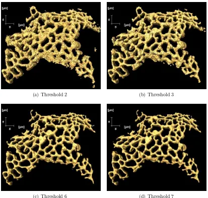
7.6 Effect of the threshold values on the size of the isosurface . . . 118

7.7 Box plots showing the effects of the threshold value T on the final of solid ER surface and volume values . . . 119

7.8 Edge lengthLe vs. smoothing applied to the sample of Figure 7.1 on page 112 . . . 120

7.9 The result of the skeletonisation process is a thin, median, structure which have the same homotopy type as the original object. . . 120

7.10 A graph representation of the solid ER . . . 121

7.11 Steps followed to obtain a graph from ER images . . . 123

7.12 Average edge diameter vs. distance to the nucleus and the corre-sponding Friedman test plot . . . 124

7.13 Edge length vs. distance to the nucleus and the corresponding Fried-man test . . . 125

7.14 Edge surface area vs. distance to the nucleus and the corresponding Friedman test . . . 126

7.15 Edge volume vs. distance to the nucleus and the corresponding Fried-man test . . . 126

7.16 Cropped regions of cortical plant ER near the cell wall, samples 1 to 4 . . 128

7.17 The solid ER network of different samples ((1) - (4)) is represented in each case as an undirected weighted graph G with weights representing the length of edges. The integers in the nodes are an arbitrary ordering of the vertices (nodes). . . 129

7.18 Cropped regions of the plant ER starting from the nucleus and extending out to the cell wall samples 1 to 4 . . . 130

8.1 An illustration of the movement of the ER. . . 137

8.2 Skeleton Assumptions. . . 138

8.3 An illustration of the dynamic ER pre-processing steps. . . 145

8.4 The steps followed to obtain the skeleton of the plant moving ER samples. . . 148

8.7 Types of junctions in the ER: end point, three way and four way

junctions. . . 153

8.8 An illustration of the plant ER loop closing. . . 156

8.9 An illustration of the ER loop opening. . . 157

8.10 Number of vertices vs time step . . . 159

8.11 Number of edges vs time step . . . 160

8.12 Average vertex degree vs time . . . 161

8.13 Total length in ROI vs time . . . 162

8.14 Total surface area in ROI vs time . . . 163

8.15 Surface area density vs time . . . 164

8.16 Volume-surface area ratio vs time . . . 165

List of Tables

1.1 An overview of the thesis . . . 5

7.1 Edge parameters . . . 127

7.2 Vertex parameters . . . 127

8.1 Junction (node) dynamic averages . . . 165

8.2 A summary of the dynamic ER analysis . . . 171

List of Algorithms

1 Distance Ordered Homotopic Thinning . . . 70 2 Chamfer map . . . 79 3 The average cross section diameter of a solid ER tubule. . . 101 4 Surface area of a solid ER branch . . . 102 5 Volume of a solid ER branch . . . 103

Nomenclature

α The aperture angle of a microscope objective; the angle under which light enters into the front lens of the objective, page 36

PH Pinhole; diaphragm of variable size arranged in the beam path to achieve optical sections, page 41

Ti Tumor inducing, page 22

4SED FOUR-point Sequential Euclidean Distance mapping, page 74

8SED EIGHT-point Sequential Euclidean Distance mapping, page 74

Airy disc The Airy disc refers to the inner, light circle (surrounded by alternating dark and light diffraction rings) of the diffraction pattern of a point light source. The diffraction discs of two adjacent object points overlap some or completely, thus limiting the spatial resolution capacity., page 38

Biosynthetic The biosynthetic route in the secretory pathway starts from the ER and ends at the plasma membrane, page 16

CER cortical ER, page 10

CLSM Confocal laser scanning microscopy, page 32

CM Confocal microscopy, page 31

Endocytosis The Endocytosis route in the secretory pathway starts from the plasma membrane to the trans-Golgi network (early endosome) followed by the Golgi or the pre-vacuolar compartment (late endosome) and lytic vacuole, page 16

ER The endoplasmic reticulum, page 7

FWHM Full width at half maximum of an intensity distribution, page 40

GFP Green fluorescent protein, page 8

G A graph: a set pair of a finite set of vertices and a finite set of edges, page 104

NA Numerical aperture of a microscope objective, page 36

NER The Nuclear ER, page 9

n refractive index of an immersion liquid, page 36

PER The peripheral ER, page 10

PMT Photomultiplier tube (detector used in CLSM): a light detector that multi-plies the signal, produced by the incident light, by large factors (as much as 100 million times) to enable weak signal, generated by limited flux of light, to be detected., page 34

PM The plasma membrane, page 15

PSF The intensity point spread function: a function which maps the intensity distribution of a point light source into the image space, page 39

PVC The pre-vacuolar compartment, page 16

QC Quality control, page 18

resel resolved element, page 46

SED Sequential Euclidean Distance mapping, page 74

SP The secretory pathway, page 15

Voxel a volume element, page 46

V The set of vertices in a graph, page 104

Part I

Background

1

Thesis road map

This thesis presents a collection of computational tools to help scientists study the form and movement of the endoplasmic reticulum, and other network-like structures, whose data were acquired and digitised by imaging equipment, such as a widefield or confocal microscope, and stored as digital images. The methods proposed are based on the representation of the network by its medial axis, or skeleton, which is then abstracted by a graph, that is a simple mathematical object, to simplify the analysis by exploiting well established graph theory algorithms.

The general workflow involves five main steps: (a) sample preparation and data acquisition (b) data pre-processing and noise removal (c) skeleton extraction (d)

4 Chapter 1. Thesis road map

motion analysis, and (e) data abstraction.

The overall text is organised into three major sections (see Table 1.1): Preliminar-ies, Main tasks, and Supplementary material. The Preliminaries section includes the title page, the abstract, the lists of figures, tables, programs, and algorithms, followed by the Nomenclature, and the Contents page.

The main tasks section consists of four parts: Background (Part I), Methodology (PartII), Results (Part III), and Conclusion (Part IV).

In addition to this introductory guide, PartIincludes Chapter2Motivations: which reviews the ER characteristics and highlights its main features, as well as the role it plays in the cell in general and in the secretory pathway in particular, with a focus on its geometric and dynamic characteristics, as reported in the literature, together with a brief description of the contemporary techniques utilised in its study.

Part II is a walk through of the steps followed to achieve the overall aim of this study. It thoroughly explains the procedure for collecting data (Chapter 3); the techniques used to remove noise and extract the skeletons and assign geometric parameters to their edges and vertices (Chapter4); the approach adopted to analyse the movement of the ER (Chapter5); and finally a brief review about Graph theory (Chapter6). Each of these chapters includes astate-of-the-art section which reviews the corresponding existing techniques.

PartIII is dedicated to Results and Discussion. It summarises the most important findings of this study and consists of two chapters: Chapter 7: The Static ER, and Chapter8: The Dynamic ER. Chapter7deals with the geometry of immobilised ER samples marked with a fluorescent protein and acquired by a confocal microscope. This chapter examines four geometric properties: the average length, the average surface area, and the average volume of a branch; as well as the average degree per junction. Chapter 8 extends the investigation further to include more realistic

5

ER samples by excluding immobilising agents from the above sample preparation protocol. This chapter adds to the four parameters introduced in the previous chapter, the average speed of a junction, the average moments of displacements of orderszero and two as well as the average maximum displacement per junction.

PartIV is the final part of this section. It concludes the work, highlights the main lessons learnt, and includes a view for future directions.

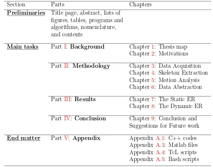
The last section consists of an appendix, a bibliography, and an index. The appendix includes all the codes developed throughout this study and consists of: Appendix A.1: C++ codes, Appendix A.3: Matlab files, Appendix A.4: TcL scripts, and Appendix A.5: Bash scripts.

Table 1.1: An overview of the thesis

Section Parts Chapters

Preliminaries Title page, abstract, lists of figures, tables, programs and algorithms, nomenclature, and contents

Main tasks Part I: Background Chapter 1: Thesis map Chapter 2: Motivations

Part II: Methodology Chapter 3: Data Acquisition Chapter 4: Skeleton Extraction Chapter 5: Motion Analysis Chapter 6: Data Abstraction

Part III: Results Chapter 7: The Static ER Chapter 8: The Dynamic ER

Part IV: Conclusion Chapter 9: Conclusion and Suggestions for Future work

End matter Part V: Appendix Appendix A.1: C++ codes Appendix A.3: Matlab files Appendix A.4: TcL scripts Appendix A.5: Bash scripts

2

Motivations

Eukaryotic cells contain sophisticated membrane-bound compartments that vary in shape and size. While the nucleus, lysosomes, and peroxisomes have almost spherical shapes; the endoplasmic reticulum (ER), Golgi apparatus, and mitochondria take the form of complex networks of sheets and tubules. Many of these organelles can be encountered in cells of different species in the same forms (seeStaehelin & Kang

(2008)). Among the largest and most complex of these organelles is the ER, which not only looks similar in different cell types; but, interestingly and intriguingly, also contains tubules and sheets with almost identical dimensions across cell types. Shape and size are therefore believed to play a major role in the function of the

8 Chapter 2. Motivations

ER (seeVoeltz & Prinz (2007)). This chapter exposes the most prominent features of the ER, focussing on its shape and size. It summarises the ER’s well known characteristics, and briefly describes the contemporary techniques commonly used in its study.

2.1

Introduction

The ER was initially described by EmilioVeratti(1902) in limb muscle of the water beetleHidrophilus liceusand muscle fibre from the fishCyprinus carpio. Porter et al.

(1945) later found the same lace-like structure in tissue culture cells by means of electron microscopy and consequently gave it the name of endoplasmic reticulum because of its network-like structure. A few years later, when comparing a vari-ety of cells in different species including avian fibroblasts, and macrophages; rabbit mesothelia, endothelia, and nephron epithelia; and rat glandular epithelia (parotid)

Palade & Porter (1954) found that the ER exists in all of these cell types. Ever since, the ER has become the focus of intense biochemical investigations to determine its role in living organisms.

The discovery of the green fluorescent protein (GFP), from the jellyfish Aequorea victoria, with which almost any protein can be tagged while retaining its function and dynamic properties(see Tsien (1998)), has revolutionised cell re-search. Both the ER’s lumen and membrane have been visualised using GFP. The former has been successfully visualised using soluble GFP fused to an N-terminal signal peptide and an ER retention signal (HDEL1_{) (see Boevinket al.(1999,1996)} and Boevink et al. (1998)); while the latter has been highlighted with a fusion be-tween Calnexin, a 67kD type-I membrane protein, and GFP (seeIronset al.(2003);

Kurupet al. (2005) and Runionset al. (2006)).

Combining GFP, and modern computer graphics algorithms, applied to data

ac-1

HDEL refers to: Histidine, Aspartic Acid, Alutamic Acid, Leucine

2.2 The ER visualised by confocal microscopy 9

quired by high resolution microscopes, has empowered cell research through im-proved cell visualisation. Not only has it become possible to obtain detailed micro scale 3D reconstructions of the ER; but it has also become possible to visualise the ER, and other compartments, from almost any arbitrary angle.

Depending on the resolution of the imaging equipment used, different subdomains of the ER can be differentiated.

2.2

The ER visualised by confocal microscopy

(a) Mammalian ER visualised by confocal mi-croscopy. Cytosolic ER takes a tubular con-nected network structure. Dimmer parts lie in out-of focus planes. Scale bar 10.00µm

(b) Plant ER visualised by confocal microscopy. The ER occupies a thin cortical region in plant cells. Regions that are in the focus plane are clearer than other regions. Scale bar 44.72µm

Figure 2.1: The ER visualised by confocal microscopy.

When visualised by confocal microscopy the ER looks like a 3D interconnected network of endomembranes that is organised in a complex system of tubules and cisternae. At this level of magnification, i.e. up to 200 nm lateral resolution, the ER is usually classified into either nuclear or peripheral according to whether it is in contact with the nucleus (seeVoeltz et al. (2002)). The nuclear ER (NER) is the

10 Chapter 2. Motivations

part of the ER that extends from the nucleus and contains a lumen surrounded by two sheets of membranes which are joined via the nuclear pores. The peripheral ER (PER), sometimes called cortical ER (CER), is the rest of the organelle and takes the form of a complex network that spreads out to the plasma membrane (Voeltz et al.,2002), to distribute proteins to different compartments in the cell, and enable communication with neighbouring cells via the plasmodesmata (Staehelin,

1997).

A region of interest (ROI) of the lower epidermis of an agroinfiltrated tobacco leaf is shown in Figure2.1(b)on page 9. GFP fused to an N-terminal signal peptide for entry into the ER and to a C-terminal ER retention signal that mediates retrieval from the Golgi apparatus to the ER (Anelli & Sitia,2007), when the protein escapes in the transport vesicles via bulk flow. The recombinant protein accumulates and highlights the ER which looks like a network that fills most of the cell volume. It is important to recognise that in confocal microscopy only the regions that are in the plane of focus will show the signal; so in order to obtain a 2D clear image of the ER it is sometimes necessary to scroll through the sample to find regions that completely lie in the plane of focus. This is what explains the presence of brighter regions compared to other regions in Figure2.1(a) on page9.

A confocal microscope is equipped with a detector (photomultiplier tube) or camera, which allows the recording of time series, that is indispensable for the study of the movement of the ER. The ER contains regions that appear to be fixed and relatively immobile as well as highly mobile regions that constantly remodel and appear to contain a dynamic flux of material. Fluorescence originates from soluble protein present in the lumen of the ER; so any apparent movement occurs through bulk ER remodeling.

Finally it is important to note that structures under the confocal microscope appear larger, because of the wavelength of visible light. The next section explains how the ER appears under an electron microscope.

2.3 The ER visualised by electron microscopy 11

2.3

The ER visualised by electron microscopy

Figure 2.2: The ER of notochord cells of Triturus alpestris. The ER extends in nearly parallel sheets. X 18,500, picture taken fromSelman & Jurand (1964). It is hard to see the tubular structure in the image. Scale bar 1µm.

When observed by transmission microscopy, i.e. up to 5nm resolution, the ER re-veals two distinct types: a rough type that is studded with ribosomes and known as Rough ER (RER); and a smooth type that is ribosomes free and known as smooth ER (SER). In mammals RER corresponds to the sheets and the SER to tubules (see Shibata et al. (2006)). In plants, SER is usually found in quantity in specialised cells.

The tubular network, observed using confocal microscopy, is virtually invisible un-der an electron microscope. It is difficult to see the network because it is not planar, and for EM very thin sections that might only include a few tubules in their entirety are imaged.

Figure2.2 on page 11illustrates what we can see using the EM and how difficult it is to see proteins in the lumen of the ER. It is possible to see a few regular arrays

12 Chapter 2. Motivations

of ribosomes which indicate the presence of the RER. The lumen is not as electron opaque as the cytosol; so we cannot really see a specific membrane. What we see in EM is actually a section through a sheet which represents rough ER studded with ribosomes. Tubular ER which appears to be more abundant in the cell and which fills most of the field of vision is harder to capture using EM. Finally, EM is much more time consuming and reveals much less than a confocal microscope but has the advantage of allowing smaller structures to be visualised.

Based on “ultrarapid freezing techniques”,Staehelin(1997), controversially, reports that the ER may be composed of more than sixteen discrete functional domains, each of which always contains the same family of proteins. However, it is important to note the connectivity of the ER; Voeltz et al. (2002) andPuhka et al.

(2007), report that when injected into the cell in an oil droplet, fluorescent dyes that cannot exchange between discontinuous membranes, diffuse throughout the ER; and the repeated bleaching of a region of the ER, whose lumen (or membrane) was tar-geted by a GFP-tagged protein, results in complete loss of fluorescence. These observations serve as evidence that the ER is a single connected compart-ment.

In mammals, the ER occupies more than 70% of the total area of the cell

(Fawcett, 1981) and over 10% of its total volume (Voeltz et al., 2002) and so is regarded as the largest single interconnected intracellular membrane sys-tem containing a common luminal space. In plants, cortical ER occupies a

very thin, almost two dimensional, layer of cytoplasm beneath the plasma

membrane, refer to Section 2.9 on page 20.

On the grounds of its dynamics, and for the purposes of this thesis, the ER is sub-divided into three essential parts, cytosolic, cortical, and nuclear ER. Cortical and nuclear ER are relatively immobile, whereas cytosolic ER is highly dynamic, which rapidly remodels itself in the form of tubular movements, where tubular structures appear or disappear in fractions of a second.

2.4 How the ER gets its form 13

The exceptional morphologic and dynamic heterogeneities of the ER are believed to be linked to its functional diversity (Verkhratsky,2007). The next section highlights the current understanding of how the ER gets its form.

2.4

How the ER gets its form

It is often easier to study the form of an object and relate it to its function rather than try to directly understand its function. Furthermore, not only do form, size, and other morphological properties differentiate and characterise living organisms, but they also reflect their optimal functions (Staehelin & Kang, 2008). How and why the ER gets its form has attracted the attention of many research groups. To identify the proteins responsible for shaping the ER,Voeltz et al.(2006), started by showing that vesicles purified fromXenopus laevis oocytes, coalesce to form tubu-lar networks. In the presence of GTP, they found that these networks could be stained with antibodies directed specifically against an ER marker.

They also found, usingmaleimide biotin, that sulphydryl reagents inhibited the for-mation of the network, and successfully identified Rtn4a/NogoA, a member of the reticulon family, as one of its targets. They then showed that the modification of

Rtn4a/NogoA, bymaleimide biotin, was correlated with the inhibition of the forma-tion of the network; and that antibodies againstRtn4a/NogoA suppressed network formation in vitro. More importantly, when over-expressing Rtn4a/NogoA, they found that it enhanced tubule formation.

Voeltz et al.discovered thatDP1, an integral membrane protein specific to the tubu-lar ER, interacts with Rtn4a/NogoA, while its homologue, YOP1, interacts with

Rtn1 and Rtn2, which areSaccharomyces cerevisiae reticulons. Furthermore, when deleting either YOP1, Rtn1 and Rtn2, or YOP1 and Rtn1 they obtained a abnor-mal tubular ER structure; which indicate thatYOP1 andRtn1 are what maintains the ER tubular structure.

14 Chapter 2. Motivations

Finally, when studying the topology of Rtn4 and YOP1, Voeltz et al. (2006) found that they both have larger hydrophobic regions (i.e transmembrane domains) than the average protein; between 30 and 35 residues instead of around 20 residues. This led to the conclusion that because of their conical topology, with their bases in the outer membrane surface, they maintain the ER tubular structure.

Rtn4a/NogoA belongs to the Reticulon family of ER resident proteins, which are restricted to the tubular ER. They collectively share a 200 amino acid region at their C-Terminal called “reticulon domain”, and are commonly attached to the ER by their hydrophobic C-terminal (Oertle et al.,2003). They occupy a larger area in the outer leaflet of a membrane than in the inner leaflet (seeVoeltz & Prinz(2007);

Voeltz et al. (2002) andVoeltz et al.(2006)).

In a later study,Voeltz & Prinz (2007) report four types of proteins responsible for the morphology of the ER: (a) the first type of protein stabilises the curvature of the ER membrane (b) the second type tethers the ER membrane to other cell com-partments (c) the third type regulates fission and fusion of the ER membrane (d) and the fourth type shapes the ER by stabilising certain morphologies.

The first type of proteins might use three possible mechanisms to generate a high curvature in the ER membrane, according to Voeltz & Prinz (2007); either (a) a protein scaffold bends the membrane, the reticulon family discussed above, or (b) the two leaflets of the bi-layer tend to stay together forcing certain morphologies or (c) the distribution of the lipids in the bi-layer is non-symmetric.

The second type of protein works by attaching the membrane of the ER to the cytoskeleton, another membrane, or to both (Voeltz & Prinz, 2007). For example, the attachment of the ER to actin filaments, in plants, causes it to take a tubular network structure and when depolymerised, the ER loses this structure.

The third type of proteins includes proteins p97 and V CIP135 which are thought to help the ER regain its shape after mitosis. They are believed to be regulated by phosphorylation or a post-translational modification during the cell cycle.

2.5 The ER and the Secretory Pathway 15

Finally, maintaining different domains, with the same shapes, in the ER is thought to be governed by three mechanisms: (a) selective diffusion (b) membrane tether-ing and (c) the segregation of membrane-shaptether-ing proteins into certain parts of the organelle, see Voeltz & Prinz (2007, and references therein).

The ER touches almost all other cell compartments (Staehelin,1997); because most of them require proteins that are initially translocated into the ER (Voeltz et al.,

2002); which explains the ER tubular network structure as an efficient means of distributing proteins to these compartments.

The size of the ER is important because the production of secretory proteins re-quires a large surface, hence the use of the ER membrane, which provides a larger surface than the plasma membrane (Vitale & Denecke, 1999). Understanding the form of the ER, therefore, provides valuable insight into its function. The next section summarises the importance of the ER in the secretory pathway.

2.5

The ER and the Secretory Pathway

An important point to raise here is that the ER is the entry point to the secretory pathway. It is the primary site of protein synthesis, maturation, and sorting, and plays a crucial role in protein folding, assembly and delivery of biologically active proteins to the proper target sites in the cell, its membranes and the extracellular space (seeNicchitta (2007); Schr¨oder & Kaufman(2005b) andSitia (2007)). These and other characteristics indicate the importance of understanding the function of this organelle.

To be transported from within the cell to the extracellular space, or backwards, biologically active proteins follow a well defined route known as the secretory path-way (SP). The forward route, known as biosynthesis route, starts with the ER, followed by the Golgi complex and the trans-Golgi network, before proteins reach the plasma membrane (PM) which surrounds the cell, and subsequently the extra

16 Chapter 2. Motivations

cellular space (Anelli & Sitia,2007). The reverse route, known as endocytosis, starts from the plasma membrane to the trans-Golgi network (early endosome) followed by the Golgi or the pre-vacuolar compartment (late endosome) and lytic vacuole. Although it is known that secretion occurs from the Golgi apparatus to the plasma membrane through carriers (Hawes & Satiat-Jeunemaitre, 2005), it is not currently clear which of these carriers is responsible for this task (see Hantonet al. (2005) and Denecke (2007)). The Golgi, the trans-Golgi, and the pre-vacuolar compart-ment (PVC), form cross junctions in both the Endocytosis and the biosynthetic routes.

2.6

The role of the ER in protein folding

The ER plays a crucial role in protein folding. Proteins are composed of both hydrophobic and hydrophilic domains. The exposure of the former is undesirable since it causes the formation of toxic aggregates that may be harmful to the cell. To prevent this from happening, proteins shelter the hydrophobic regions from the aqueous environment. The process of protein folding is usually accomplished by ER resident helper proteins called chaperones, which recognise, bind

and thus mask the hydrophobic regions.

In Eukaryotes, DNA is transcribed in the nucleus and mRNA transported through nuclear pores to the cytosol where it is translated by the ribosomes on the surface of the ER. This gives rise to a protein precursor which can then be targeted to other compartments in the cell (seeDenecke (2007) and Cooper(2000)).

Targeting mRNA to the ER is understood to be achieved in different steps. It starts with the synthesis of mRNA in the nucleus; which is then transported to the cytosol; where it is translated by ribosomes. Ribosomes on the surface of the rough ER start synthesising the nascent polypeptide chain. Secretory proteins synthesised on the RER usually have a signal recognised by the Signal Recognition Particle

2.6 The role of the ER in protein folding 17

(SRP), which recognises signal peptides as they emerge on the ribosome surface before they are fully synthesised. This is assisted by the SRP-receptor 2_{, which} guides the ribosome to the translocation pore, where translocation resumes. Proteins synthesised on the rough ER fold up with the help of a particular chaperone called the binding protein (BiP)3_{. BiP is also believed to close the translocation pores if} not occupied by ribosomes.

In addition to soluble proteins, the ER is also the site of synthesis of both types of membrane spanning proteins, part of which lies in the lumen and the other lies in the cytosol. In the case of Type I membrane spanning proteins, whose N-terminal lies in the luminal side of the ER membrane, translocation occurs as follows. First a signal peptide (SiP) is recognised and bound to the SRP. The complex is then transported to a translocation pore and translation continues. The protein is pulled through, possibly with the help of a chaperone. The portion of the protein lying in the transmembrane domain has yet to be translated. Translation carries on, but the transmembrane portion does not translocate further but remains inserted in the membrane. The ribosome will finish translating the mRNA and the remainder of the protein is exposed in the cytosol. Once the ribosome is disengaged from the mRNA, Type I membrane spanning protein remains associated with the translocation pore and the nascent chain as a portion exposed in the lumen and a portion exposed in the cytosol. The transmembrane domain will diffuse laterally out of the translocation pore into the membrane and will act as a membrane anchor (Denecke, 2007). Type II membrane spanning proteins, in which the C-terminal lies in the luminal side of the ER membrane, carry a transmembrane domain which acts as a signal for the entry into the ER. A large portion of the protein is synthesised in the cytosol before it is translocated into the ER. In some cases the transmembrane domain can be at the very C-terminus of the protein which means that the protein is fully

2

SRP-receptor recognises the SRP

3

BiP is a specialised protein which belongs to the heat shock 70 family, which has representatives in all compartments of the cell, where protein folding occurs, such as chloroplast, mitochondria, cytosol

18 Chapter 2. Motivations

synthesised before it can be translocated (Hanton et al., 2005), as in prokaryotes. This process is most likely assisted by chaperones on either side of the membrane (see Cooper (2000); Denecke (2007); Fawcett (1981); Vitale & Denecke (1999) and

daSilvaet al. (2004)).

Once properly folded, proteins exit the ER to the next destination in the SP, the Golgi apparatus, for further processing. Properly folded and synthesised soluble proteins reach the Golgi apparatus, from the ER, via transport vesicles. These proteins first enter the transport vesicles. The transport vesicles then travel, in turn, to the Golgi apparatus, where they fuse with its membrane and release the proteins in its lumen for further processing. This transport of vesicles occurs in both directions, ie from the ER to the Golgi (anterograde) and from the Golgi apparatus to the ER (retrograde by vesicle in plant cells, see Hawes & Satiat-Jeunemaitre

(2005) andCooper (2000)).

These vesicles are recycled to avoid continuous growth of the end locations of the secretory pathway, which can be detrimental (Denecke,2007). The fate of misfolded proteins is discussed in the next section.

2.7

The ER and quality control

It is not always guaranteed for proteins to fold up properly and reach their final, low energy, native conformation. This can be due to mutations or lack of partner pro-teins or cofactors. Their fate, in this case, is fundamentally different. Immature or misfolded proteins are retained inside the ER; they are unfolded for a second chance to properly fold; and if they fail to achieve this target, these aberrant proteins are targeted for final destruction or degradation. In addition to retaining immature or misfolded proteins, unfolding them or degrading them, the ER de-aggregates aggre-gated proteins. Protein folding is therefore closely related to the ER’s quality control (QC), a tight system, which ensures that the tasks of protein folding, modification

2.8 The ER and Golgi bodies 19

and assembly are properly performed (Anelli & Sitia, 2007).

Combined with ER-associated folding (ERAF) and transport vesicles, ER-associated degradation (ERAD) plays a major role in the export efficiency of certain cargo proteins Anelli & Sitia (2007); Wiseman et al. (200). ERAD involves many steps, according to Anelli & Sitia(2007): (a) first, misfolded proteins and terminally mis-folded proteins are discriminated by manose-trimming (b) They then, possibly, undergo partial unfolding and reduction, with the help of BiP and PDI, before retrotranslocation. (c) This is followed by dislocation, where Sec61, yeast Der1p and mammalian Derlin1, 2 and 3 are found to be involved (Anelli & Sitia, 2007), and (d) once they reach the cytosol they are ubiquitinated by E2-E3 complexes, then an N-glycanase removes the oligosaccharide moieties from glycoproteins, see

Anelli & Sitia(2007).

2.8

The ER and Golgi bodies

An interesting characteristic of the plant ER is the movement of Golgi bodies on the ER network (Hantonet al., 2005). The ER export sites and Golgi bodies move together as single secretory units (Hawes & Satiat-Jeunemaitre, 2005). ER export sites are specialised regions of the ER responsible for the formation of anterograde transport vesicles, which can be visualised using fluorescent protein fusions of GT-Pases or coat proteins that are responsible for COPII transport vesicles. It is im-portant to note that transport by vesicle in plants might not occur because of the possibility that Golgi bodies are associated with the ER. Little is known about the sites where the ER accepts retrograde transport vesicles. The so called ER import sites have yet to be visualised using specific markers (Denecke, 2007).

20 Chapter 2. Motivations

2.9

The plant ER

Plant cells offer a very attractive model for the study of the ER due to its pleiomor-phic nature (Staehelin, 1997), because in vegetative cells, whose volume is in large part occupied by the central vegetative vacuole, the ER is forced by turgour pressure against the plasma membrane and the cell wall. Therefore cortical ER occupies a very thin, almost two dimensional, layer of cytoplasm beneath the plasma mem-brane. This is ideal for the study of the ER architecture and dynamics using light microscopy. Once the realm of electron microscopy alone (Lichtscheidl & Hepler,

1996), the study of the plant ER has been recently revitalised by the use of fluores-cent protein reporters, which allow the study of ER dynamicsin vivo. The plant ER lumen has been successfully visualised using soluble GFP fused to an N-terminal sig-nal peptide and an ER retention sigsig-nal (HDEL) (seeBoevinket al.(1999,1996) and

Boevinket al.(1998)). Likewise, a fusion between calnexin and GFP (seeIronset al.

(2003); Kurupet al. (2005) and Runions et al. (2006)), has been used to highlight the plant ER membrane. The ER is highly dynamic and its constant remodelling depends on its attachment to underlying cytoskeletal structures. However, unlike the mammalian ER, the plant ER is not attached to microtubules but to actin filaments (Boevink et al., 1998). It is therefore predicted that specific myosin iso-forms mediate this interaction. Interestingly, when cells are treated with drugs like latrunculin that disrupt the cytoskeleton, ER movement is inhibited but its archi-tecture remains intact (see Boevinket al. (1998); Dreier & Rapoport (2000) and

Shibata et al. (2006)).

Drug inhibition studies have shown that whilst the streaming ER is dependent on actin, cortical network ER remodelling is dependent on the microtubules during the early stages of cell elongation. It has also been reported that oryzalin has an effect on ER dynamics in tobacco leaf epidermal cells, Arabidopsis roots and BY-2 cells but the effects were specific to the drug rather than microtubule depolymerisation

2.10 Common Techniques to study the ER 21

per se.(see Langhanset al. (2009)).

A shift to cisternal over tubular ER was proposed to occur due to an increased secre-tory load in differentiating maize root cap cells and during mobilisation of seed stor-age protein in germinating mung bean cotyledons (seeStephenson & Hawes(2005)).

2.10

Common Techniques to study the ER

As is the case for other organelles; studying the ER can be achieved through the de-livery of exogenous gene or protein material into the cell. A foreign protein, such as GFP-tagged protein, has to be expressed by the host cell for subsequent observation and analysis. Different methods, involving transient expression/stable transforma-tion, have been used to study the ER. These methods vary according to their speed and complexity. Among the most common of these are: electroporation, particle bombardment, andAgrobacterium-mediated transformation (see Hansen & Wright

(1999);Taylor & Fauquet (2002) and Balb´as(2004)).

2.10.1

Agrobacterium

-mediated transformation

Leaf infiltration with Agrobacterium (see Figure 2.3 on page 22) is a relatively easy technique that stably integrates DNA into the cell. Epidermal cells from infiltrated leaves can be analysed a few days after infiltration. Agrobacterium mediates the transfer of DNA to the genome of the plant. Transfection of it is quite efficient and the majority of the cells in the infiltrated area will start expressing recombinant proteins after two days. Small areas from infiltrated leaves can be taken as samples for analysis under the microscope (Sparkes et al., 2006).

Agrobacterium tumefaciens is an etiological agent for the plant crown gall disease, in which the gall comes from the transfer, integration, and expression of a set of

22 Chapter 2. Motivations

(a) Infiltration with a suspension of Agrobac-terium tumefaciens containing expression vector pVKH18En6-GFP-HDEL

(b) After 72h, sections from the infiltrated leaves were incubated in 1.0 µM latrunculin B for 30

min

Figure 2.3: Leaf infiltration with Agrobacterium.

genes called T-DNA. The genes in T-DNA can be replaced by any DNA sequence, which makesAgrobacterium tumefaciens ideal for gene transfer (Balb´as,2004). The genetic transformation starts by the transformation ofT-DNA4 _{fromAgrobacterium} tumefaciens to the host cell. T-DNA will then be integrated into the host cell’s genome. The introduced genes will finally be expressed in the transformed host cells.

After the induction of the Agrobacterium Vir protein machinery by phenolic com-pounds, theVirD1 and VirD2 proteins nick both borders at the bottom strand of the T-DNA. This gives a single-stranded T-DNA, which, together with several Vir

proteins, is exported into the host cell’s cytoplasm through a channel formed by

Agrobacterium VirD4 and virB proteins. The T-strand with one VirD2 molecule covalently attached to its 5’-end, which is the end of the T-strand which has the fifth carbon in the sugar-ring of the (deoxy)ribose at its terminus (Lodishet al.,

4

A discrete set of genes from Agrobacterium tumefaciens located on the tumor inducing (Ti) and delimited by a pair of 25-bp repeats; named left and right borders (Balb´as,2004)

2.11 Chapter Summary 23

2004), and coated with many VirE2 molecules forms a T-DNA transport complex. TheT-DNAcomplex is imported into the host cell’s nucleus with the help ofVirD2

andVirE2. Integration of the T-strand into the host cell’s genome is believed to be facilitated byVirD2 and VirE2 (Balb´as, 2004).

2.11

Chapter Summary

In conclusion the ER is an ordered connected membranous network that can be found in all eukaryotic cells; it is the port of entry into the secretory pathway; and is responsible for the synthesis, modification, assembly, proper folding or degradation, and the delivery of biologically active proteins to the proper target sites in the cell, its membranes, and the extra-cellular space (seeSchr¨oder & Kaufman (2005a) and

Schr¨oder & Kaufman(2005b)).

The form of the ER is conserved across eukaryotic cells, which stresses the im-portance of its role in the secretory pathway in particular and the cell in general (Voeltz & Prinz, 2007). This thesis considers three essential ER subdomains: nu-clear, nytosolic, and cortical ER, focussing on the cytosolic subdomain.

The form of the ER is believed to be controlled by four types of proteins: (a) the first type stabilises the curvature of the ER membrane (b) the second type tethers the membrane to other cell compartments (c) the third regulates fission and fusion of the ER membrane (d) and the fourth type shapes the ER by stabilising certain mor-phologies (seeVoeltz et al.(2002) andVoeltz & Prinz(2007)). Altogether, although considerable research has been devoted to understanding the role and functions of the ER, rather less effort has been paid to its geometric quantification despite the major role geometry plays in defining many of its functional attributes. The purpose of the remainder of this thesis is to develop a set of computational tools to help fill this gap.

Does the ER form change from one position of the cell to another? What are the

24 Chapter 2. Motivations

dynamic properties of the ER? Do they vary with location? Are they the same across different cell types? Do they change with different physical conditions? Is confocal microscopy appropriate to answer these questions and what are its limita-tions? The answer to these questions will lead to a more fundamental question; that is the relationship between the form and optimal function of the ER. GFP serves as an appropriate means of studying the ER,in vitro as well as in vivo; and taking advantage of the recent developments in computer graphics and confocal imaging, this thesis addresses the above questions by bringing together computer science, mathematics and biology, focussing on plant ER. As already stated in Chapter 1, this thesis presents a collection of computational tools to help scientists study the form and movement of the endoplasmic reticulum, and similar network-like struc-tures, whose data were acquired, digitised, and stored using a confocal microscope. The methods proposed are based on the representation of the reticulum by its skele-ton, which is abstracted by a graph, to simplify the analysis and exploit the well established graph theory algorithms. The following chapter highlights the protocol followed to prepare the samples, and the equipment used to acquire the data.

Part II

Methodology

3

Data Acquisition

After the overview of the ER in Chapter 2, this chapter takes a closer look at the origin of the data, and how it was obtained. It consists of two principal sections: (a) sample preparation -the leaf infiltration with Agrobacterium method; and (b) data acquisition to describe the equipment used in collecting the data, i.e. confocal laser scanning microscopy, reviewing the fundamental aspects of confocal microscopy, that are relevant to the overall aim of the thesis. Attention is paid to the resolution power of the equipment, as well as the main sources of noise and how it may affect the final results.

28 Chapter 3. Data Acquisition

3.1

Introduction

As is the case for other organelles in the cell, it is essential to find an appropriate, easy to handle model to study the form and movement of the ER using confocal microscopy. Vegetative cells offer a suitable model because of their pleiomorphic nature (Staehelin,1997). In this type of cell, the central vacuole occupies more than 90% of the overall volume of the cell (Marty, 1999; Reisen et al., 2005). Conse-quently, turgour pressure1 _{forces the ER against the plasma membrane and the cell} wall, which results in the flattening of the ER into a thin, almost two dimensional layer, making the plant ER a convenient candidate model with reduced geometric complexity; so instead of dealing with a 3D network, which can be considerably more complex to handle, the problem reduces to the analysis of a 2D network. It is already stated in Chapter 2, that studying the ER generally involves genetic transformation (DNA) and can be achieved in several ways. This thesis chooses the leaf infiltration with Agrobacterium method (see Figure 2.3 on page 22), because it is relatively fast, and highly efficient (Chen & Dubnau, 2004). Epidermal cells from infiltrated leaves can be analysed between two and five days after infiltration; in contrast to the three-month timescale of generating stable transgenic lines (see Section 2.10 on page21).

In our chosen method, Agrobacterium mediates the transfer of DNA into the genome of only a small region of the leaf. Furthermore, transfection is relatively efficient and most of the cells within the infiltrated area start expressing recombinant proteins within two to three days (Balb´as, 2004).

1

An outward force exerted by the plant cell’s content on its wall

3.2 Sample preparation 29

3.2

Sample preparation

Unless otherwise indicated, all calculations in the remainder of this study are re-lated toNicotiana tabacum cv Petit Havana, from which healthy, five to eight week old leaves grown in greenhouse conditions, were selected for agroinfiltration. Us-ing a syrUs-inge without a needle, these leaves were infiltrated with a suspension of

Agrobacterium tumefaciens (see Figure2.3(a) on page22 for clarification), which is a trans-kingdom DNA transfer capable plant pathogen, containing expression vector pVKH18En6-GFP-HDEL as described inBatoko et al.(2000).

The genetic transformation starts with the transformation of T-DNA from Agrobac-terium tumefaciens to the selected Nicotiana tabacum cv Petit Havana SR1 cells (Agrobacteria were at an OD6002 of 0.05). T-DNA was integrated into the host

cells’ genome; and the introduced genes were expressed in the transformed host cells (see Section2.10.1 on page 21 for details).

The following step in sample preparation depends on whether the aim is to study the static or dynamic ER. In the case of the latter (see Chapter8on page135), and after around 72h, the next step is to cut a small piece from an infiltrated leaf, mount it in water then observe it under the a confocal microscope (Leica TCS SP2 or Leica TCS SP5 in the case of this thesis, see Figure 3.1(a) on page 30and Figure 3.1(b) on page 30).

In the static ER case, and since we are dealing with optical z-sectioning, explained in section 3.3.1 page 31, it is altogether impossible, with the available microscopes, to obtain consistent z stacks without stopping the ER movement, due to its dynamic nature (see Section 2.1 on page 9).

For this reason, small pieces, about 1.0cm2_{, from the infiltrated leaves were cut, then}

incubated in 1.0µM Latrunculin B (Calbiochem, Nottingham, UK), for 30 min, to decelerate the movement of the ER (see Chapter 7), before they were mounted in

2

OD600refers to the optical density at 600nm, the measure of the amount of light absorbed by

the suspension of Agrobacteria.

30 Chapter 3. Data Acquisition

water and imaged using a Leica TCS SP5 confocal microscope (see Figure3.1(a)on page30).

(a) (b)

Figure 3.1: Two Leica microscopes were used in this study: (a) Leica TCS SP2: is used in the static ER analysis, (Leica, 2000) (b) Leica TCS SP5 (Leica, 2005) is used in the dynamic ER analysis. It can resolve structures as little as 200nm apart in the confocal plane and up to 400nm in the optical plane, and it is equipped with a galvo stage that provides fast z stacking with a stack as thick as 1.5mm (while Leica TCS SP2 can only image stacks up to 166µm (Leica,2005)).

3.3

Confocal microscopy

It is already known from Chapter 2 that an ER tubule is less than a micron in diameter, and is conserved across cell types (Voeltz et al., 2006). An appropriate high resolution microscope is therefore indispensable to study the form and move-ment of the ER. Despite being able to resolve structures in the region of 1nm, and thus surpassing other microscopy techniques; trans. electron microscopy TEM is inappropriate to study the geometry of the ER, because the latter is spread in three dimensional space; while EM requires thin, almost 2D sections (see Section 2.2 on page9). Furthermore, conventional widefield fluorescence microscopy images, whose

3.3 Confocal microscopy 31

z-dimensions are larger than the wave-optical depth, are commonly contaminated with light coming from out-of focus planes (Wilhelm et al., 2003), and thus require extra effort to obtain reliable results.

An alternative to both techniques is confocal microscopy (CM); because it has the advantage over both techniques not only by allowing one to image tubular ER; but also by enabling the microscopist to obtain improved resolutions, with high contrast optical sections, by restricting image information to thin, 0.5 to 1.5 µm, optical layers, through the specimen to obtain reduced out-of-focus artefacts, and improved signal-to-noise (SNR) ratios (Claxton et al., 2008).

Combined with an appropriate visualisation software such as Amira (Zuse, 2006), V olocity (Improvision, Waltham, MA),Imaris(BitPlane, Inc.), or similar software packages, the optical sectioning capability of CM has been exploited to derive 3D representations of different organelles, which can optically be sectioned through ar-bitrary angles.

This thesis uses the 3D representation of the ER to obtain its approximate geomet-ric, and dynamic properties, including: lengths of individual branches, their outer surface areas, their local diameters, and volumes; as well the average junction dis-placement, speed, acceleration, and moments of displacements (see Chapters7 and 8for details). The next section is a summary of the aspects of CM, that are relevant to the thesis.

3.3.1

An overview

CM, depicted in Figure 3.2 on page 32, was invented by Marvin Minsky in 1957 who, in order to visualise neurons in vivo, conceptually improved conventional light microscopy by introducing two novel ideas: (a) he placeda pinhole, at a position confocal with the point in the sample, to reject any light that has not origi-nated from the focal plane; and (b) rather than illuminating the entire plane of focus

32 Chapter 3. Data Acquisition

all at once, as in the case of conventional microscopy, Minsky sequentially illu-minated each point in turn; to avoid contamination with unwanted light spread as a result of illuminating the entire plane of focus (Paddock, 2001; Prasadet al.,

2007;Semwogerere & Weeks,2005).

To sum up Minsky’s design confocal microscopy is based on point illumina-tion and point detecillumina-tion; and its main advantage over conventional microscopy is the reduction of the out-of-focus glare originating from the scattered light coming from the planes above and below the plane of focus.

Arguably considered among the most notable advances in microscopy according to

Claxtonet al. (2008), Minsky’s invention still forms the basis of modern confocal laser scanning microscopy. Enhanced with modern optoelectronics, the discovery of the green fluorescent protein GFP, and the recent advances in computer graphics, it has a considerable impact on biological imaging. It is this combination that al-lows the derivation of 3D reconstructions of specimens, and permits one to obtain

Figure 3.2: The principle of CM. To produce an image element(pixel), the high intensity light of an appropriate wavelength reaches the specimen after hitting the dichroic mirror (left image). The excited specimen emits light of a different wavelength that passes through the dichroic mirror and the pinhole. The pinhole allows only light that has originated in the focal plane to reach the final destination, that is the PMT (middle image); light from other planes is rejected (left image). The PMT detects, and converts the signal (light) from analogue to digital via an AD converter. A computer stores the pixel information into a local memory. The system carries out the same procedure for all points in the current focal plane point-by-point, before it moves to the next plane; and repeats the same task. Once it scans the whole specimen the computer, with an appropriate software, can generate a 3D representation of the specimen. Figure taken from (Leica,2000)

3.3 Confocal microscopy 33

Figure 3.3: The principle of fluorescence: (1) the fluorophores are raised from their ground state, S0, to a higher unstable energy state S1′, (2) fluorophores lose part of the energy, in the form of heat, chemical reactions or through collisions with neighbour molecules, and consequently drop to an intermediate energy state, S1, (3) finally fluorophores drop to their initial, stable, ground state while emitting light of a larger wavelength, i.e. lower energy. Figure taken from (Leica,2005).

their arbitrary projections by producing stacks of sharp sections, restricted to thin focus planes, taken at different positions along the optical axiswithout physically damaging the specimen (Semwogerere & Weeks, 2005). CM may therefore be used to image both static (fixed) and dynamic (live) ER.

There are two CLSM imaging modes: (a) areflection modewhere light is reflected off the sample to produce an image, as in the case of the brain micro-vascular net-work (Fouardet al., 2006); and (b) a fluorescence mode: where fluorescence is stimulated from fluorophores3 _{applied to the sample. The former is usually used} to study the topography of the surface of tissues, while the latter mode is used in studying one, or more organelles by attaching multiple fluorophores to each one of them. What is common about the two modes is that they both rely on fluorescence to produce an image.

Figure3.3 on page33summarises the principles of the fluorescence mode, which are relevant to this thesis: (1) the applied high intensity light, or laser, of an appropri-ate wavelength λill (with the corresponding excitation energy Eill =hνill =hc/λill, where “ill” refers to illumination)4_{, raises the fluorophores (GFP), in the} speci-men from their ground, stable, energy state, denoted S0, to an unstable higher

3

A fluorophore is a fluorescent molecule

4

h= 6.62606896(33)×10−34Jsis Planck’s constant;c= 299,792,458m/sis the speed of light;

andνill is the frequency

34 Chapter 3. Data Acquisition

energy stateS′

1; part of the excitation energy dissipates, in the form of heat,

chem-ical reactions, or collisions with other molecules; causing (2) the fluorophores to pass to an intermediate state S1; finally (3) the fluorophores return to their

ini-tial stable state, after re-emitting light of a different colour having a lower energy Eem = hνem = hc/λem. The final image is formed from the emitted light as ex-plained in the next paragraph.

The formation of an image element (pixel) in CLSM can be summarised in the following steps (see Figure3.2 on page 32):

(i) the focused spot of light (laser with λill = 488nm in the current experi-mental settings) passes through the confocal pinhole (A), before it reaches the dichroic mirror, which reflects it towards the objective.

(ii) once it reaches the specimen, the laser illuminates asingle point in the focal plane for a short time (dwell time), just enough to stimulate fluorescence from the GFP applied to the specimen (between 5 to 50 µs(Stelzer, 2001)).

(iii) The stimulated GFP, fluoresces, as explained above, emitting light with a larger wavelength (λem = 507nm, i.e. lower energy, in the current experimental setting),

(iv) the emitted light passes through the objective, and is allowed to pass through the dichroic mirror, and finally pinhole (B) to reach its final destination that is the Photomultiplier (PMT) tubes, which detects it and passes it to an analogue-to-digital converter which transforms it into a pixel that is recorded by a computer,

(v) anXY scan controller (see Figure3.4on page35) directs the laser spot to scan the entire focal plane and build the corresponding 2D image. An appropriate

galvo stage moves the specimen sequentially to the next focal plane to form the next image,

3.3 Confocal microscopy 35

(vi) the entire 3D specimen is scanned in this fashion, and the series of images of the different focal planes (optical sections) is used to reconstruct the 3D specimen.

Figure 3.4: The main elements in CLSM. The main players in modern CLSM are: (a) the pinhole, which improves the resolution and the contrast of the final image (b) the PMT, which detects light passing across the pinhole (c) the excitation laser, or precisely its wavelength to cause the specimen to fluoresce (d) theXY scan controler to illuminate the focal plane point-by-point, (e) the z-control which controls the thickness of the focal sections and allows stacks of images to be obtained (f) the dichroic mirror that allows only the light reflected from the sample to reach the pinhole. Figure taken from (Wilhelm et al.,

2003).

In conclusion, the main optical elements that characterise a CLSM, that are relevant to this study, are: (a) the pinhole, featured by its diameter (Dph), and (b) the

objective characterised by its numerical aperture (NA), and magnification. Both of these elements are explained in the following sections.

3.3.2

The objective

The objective is a set of rotational symmetric optical lenses, which allow one to localise, focus, and magnify the specimen. Both light gathering and resolution

36 Chapter 3. Data Acquisition

Figure 3.5: The numerical aperture (NA) of a confocal microscope characterises its ob-jective and it depends on the index of refraction of the working medium (n) and the angle under which light enters the front lens of the microscope.

capacities of an objective depend on its numerical aperture (NA), which is a function of two parameters: the aperture angle (α), the angle under which light enters into the front lens of the objective, and the index of refractionn of the working medium (see Figure 3.5 on page 36); NA = n_·sinα (Leica, 2000). NA together with the wavelength of the excitation laser λill play a critical role in both lateral and axial resolutions that can be attained with CLSM as discussed in the following sections (Semwogerere & Weeks,2005, and references therein).

The magnification of an objective, denoted by Mo, is defined as the ratio between an object’s size and the image’s size; i.e. the factor by which the original size of the specimen is multiplied, to produce the final image; Mo = Si/Ss, where Si and Ss are the image size and specimen size respectively.

3.3 Confocal microscopy 37

Figure 3.6: The pinhole and the formation of a PSF: the pinhole is a spatial filter which prevents out-of-focus light reaching the PMT. It causes a point light source to appear as an Airy disc (top right), whose size depends on the numerical aperture of the front lens, the wavelength of the excitation light, the magnification of the objective, and the magnification factor of the optical system (Leica, 2000). The numerical aperture (N A) is a function of the index of refraction (n) of the working medium, and the angle under which light enters into the front lens of the microscope. The z-intensity vs distance from the optical axis profile takes the form of a bell (bottom left and top left), and the thickness of the optical section is defined by the full width half maximum (FWHM) of this profile.

3.3.3

The pinhole

The pinhole is a spatial filter whose main role is to reduce the amount of out-of-focus light, originating from the planes other than the focal plane, from reaching the PMT; and so to improve the contrast and resolution of the final image (Figure 3.6 on page 37).

Small pinhole diameters produce thin optical sections, better z-resolutions, but weak image signals; while large pinhole diameters degrade the confocal effect by produc-ing thicker optical sections, lower z-resolutions and stronger image signals (Pawley,

1995). Therefore, in addition to influencing the resolution, and the thickness of the