Compressive sensing in dynamic scenes

(1)

27-06-2017

MASTER THESIS

COMPRESSIVE SENSING

IN DYNAMIC SCENES

Nick Doornekamp

Faculty of Electrical Engineering, Mathematics and Computer Science (EEMCS)

Programme: Applied Mathematics

Chair: Hybrid Systems

Exam committee:

Prof.dr. A.A. Stoorvogel (UT)

Dr. M. Bocquel (UT/Thales)

Dr. P.K. Mandal (UT)

Dr. D.J. Bekers (TNO)

(2)

Abstract

(3)

Abbreviations and nomenclature

Abbreviations

CS Compressive Sensing BP Basis Pursuit

BPDN Basis Pursuit Denoising PF Particle Filter

SNR Signal-to-Noise ratio IC Information Criterion RC Rayleigh Cell

OSPA Optimal Subpattern Assignment YALL1 Your ALgorithms for L1 optimization FAR False Alarm Rate

HPFCS Hybrid combination of PF and CS SIR Sequential Importance Resampling

MC Monte Carlo

KLD Kullback-Leibler Distance

Nomenclature

f ∈Cn Original signal

Φ∈Cm×n Compression matrix

fc ∈Cm Compressed signal

Ψ∈Cn×n Basis

x∈Cn State vector recovered in CS framework

ˆ

x∈Cn Estimated state in the context of CS

A∈Cm×n Sensing matrix

ρ∈R Weighting parameter in BPDN

y∈Cm Noisy compressed signal (also measurement)

Niter∈N Number of YALL1 iterations

A(r)_∈

R Amplitude of componentr

ˆ

A(r)∈C Estimated amplitude and phase-shift of componentr

F(r)_∈

R Frequency of componentr

R∈_N Number of components

∈_R Stopping tolerance parameter in YALL1

N Support ofx

xNˆC Elements ofxoutside of the estimated support ˆN ωk ∈C Realization of the process noise at timestepk

σω Standard deviaton of the process noise

νk ∈C Realization of the measurement noise at timestep k

σν Standard deviaton of the measurement noise s State vector in the context of PF

(6)

1. Introduction

Compressive Sensing (CS) is a framework for the acquisition and processing of signals that are (ap-proximately) sparse when expressed in a suitable basis. That is, when the signal is expressed in this basis only a few of the coefficients of its expansion are not (approximately) zero. This assumption holds for many signals encountered in practice and many classical compression techniques also rely on this. The classical approach to signal acquisition is to sample the signal at the Nyquist rate, which is guaranteed to be sufficient for a complete representation of the signal. However, in many situations a complete representation is not necessary. Instead, a compressed version of the signal is used, which is much smaller than the Nyquist-sampled data in many situations.

For example, when a picture is taken with a digital camera, dozens of megabytes of data are collected. However, it turns out that when this image is transformed to e.g. the wavelet domain (as is done by the well-known JPEG1 compression method) only a relatively small number of wavelet coefficients are large; the others are approximately zero. In other words: much of the information can be captured using a small number of wavelets. Mathematically speaking, the image is approximately sparse in the wavelet domain. As a result, only the large coefficients have to be saved, while the quality of the image reconstructed from these coefficients is still close to the original. While this is useful, it also raises the question whether it is truly necessary to sample at a high rate if only a small amount of this data ends up being used in the final representation. With the CS framework the answer to this question is ‘no’: with CS, signals that are sparse in some domain can be recovered from a number of measurements that is small compared to what the Nyquist rate suggests. Instead of sampling the original signal directly, only a compressed version of it is acquired.

1.1 The CS framework

In the CS framework, the compressed signal is a linear function of the original signalf ∈_Cn_{. The}

compressed signal,fc∈Cm, can therefore be expressed as the product off and a matrix Φ∈Cm×n:

fc = Φf. We will refer to Φ as the compression matrix. Given the compressed signal the CS

frame-work recovers the state x ∈ Cn, which is related to the original signal through basis Ψ ∈ Cn×n:

f = Ψx. E.g. if Ψ is the Fourier basis, thenxcontains the Fourier coefficients off. In that case, if

f is the sum of a few sine functions, only a few elements ofxneed to be nonzero: xis sparse.

With the CS framework it is possible to obtainf by first solvingxfrom

ΦΨx=fc, (1.1)

and then computingf = Ψx. Whether this is actually done depends on the situation: in the context of this report it is not necessary to reconstruct f. Instead, the desired information is extracted from xdirectly. In the example where Ψ is the Fourier basis and f the sum of a few sines, this means the following: Instead of samplingf at or above the Nyquist rate, in the CS framework one would acquire only fc. By solving ΦΨx = fc for x, the x that underlies the original signal f is

(7)

obtained. With thisx, it would be easy to obtainf. If instead of obtainingf the goal is for example to determine which frequencies the sines in f have, this is not necessary: this information can be extracted fromxdirectly. In some areas, when the CS framework is applied without reconstructing

f, this technique is referred to as sparse sensing instead of CS.

In the following we will denote the product of the compression matrix Φ and basis Ψ asA∈_Cm×n

and refer to it as the sensing matrix. The CS framework is particularly interesting whenmis much smaller than n. That is, the dimension of the acquired measurement is much smaller than the dimension of the original signal. In that case, denotedm n, the sensing matrix will have many more columns than rows. Therefore system (1.1) is underdetermined, i.e. it has infinitely many solutions. Therefore, the key to CS lies in finding the right x from the under-determined system (1.1). Since the solution is assumed to be sparse, one way to proceed would be to select the sparsest solution that satisfies (1.1). This problem can be formalized as

ˆ

x= argmin

x∈Cn

{kxk0 s.t. Ax=fc}, (1.2)

wherekxk0denotes the number of nonzero elements inx. In words, this problem is the minimization

of the number of nonzero elements in x that can still describe fc perfectly. This problem is

com-binatorial, since each combination of nonzero positions in the solution vector has to be considered, which makes finding its solution intractable. However, it has been proven that the`0_-norm2_{in (1.2)}

can be replaced by the`1_{-norm in the sense that (1.2) and}

ˆ

x= argmin

x∈Cn

{kxk1 s.t. Ax=fc} (1.3)

have the same solution under certain conditions. For details on these conditions, the reader is re-ferred to the work of Cand`eset al. [10] or the work of Donoho [13]. In other words: the solution to (1.3) can be used to recover sparse vectors from (1.1). This is one of the fundamental results of CS. After all, since (1.3) is a convex problem, it is generally much easier to solve than (1.2). While solving such a problem for large inputs can still be expensive, much is known about how to do so and many efficient solvers are available. The problem in (1.3) is often referred to as Basis Pursuit (BP).

By demanding that Ax = fc it assumes noiseless measurements. If this assumption does not

hold (i.e. y= Φ(f+ν), where ν denotes the measurement noise) Basis Pursuit Denoising (BPDN) is more appropriate:

ˆ

x= argmin

x∈Cn

{kxk1+

1

2ρkAx−yk

2

2}. (1.4)

This problem can be interpreted as a trade-off between sparsity (first term) and signal fidelity (sec-ond term), where the relative weights of these two objectives is determined byρ.

Without any prior knowledge or assumptions about the signal of interest, classical signal pro-cessing theory like the Shannon-Nyquist theorem only guarantees perfect recovery when the number of measurements is more than twice the maximum frequency. Naturally, when prior information is available, as is the case with CS, this bound is pessimistic. In particular, it is shown that the number of compressive measurements m that is required to recoverxperfectly in BP (1.3) is proportional toS log(n), whereSdenotes the number of nonzero entries ofx. For the case of BPDN a bound on the reconstruction error (i.e. kx−xˆk) can be provided. Again, for details of this proof and other theoretical results we refer to [10] and [13].

2_{Note that even though the notation suggests otherwise,}_{k · k}

(8)

Applications for CS can be found in many areas. For example, Friedlanderet al. [17] apply CS to reconstruct the original audio from compressive measurements. CS can also be applied to (radar-) estimation problems, such the work by Bekers et al. [4], who apply CS to determine the Direction Of Arrival of a single target. In this report we will consider only estimation problems: estimating certain parameter that underlie the measured signal.

However, most of the research into CS focuses on application in the area of imaging. A promi-nent example is magnetic resonance imaging (MRI), where the number of measurements required for such a scan, and therefore the amount of time a patient has to spend lying as still as possible, can be reduced by CS. An introduction to CS applied to MRI is provided by Lustig et al. [14]. Another interesting application of CS is the single-pixel camera project of Rice University. This project shows that useful (recognizable) images can be acquired with very limited hardware and a number of papers have been published on this topic, such as the work of Duarteet al. [16].

1.2 Dynamic CS

The CS theory and applications that have been discussed so far all consider static scenes. Mea-surements are collected once to estimatex or reconstructf once. However, in many situations of interest the statexmight change over time: a dynamic scene. The simplest way to deal with such a situation is to take a snapshot at certain points in time and treat these snapshots as if they were static scenes. But it is clear that there is something to gain if information could be compounded over time. Therefore, we ask ourselves:

How can we make use of CS in dynamic scenes?

One of the tasks that might come with a dynamic scene is the tracking of targets, which is the task that is considered in this report.

An existing and versatile solution for the problem of tracking targets is offered by Bayesian fil-ters, such as the Kalman filter and the Particle filter (PF). PFs are known to be optimal3 _{from a}

Bayesian perspective as the number of particles tends to infinity, as is also described later in this report. However, one usually needs a large numbers of particles to make the numerical approxima-tion of a PF satisfactory, so that it requires a lot of computaapproxima-tional resources.

We will explore two approaches to make use of CS in a dynamic scene. The first is a ‘CS-only’ approach, which aims to use information from the previous timestep to speed up or improve the accuracy of the CS algorithm at the current timestep. We will refer to such ‘CS-only’ solutions as Dynamic CS. The second approach is to combine CS with a Bayesian filtering algorithm, or more specifically: a PF. The choice for the PF is motivated by its asymptotic optimality for a very general class of situations. The following two sections introduce Dynamic CS and the combination of CS with Bayesian filters, after which an overview of the rest of the report is presented.

The intuition behind Dynamic CS is that the outcome of the algorithm at the previous timestep can help the algorithm at the current timestep. This could be interpreted as providing the CS algorithm with prior information, where the prior information was gathered during the previous timesteps. In this section we describe a number of ways to incorporate prior information into the CS framework. Once we can make use of prior information the introduction of Dynamic CS is a

3_{By ‘optimal’ we here mean that the estimated posterior distribution is as close to the truth as possible (i.e. no}

(9)

matter of introducing a time-index.

One way to incorporate prior information into the CS framework is described in the work of Vaswani and lu [40]. They assume prior information on the support is available, where the support is defined as the positions wherexis nonzero or above a certain threshold in the cases of sparse and approximately sparse states respectively. The support is denotedN ={i|xi > α}, where α= 0 in

the case of a sparse state. In other words, they assume that some of the possible target locations are in fact known target locations.

In the following, we always regard a situation with noisy measurements4_{. The prior information}

about the support of, in the form of an estimated support ˆN, is introduced into BPDN by slightly changing the problem:

ˆ

x= argmin

x∈Cn

{kx_NˆCk1+

1

2ρkAx−yk

2

2} (1.5)

Here xNˆC is used to denote the elements of x outside the estimated support ˆN. Considering the `1-norm is used as a substitute for the `0-norm, this can be interpreted as follows: the number of nonzero elementsoutside of areas where nonzero elements were found earlier is penalized, instead of the number of nonzero elements in general. Vaswani and Lu [40] refer to the version of this problem without noise as Modified-CS or simply Mod-CS. Therefore (1.5) is referred to as Mod-BPDN. As noted by Friedlander et al. [17], the problem of sparse signal recovery with knowledge about the support was introduced in at least three papers: von Borries et al. [8], Vaswani and Lu [40] and Khajehnejad et al. [22]. All three make use of a weighted `1_{-norm to incorporate the support}

knowledge into the optimization problem. This norm is defined as:

kxk1,w =

X

i

wi|xi|, (1.6)

where wi is the weight of entry i of the support. Vaswani and Lu [40] and von Borries et al. [8]

set the weights of the estimated support entries to zero while the rest of the weights are one. Kha-jehnejadet al. [22] and Friedlanderet al. [17] propose a slightly more general approach, where the weights of the estimated support entries are allowed to be nonzero. Both do require that there are at most two different groups of weights, so all weights are eithera∈[0,∞) orb∈[0,∞).

CS algorithms that use prior information can be adapted to be dynamic by using the outcome of the previous timestep as the prior information of the current one. For example, Lu and Vaswani [26] describe ‘Dynamic Mod-BPDN’, where the Mod-BPDN problem is solved with the support estimated in the previous time-step.

ˆ

xt= min xt∈Cn

{k(xt)_NˆC t−1

k1+

1

2ρkAxt−ytk

2

2} where Nˆt−1={i|xˆt−1> α}. (1.7)

We will refer to (1.7) as Dynamic Mod-BPDN and CS algorithms that use information from the previous timestep(s) in general as Dynamic CS.

1.3 CS combined with Bayesian filters

Instead of trying to transfer information between pulses using only CS as in the previous section, another possibility is to deal with the dynamics of the scene with a Bayesian filter and let CS assist in some other way. In this section, a number of methods from the literature that use this approach

4_{To obtain an expression for the situation without noise, the term} 1

2ρkAx−yk

2

2 is replaced by Ax = y as a

(10)

are discussed.

Ohlssonet al. [32] consider a situation where neither the measurement equation nor the dynamic model is required to be linear. Since the CS framework described earlier this chapter requires the measurement equation to be linear, Nonlinear Compressive Sensing (NLCS) - see e.g. [5] - is used in this situation. Nonlinear CS is combined with a particle filter, resulting in what they call the Nonlinear Compressive Particle Filter (NCPF). They show that the combination is necessary in their testcase, since (nonlinear) CS alone does not take the temporal relationship between measurements into account and their implementation of PF alone performs poorly due to the high state dimension. The combination they propose is a particle filter with a fixed cardinality that can be updated through Nonlinear CS. By default the particle filter with fixed cardinality is used at each timestep. If the like-lihood of the signal estimated by this particle filter falls below a threshold, indicating that elements outside the currently assumed support are nonzero (i.e. there is a mismatch between the support used by the particle filter), the CS algorithm is used to detect which elements should be added to the support. Elements are removed from the current support when they fall below a threshold for a number of time steps. The idea of a PF with fixed cardinality that is updated through CS will be explored in section 4 and was implemented and tested during this project.

Ning et al. [30] combine a PF with CS for a Direction of Arrival problem where the targets are assumed to be on a grid. They use a CS algorithm to determine the initial locations of the targets and use this to create the (Gaussian) initial distribution for a PF. The idea of using CS to initialize a PF is discussed in section B.

Particle Filtered Modified Compressive Sensing (PaFiMoCS) by Daset al. [12] aims to deal with situations where the support does not necessarily change slowly over time, but does evolve according to a dynamic model. It does so by using a particle filter based on a dynamic model to provide the Mod-CS algorithm with a number of ‘close enough’ support-guesses (particles), sampled from the dynamic model. For each of these guesses the Mod-CS problem is solved to obtain an estimate of the signal value. They show that the PaFiMoCS performs better than a PF alone, single-snapshot CS at every timestep and Mod-CS alone. However, they do not consider the computational resources, which can be expected to be much higher for PaFiMoCS than for any of the other methods con-sidered: Clearly solving the Mod-CS optimization problem for each of the PaFiMoCS particles will take much more computational resources than solving only the Mod-CS problem once or running a basic PF with the same number of particles.

1.4 Research goal and contributions

The goal of this research is to explore ways to make use of CS in dynamic scenes. Clearly there are many possible tasks in dynamic scenes where CS could be of use, but in this report we consider the task of tracking multiple targets. We discuss two approaches that use CS to perform this task: Dynamic CS and a combination of CS and a PF. For both approaches we propose adaptions of the algorithms described in the literature to make them more suitable for the situation that we consider.

(11)

including their use of computational resources.

(12)

2. Simulation description

To make the methods comprehensible we first describe the situation to which they are applied. In the situation that we consider, at each timestep a signal pulse is generated. This pulse is the sum of an unknown number of frequency components. In section 2.1 this signal, denoted yk at time k,

is described in more detail. The objective of each of the methods is to determine an estimate of the state (which we will denote ˆsk) of the system: the number of components, their amplitudes,

and their frequencies. Finally these estimates are evaluated by a number of performance measures, which are described in section 2.2. These steps are illustrated by figure 2.1.

Signal generation

Method 1

Method 2

Method N

Performance evaluation

yk

ˆ

sk

ˆ

sk

ˆ

sk

[image:12.612.144.474.535.642.2]

. . .

Figure 2.1: Schematic overview of the simulation

2.1 Signal description

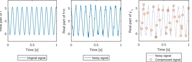
The original signal f that is considered in this report is a sum of complex exponentials. Noise is added to f before it is compressed to obtain the compressed signal y. We will consider only compression matrices Φ whose rows are a subset of the rows of an identity matrix. So to obtain the compressed signal from the noisy signal,m of thenmeasurements in the noisy signal are selected. This signal generation is illustrated by figure 2.2.

0 0.5 1

Time [s] -5

0 5

Real part of f

Original signal

0 0.5 1

Time [s] -5

0 5

Real part of f+n

Noisy signal

0 0.5 1

Time [s] -5

0 5

Real part of y

n

Noisy signal Compressed signal

Figure 2.2: An illustration of the original, noisy and compressed signal consisting of a single frequency component

(13)

in this report also have an imaginary part.

A single pulse is described by the following expression:

y= Φ

R

X

r=1

A(r)e2πiF(r)t+iξ(r)+n

!

, where n∼ CN(0, σ2). (2.1)

HereRdenotes the number of components and each componentrhas amplitudeA(r)∈R, frequency

F(r)∈Rand phase-shiftξ(r)∈[0,2π]. The estimated amplitude is complex, so that it contains both

the real amplitude and the phase shift. The notationCN(0, σ2) is used to denote a complex Gaussian distribution with mean 0 and varianceσ2_{. The term 2}_πF(r)_t₊_iξ(r)_{will be referred to as the phase.}

When a series of pulses is considered, a time-index will be added. The amplitude, frequency, and phase-shift of component rof pulsekare then denoted A(_kr),F_k(r), andξ(_kr), respectively. Unless it is necessary, the indexkwill dropped to improve readability. Throughout this report, ‘component’ and ‘target’ are used interchangeably and a timestep this refers to the index k. In the context of radar, what is referred to as a timestep or pulse in this report, is referred to as ‘slow time’. The time within a pulse is then referred to as ‘fast time’. In this report such a distinction is not necessary; a timestep refers to ‘slow time’.

In this report, σ = 1 and the amplitudes of the components are determined by the specified Signal to Noise Ratio (SNR). The SNR is defined as the ratio between the power of the signal and the power of the noise. The SNR is usually denoted in dB. The amplitude A of a signal with an SNR ofxdB is then

√

σ2_·₁₀10x.

The PF and the CS algorithms that are compared and combined in this report make use of the same input signal. To be able to compare them, they have to generate outputs that essentially contain the same information. Buts described in section 4.1.3, a PF will have an estimated posterior density as its output, while CS provides a single point estimate. Therefore, we extract a point estimate from the estimated posterior and determine the performance of the PF based on this point estimate.

This point estimate of the state contains the amplitudes and frequencies of the estimated components: ˆ

s= [A(1)_F(1)_...A(R)_F(R)_{]. The output ˆ}_x_{of the CS algorithms are related to the grid that is used,}

which could be interpreted as a number of frequency bins. For example, when a grid between 0.5 Hz and 10.5 Hz with a grid cell of 1 Hz is used, the information ‘one component with amplitude 1.5 and frequency 5 Hz, one component with amplitude1 _{2.5 and frequency 7 Hz, both with}

phase-shift zero’, would be presented as ˆx = [0 0 0 0 1.5 + 0i 0 2.5 + 0i 0 0 0] in the output of CS. In words that is a response of 1.5 in the frequency bin 4.5 Hz-5.5 Hz and a response of 2.5 in the frequency bin 6.5 Hz - 7.5 Hz. The same information would be in the point estimate of the PF as ˆ

s= [1.5 + 0i, 5, 2.5 + 0i, 7]. In section 3.1.3 the conversion of ˆxto the format of ˆsis discussed. During the internship that preceded this graduation project [15]2 the idea of running a PF on compressive measurements was explored. One of the challenges when working with compressive mea-surements is dealing with the correlations between meamea-surements that the compression can cause. Note that it depends on the type of compression whether correlations are introduced at all. An example of a type of compression that introduces correlations is one that sums the signal values over an interval to obtain a compressed measurement. When two compressed measurements have overlapping intervals, they will be correlated. In [15] two methods of dealing with these correlations are investigated: updating the covariance matrix to include these correlations and using a prewhiten-ing transformation.The latter transforms the noisy signaly so that it has uncorrelated noise again.

1_{In practical situations, the amplitude will have a unit. In a radar use-case this could be Volt, for example.}

However, since we assume the noise level to be known (see also 5.4.1), we will divide any signal by this noise level so that the noise level of the signal becomes one (dimensionless). Therefore we will not denote any unit for amplitude in this report.

(14)

This is useful since, when applying CS methods, one often assumes uncorrelated measurement noise. While this is not necessary for running a CS algorithm, it is a common assumption in the deriva-tion of many recovery guarantees. In this report we will use only types of compression that do not introduce correlations. As mentioned earlier, we will consider compression matrices whose rows are a subset of the rows of an identity matrix.

2.1.1 Relation to a radar use-case

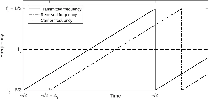
As a motivation for considering the signal described in equation (2.1), we relate this signal to the range estimation in Frequency Modulated Continuous Wave (FMCW) radar. In this type of radar, an on-going sequence of pulses with a linear phase is transmitted. That is, the transmitted frequency, denotedftransmit, linearly increases within each pulse. The difference between the highest and lowest

frequency in a pulse is the bandwidth, denoted B and the average frequency is referred to as the carrier frequency, denotedfc. The duration of a pulse is denotedτ. The signal that is received after

it is reflected by an object is the same, only delayed by ∆t. This is is illustrated by figure 2.3.

- /2 - /2 + _t Time /2

f_c - B/2 f_c f_c + B/2

Frequency

[image:14.612.120.489.280.453.2]

Transmitted frequency Received frequency Carrier frequency

Figure 2.3: An illustration of the transmitted and received frequencies in an FMCW radar

ftransmit(t) =fc+ B

τt where − τ

2 < t <

τ

2. (2.2)

Consequently, the phase of the transmitted signal, denotedφtransmit, is quadratic over time:

φ(t) = 2π

Z

ftransmit(t)dt= 2πfct+π B

τt

2_. _(2.3)

That is, the phase at timetis the integral of frequency times 2π. Therefore the transmitted signal

stransmitis

stransmit(t) =a·e2πifct+πi

B τt

2

. (2.4)

This transmitted signal travels through the air until it is reflected by an object. Provided this object is stationary, the signal received by the radar receiver is then

sreceive(t) =a0·e2πifc(t−∆t)+πi

B

τ(t−∆t)2_. _(2.5)

(15)

travels at speedc- usually the speed of light in a radar context - then ∆t=2_cr. For the purpose of

this section, the value ofa0 is not important, but in practice it is given by the radar equation, which can be found in any introduction to radar principles. If the goal is to determiner, the next step is to mix the two signals. This operation is defined for a pair of two signalss1 ands2 assmix=s∗2s1,

wheres∗₂is the complex conjugate ofs2. If the received signal is mixed with the transmitted signal,

we obtain what is referred to as the beat signal (denotedsbeat):

sbeat(t) =a00·e(2πifc(t−∆t)+πi

B

τ(t−∆t)2)−(2πifct+πiBτt

2

) =a00 e2πifc∆t+2πiB∆τtt−πi B(∆t)2

τ =a00·eφ(t)

(2.6) Now, all that is required to obtainris to determine the (constant) frequency of the beat signal:

fbeat(t) =

1 2π

dφ dt =

B∆t

τ =

B τ

2r

c . (2.7)

If there are multiple objects that reflect the transmitted wave, the received signal will be the sum of these signals. In that case, the beat signal contains multiple frequencies, which results in a signal of the form described in equation 2.1. There are other examples of relationships between the frequency of the beat signal and distance to a target or its velocity in other radar types, but these will not be discussed here.

2.1.2 Scenario

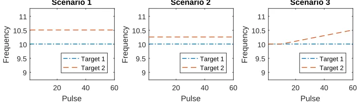
The considered algorithms will be applied in three scenarios, which are illustrated in figure 2.4.

20 40 60

Pulse 9 9.5 10 10.5 11 Frequency Scenario 1 Target 1 Target 2

20 40 60

[image:15.612.122.487.366.471.2]

Figure 2.4: A graphical representation of the two scenarios considered

Scenario 1 considers two targets at a distance (i.e. frequency difference) of 0.5 Hz from each other, in scenario 2 this distance is 0.25 Hz. This distance can be varied more to determine how far targets need to be apart before they are distinguished consistently by an algorithm. Then these scenarios could be used to determine the resolution as the smallest distance where the algorithm can distin-guish the two targets in at least a given fraction of the Monte Carlo (MC) runs.

(16)

difficult to distinguish them. So, the sooner an algorithm can distinguish the two targets, the better.

In all scenarios the amplitude and phase-shift from equation (2.1), and therefore the complex estimate that is estimated as well, are constant but not known to the algorithm.

2.2 Performance evaluation

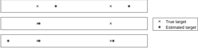
The state that is estimated by the different algorithms consists of an estimated number of targets and their locations. Since all of the numerical results in this report come from simulations, the ground truth is known and these estimates can be compared to that. Clearly, the closer the estimate is to the truth, the better the estimate. In a situation where there is always one true target and one estimate, defining what the distance between the estimate and the true target is, is fairly straightforward. However, since the true number of targets is not known a-priori, the estimated number of targets does not necessarily match the true number of targets. Therefore, in a situation where the number of targets is also estimated, the definition of the distance between the estimated state and the true state is not obvious. This is illustrated by figure 2.5: it is not intuitively clear which of the three estimated states is the ‘closest’ to the true state.

[image:16.612.137.470.301.382.2]

True target Estimated target

Figure 2.5: Different estimates of a situation with two true targets. Figure based on fig. 1 of [35]

In this section we first introduce the Rayleigh resolution criterion, which puts a handle on the maximum distance between a target and an estimate for which we still allow them to be associated to each other. After that, we discuss two approaches to measuring how close the estimated state is to the truth, which make use of this Rayleigh criterion. In the first a number of statistics such as the number of true targets that was correctly identified and the number of false alarms is considered. The second approach considers the distance between the estimated state and the true state to be a combination of the distance between the estimates and the true targets and the difference between the estimated number of targets and the true number of targets.

2.2.1 Rayleigh resolution criterion

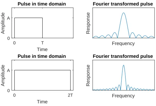
To declare whether a true target is found by the algorithm, one needs to specify how close an esti-mate needs to be to a true target in order to be associated to that target. For this purpose, we will make use of the Rayleigh cell (RC), which has its origins in optics. It is defined as the distance be-tween two point-sources of equal amplitude where the principal intensity maximum of one coincides with the first intensity minimum of the other [7]. When two true targets are at least one RC apart, they can be distinguished according to the Rayleigh resolution criterion. Therefore, it seems reason-able to relate the maximum distance where an estimate can be associated to a true target to this RC.

(17)

longer the pulse is, the narrower the principal peak of the Fourier transformed pulse is.

0 T

Time

0 A

Amplitude

Pulse in time domain

Frequency

Response

Fourier transformed pulse

0 2T

Time

0 A

Amplitude

Pulse in time domain

Frequency

Response

[image:17.612.175.431.111.285.2]

Fourier transformed pulse

Figure 2.6: Pulses with a constant frequency of different lengths and their Fourier transform

This width is important because when two components are close to each other in terms of frequency, their corresponding sinc-functions will overlap too much, as is illustrated by figure 2.7. There we see that components close to each other results in one large peak (rightmost plot) instead of two distinguishable peaks (leftmost plot). The principal peak of the sinc has its first zero at a distance of _T1 from the middle, so that the Rayleigh criterion is at _T1 as well. If the targets are further away we declare them to be resolved, if they are closer together they are declared unresolved.

Frequency

Response

Resolved

Frequency

Response

Rayleigh criterion

Frequency 1 Frequency 2

Frequency 1 + frequency 2

Frequency

Response

Unresolved

Figure 2.7: Sums of Fourier transformed pulses of different constant frequency components

2.2.2 Association of estimates to true targets

[image:17.612.102.511.408.566.2]

(18)

With the definition of the RC from the previous subsection, the following rules are applied for the association of estimated targets to true targets:

• Estimates further than half a RC away from the true target are not associated to this target. So each true target has a window around it with the width of a RC and only estimates inside that window can be associated to this target.

• At most one estimate can be associated to each target.

• Estimates that are outside all windows are considered to be false alarms.

• Estimates are associated to true targets in the way that has the smallest total Euclidean distance.

After the estimates have been associated to the true targets, a number of statistics can be extracted:

• Number of true targets that was found (i.e. have an estimate associated to it);

• Number of true targets missed;

• Number of false alarms;

• Number of estimates inside at least one window but not associated to a true target.

These four statistics together can provide an impression of the performance. Depending on the situation, one statistic might be more important than the other. When analyzing the ability of the algorithm to distinguish two targets, the number of targets missed largely determines the perfor-mance. However, an algorithm that consistently finds both targets but produces many false alarms and estimates not associated to a target, is undesirable in many practical situations. The relative importance of these statistics depend on the situation at hand.

An exhaustive search over all possible associations of estimates to true targets is performed. The result of this search is the set of associations which has the smallest total Euclidean distance of those where the maximum number of estimates is associated to a true target. This procedure is detailed by the examples in section 2.2.4.

2.2.3 Optimal Subpattern Assignment Metric

The statistics described in the previous subsection do not provide much information about the ac-curacy of the different methods. In a sense, acac-curacy is embedded in the requirement that estimates more than half a RC away from the target cannot be associated to that target, but this requirement does not distinguish between the estimate being close to the target or just barely within the RC around the target. To get a more complete picture of the performance of the different methods, an-other metric will be included in the analysis: The Optimal Subpattern Assignment (OSPA) metric, proposed by Schuhmacheret al. [35].

The OSPA metric considers both the accuracy of the estimated target locations and the estimated number of targets. It makes use of a distance between a given estimate and a given true target similar to the one in the previous subsection. They define the distance with cut-offcbetween two frequencies

F(j) and F(i) to bed(c)(F(j), F(i)) = min(c,kF(i)−F(j)k1). Then, given the vector of estimated

target locations ˆF = [ ˆF(1)_{, ...,}_F_ˆ(n)_{] and the vector of true target locations} _F _{= [}_F(1)_{, ..., F}(m)_{], the}

OSPA of orderpwith cut-offcis defined as

OSP A(_pc)(F,Fˆ) =







1

R

minπ∈ΠnΣ m

i=1d(c)( ˆF(π(i)), F(i)), cp(n−m)

_p m≤n

OSP A(pc)( ˆF , F) m > n

(2.8)

Here Πn is the set of permutations of {1,2, ..., n} and k · kp is the Lp-norm: k(x, y)kp =

(|x|p₊_|_y_|p₎1_p_{. The first term considers the sum of the ‘cut-off’-distances between the true}

(19)

the number of estimated targets. With this definition, c is the penalty that is given to estimates that are more thancaway from any of the true targets.

The parameterc is interpreted as the maximum distance between an estimate and a true target at which the estimate can be assigned to that target. As suggested at the start of this section, we will take this to be half a RC, i.e. c= ₂1_T. The order parameter pdetermines how sensitive the metric is to estimates far from any of the true targets. The higherp, the more sensitive the metric is to such estimates. Schuhmacheret al. suggest usingp= 2, which is what we will do here as well. An important advantage of takingp= 2 is that the association of targets within a RC of a true target in the previous subsection will correspond to the same pairs of estimates and true targets as the permutationπof minπ∈ΠnΣ

m

i=1d(c)( ˆF(π(i)), F(i)).

2.2.4 Examples

This subsection presents some examples that illustrate the procedure of associating estimates to true targets. It is recommended to look at these pictures in color rather than in grayscale.

10 10.3 10.7

Target 1 Window 1 Target 2 Window 2 Estimate

Figure 2.8: Two targets, one estimate

Figure 2.8 shows a situation where there are two true targets, but only one estimate. This estimate can be associated to both of the true targets, but will be associated to the closest true target: target 1 in this case. So in this case we have one missed target and one target found. The OSPA in this example is√0.32_{+ 0}_.₅2_≈₀_._58.

9.6 10 10.3 10.7

Target 1 Window 1 Target 2 Window 2 Estimate 1 Estimate 2

Figure 2.9: Two targets, two estimates

In figure 2.9 we have two estimates that are both inside at least one window. Since estimate 1 is outside the window of target 2 the distance between them is infinite by our definition. Therefore in the association with the smallest total distance estimate 2 is associated to estimate 1 while estimate 1 is associated to target 2, even though estimate 2 is closer to target 1 than to target 2. The OSPA in this example is√0.42_{+ 0}_.₄2_≈₀_.₅₇

(20)

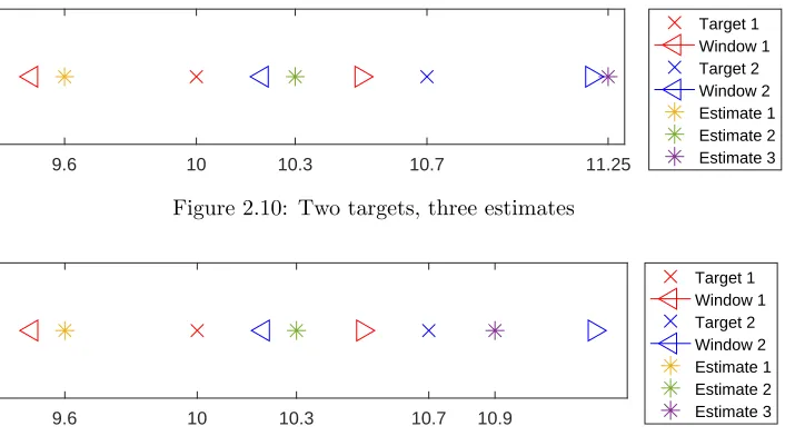
9.6 10 10.3 10.7 11.25

[image:20.612.138.491.74.270.2]

Target 1 Window 1 Target 2 Window 2 Estimate 1 Estimate 2 Estimate 3

Figure 2.10: Two targets, three estimates

9.6 10 10.3 10.7 10.9

Target 1 Window 1 Target 2 Window 2 Estimate 1 Estimate 2 Estimate 3

Figure 2.11: Two targets, three estimates

Figure 2.11 shows what happens if the third estimate is closer to target 2. In this case estimate 3 will be associated to target 2 and estimate 2 is associated to target 1. Estimate 1 cannot be associated to any of the targets, but since it is inside at least one window, it will not be classified as a false alarm. Such a situation might arise when one true target results in more than one estimate or in a cluttered scene where objects might be mistaken for targets. The OSPA in this example is

√

0.32_{+ 0}_.₂2_{+ 0}_.₅2_{= 0}_._62.

As a last example we consider the situation where two estimates are equally far from a true target: a tie. In the case of a tie, the entry that comes last in its row/column will be used. Since the vector will be ordered by frequency in the context of this report, this will be the one with the highest frequency. Ties might occur when grid-based methods like CS are used, while the probability of a tie is zero for methods like the PF, whose estimates can be anywhere in the continuous state space.

2.3 Algorithm efficiency

In many dynamic scenes it is not only of importance to obtain an accurate estimate of the state, but also to obtain it quickly. There is usually a trade-off between speed and accuracy. Both CS and a PF have parameters that can be changed to shift the balance between accuracy and computational re-sources, which are introduced in sections 3.1.2 and 4.1.1 respectively. If a better accuracy/resolution is desired, more computational resources will be required. These parameters can be tuned so that all algorithms have the same performance (e.g. in terms of ability to distinguish two targets), so that the amount of resources can be compared. This provides an answer to the question how efficient these algorithms are.

(21)

3. Dynamic Compressive Sensing

In this chapter we investigate different variants of Dynamic CS. These variants are based on the same optimization problem as static CS, namely BPDN (as discussed in section 1.1). As an introduction to the different variants, we first describe in section 3.1 the specific convex optimization algorithm that we will use to solve BPDN. The main section of this chapter is section 3.2, in which we discuss Dynamic CS and the proposed variants. In particular, the variants of the Dynamic Mod-BPDN algorithm described in the literature are proposed in sections 3.2.3 and 3.2.4. The difference between these variants is in how they make use of information from the previous timesteps. But they are all motivated by the idea that information from previous timesteps can help to speed up the optimization algorithm.

3.1 Optimization

In this subsection, we discuss algorithms that can be used to solve the (L1 relaxation) optimization problems such as the (variants of) BPDN from equations (1.4) and (1.7). The focus of this section is on the solver that will be used: YALL1. Besides the algorithm that this solver uses, we also discuss its most important parameters and how they are tuned for our purpose.

3.1.1 YALL1 algorithm

The solver that was used during this project is ‘Your ALgorithms for L1 optimization’ (YALL1) [42, 43], which is a Matlab solver that can be used to solve a variety of`1_{-minimization problems.}

The algorithm is grid-based in the sense that the estimated state always lie on a pre-specified grid. It is assumed that the measurements are a linear function of the underlying state plus uncorrelated Gaussian noise (i.e. y= Ψx+ν).

To solve the optimization problem efficiently it relies on the Alternating Direction Method (ADM). In the ADM, problems of the following form are considered:

min

x,y{F1(x) +F2(y)|Ax+By=b}. (3.1)

whereF1andF2are convex functions. The property of such problems that ADM exploits is that the

(22)

to y. And then finally, with the new values forxandy, also with respect toλ. A more elaborate description of the ADM applied to BPDN (equation (1.4)) can be found in the work of Yang and Zhang [41]. In this work, they also compare its performance to other`1_{-solvers, and conclude that}

YALL1 is “efficient and robust” and “competitive with other state-of-the-art algorithms” [41].

3.1.2 YALL1 parameters

Weight of signal fidelity

As mentioned in the introduction of this report, the problem that is solved by YALL1 in the context of this project - see equations (1.4) and (1.7) - aims to balance sparsity and signal fidelity. The relative importance of these two factors is determined by the parameter ρ, where the weight for signal fidelity is inversely proportional to ρ. A larger ρ means a smaller weight for signal fidelity and therefore a larger relative weight of sparsity. Therefore, the largerρ, the sparser the solution.

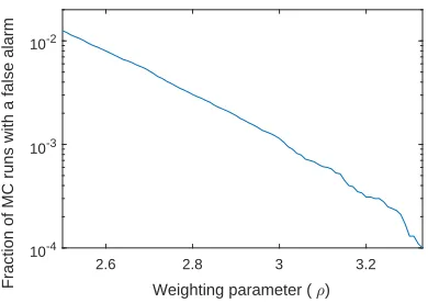
Since different values ofρusually lead to different solutions of the optimization problem, choosing a proper value forρis important. For the purpose of this project we will set ρbased on a noise-only simulation. In this simulation, a noise-only signal is fed into YALL1, for a range of values for ρ. For each of these values ofρthe fraction of MC runs where at least one target was found is used to approximate the false alarm rate (FAR) corresponding to thisρ.

2.6 2.8 3 3.2

Weighting parameter ( )

10-4 10-3 10-2

[image:22.612.210.405.320.458.2]

Fraction of MC runs with a false alarm

Figure 3.1: Fraction of MC runs with a false alarm for varyingρ

In this figure the ρcorresponding to the desired FAR can be found.

Table 3.1: ρ’s corresponding to given false alarm rates

Noise-only FAR 10−2 ₁₀−3 ₁₀−4

ρ 2.55 3.01 3.33

Stopping tolerance

The YALL1 algorithm has two stopping criteria, which are checked every two iterations. The first concerns the relative change:

kxi−xi−1k

kxi_k <(1−q). (3.2)

(23)

of three inequalities and all three have to be satisfied. The first of these concerns the same relative residual as equation (3.2):

kxi₋_xi−1_k

kxk <(1 +q) (3.3)

The other two concern the difference between the primal and dual solutions (referred to as the du-ality gap) and the size of the norm of the residual relative to the norm of the current estimate of the state (referred to as the relative residual). For more details we refer to the work of Yang and Zhang [41]. The choice ofaffects the number of iterations that are required to meet the stopping criterion, where a smallercorresponds to more iterations.

Without going into too much detail we also mention here the parameter γ, which determines the step length in the iterations of YALL1. By default it is set to 1, but that turned out to cause some problems with convergence in the context of this report. In previous work with YALL1, TNO experienced the same issues. These problems did not arise whenγ = 0.9, as was done during this project.

3.1.3 Post-processing

As mentioned in section 2.1 the output of YALL1 has a different way of presenting the information about the state than the PF. In particular, the output of YALL1 is related to a grid: the output corresponds to the intensity of the response for each of the grid-points. The post-processing proce-dure converts the YALL1 output to a format that can be compared to the point estimate produced by the PF. For on-grid targets this conversion is straightforward, since each nonzero corresponds to an estimated target. The only post-processing that is required is a low threshold to weed out nonzero elements caused by machine-accuracy issues. In this report we will only consider on-grid targets. The main reason for this assumption is the extra post-processing that will be needed for off-grid targets. This is illustrated by the figure below. In section 5.4 the case of off-grid targets is discussed in some more detail.

Frequency

Response

On-grid target

Frequency

Response

Off-grid target

Figure 3.2: An illustration of what the true response of on-grid and off-grid targets might look like

3.2 Dynamic CS

(24)

3.2.1 Initial condition

One way to provide prior information to CS is via its initial condition (i.e. the initial condition for YALL1). By default, the initial condition of YALL1 isx0=A∗y, whereA∗ denotes the conjugate

transpose of the sensing matrixA. Alternatively, one could use the previous state estimate as initial condition. Intuitively that makes sense if the state does not change much between consecutive pulses. Then, unless the realization of the noise at this or the previous pulse was unfortunate, YALL1 already starts close to the minimum of the objective function, so the number of iterations that is required to converge is likely to be small.

3.2.2 Dynamic Mod-BPDN

As described in section 1.2, Vaswani and Lu [40] proposed to use the estimated state from the previous timestep to change the weights in the objective function at the current timestep, in what they called Dynamic Mod-BPDN. In their algorithm the weights in the weighted `1_{-norm (see}

equation (1.6)) are used to introduce the prior information. Their way of providing prior information to the next pulse is illustrated by the figure below. This and the other figures in this section are just illustrations, not examples of weights that were actually used in the numerical simulations.

Estimated state at time k-1

F1 F2

Frequency

A1

A2

Amplitude

Weights used by CS at time k

F1 F2

Frequency 0

1

Weight

Figure 3.3: A graphical representation of the procedure determining the Dynamic Mod-CS weights

More precisely, the bins where targets were found in the previous pulses, are not penalized. This approach only makes sense if the locations where targets are present, are interpreted as ‘known’ target locations in the next timesteps, without any uncertainty. With this interpretation, Dynamic Mod-BPDN is expected to work well in situations where the targets do not move to other bins, but other (new) targets might pop up. However, the interpretation is not justified if the ‘known’ target locations were in fact false alarms or when targets may have moved to a different bin in the mean time.

3.2.3 Dynamic Mod-BPDN with nonzero weights: Dynamic Mod-BPDN+

(25)

likely to be found. Then the weight could therefore be set inversely proportional to the estimated amplitude of the target at that location. This procedure is represented graphically by figure 3.4.

F1 F2

Frequency

A1

A2

Amplitude

F1 F2

Frequency

1/A2

1/A1

Weight

Figure 3.4: A graphical representation of the procedure determining the Dynamic BPDN+ weights

In words, if the state estimate at time k−1 was ˆsk−1 = [A1k−1, F 1

k−1, A 2

k−1, F 2

k−1], the weights

used at timek will be ₁₊_A1r k−1

for the bin containing F_kr₋₁ (where r= 1, ... ,Rˆk−1) and one

else-where. With this definition the weight tends to one as the estimated target amplitude tends to zero and the weight tends to zero as the estimated target amplitude tends to infinity.

Finally we mention that there are alternatives to the rule of thumb that is used in this subsection. One specific alternative is described in our recommendations in section 5.5.1.

3.2.4 Dynamic Mod-BPDN with weights from dynamic model: Dynamic

Mod-BPDN*

While the methods described so far all make use of information from previous timesteps, none of them takes into account the dynamics of the targets. To do that, the PF described in section 4.1 makes use of a dynamic model for the state: sk = g(sk−1) +ωk, where ωk ∼ CN(0, σω). We

propose Dynamic Mod-BPDN*, which incorporates this same dynamic model in to the Dynamic Mod-BPDN procedures. The dynamic model can be integrated through the weights, similar to how the previous estimate determines the weights for Dynamic Mod-BPDN. A graphical representation of this procedure is shown in figure 3.5.

F1 F2

Frequency

A1 A2

Amplitude

A-priori estimate of the state at time k

g(F1) g(F2)

Frequency

Density

g(F1) g(F2)

Frequency

1/A2 1/A1

Weight

Figure 3.5: A graphical representation of the procedure determining the Dynamic Mod-BPDN* weights

In words, given the estimated state at time k, ˆsk (leftmost plot in figure 3.5), the dynamic model

(26)

CN(g(ˆsk), σω). As in Dynamic Mod-BPDN+, the distribution of the location of target r is then

scaled between 0 and 1

1+ ˆAr k−1

(27)

4. Combination of PF and CS

Whereas the previous chapter considered a ‘CS-only’ approach to CS in dynamic scenes, this chap-ter considers a combination of CS and PF: the Hybrid combination of PF and CS (HPFCS). This combination is inspired by the Compressive Particle Filter proposed by Ohlsson et al. [32]. In the Compressive Particle Filter, a PF with a fixed cardinality is used to track a variable number of targets over time. Clearly, when the cardinality used by the PF does not match the true number of targets, there is a model mismatch. The HPFCS aims to detect this model mismatch by checking a trigger criterion at every timestep. When this criterion is met, CS is performed. Based on the output of CS, the cardinality of the PF can be (but is not necessarily) updated. At the next timestep the PF with the (possibly) new cardinality takes over again. Our implementation of HPFCS makes use of Sequential Importance Resampling (SIR) and YALL1, which are discussed in sections 4.1 and 3.1.1 respectively, but these could be replaced by other PF and CS algorithms respectively.

The motivation for using an algorithm like the HPFCS in this context is to reduce computational resources with respect to a ‘PF-only’ solution. The advantage of this method compared to a multi-target PF alone is that only one PF is run at all times, instead of multiple in parallel. In a situation where computational resources are restricted, running a number of PFs in parallel might not be feasible while running only one still is. This is especially true when each of the particle filters is required to have many particles, for example because the state dimension is high.

However, not gathering information over time for any cardinality hypothesis other than the one used at that moment is a clear disadvantage. This disadvantage is twofold. Firstly, by gathering information over time the preference for a different cardinality might be confirmed sooner than by waiting for the trigger criterion and then running CS. And secondly, when the cardinality of the PF is changed, a ‘new’ PF with the updated cardinality is started. Whereas each of the filters running in parallel would have already gathered the information from earlier pulses, this ‘new’ PF would have to start from nothing.

(28)

4.1 Particle Filtering

The theoretical foundation of the PF is the Bayesian framework for solving the filtering problem. Therefore that problem will be the starting point for the introduction of the mathematical back-ground of the PF. The step to a multi-target PF, as described in subsection 4.1.2 mostly concerns implementation of such an algorithm in the context of this report. An important aspect of using a multi-target PF in this context is the extraction of a point estimate, which will be discussed in subsection 4.1.3. We note that single- and multi-target PFs have a rich history in the literature, see for example [23], [2], [28] and references therein.

4.1.1 Bayesian framework for solving the filtering problem

In this section we provide a summary and restate the most important results of the mathematical description of particle filtering in the internship report [15], in which some preparatory work for this project was done. This part of the internship report was largely based on the work of Candy [11] and Arulampalamet al. [2]. The filtering problem is the problem of determiningp(sk|z1:k), i.e., the

distribution of the unknown state sk given all measurements up to that time. This distribution is

often referred to as the filtering distribution, posterior distribution, or simply posterior.

The state dynamics and measurements are described by:

Dynamic model: sk=g(sk−1) +ωk

Measurement model: zk =h(sk) +νk

(4.1)

Here g andhare (possibly nonlinear) functions, and ωk and νk will be referred to as process- and

measurement noise, respectively. In addition to these models, two more assumptions are made to derive a solution to the filtering problem:

The state is Markov: p(sk|s0:k−1, z1:k−1) =p(sk|sk−1)

Measurements only depend on the current state: p(zk|z1:k−1, s1:k) =p(zk|sk)

(4.2)

The filtering problem can then be solved by using the following equations sequentially:

Prediction: p(sk|z1:k−1=

Z

p(sk|sk−1)p(sk−1|z1:k−1)dsk−1

Update: p(sk|z1:k)∝p(zk|sk)p(sk|z1:k−1).

(4.3)

Herep(sk|sk−1) is defined by the dynamic model in equation (4.1). These two equations offer an

op-timal solution to the filtering problem. However, using these equations to solve the filtering problem is only feasible in restricted cases. For example, the case where the dynamic- and measurement mod-els are linear and Gaussian, in which case this sequential Bayesian framework results in the Kalman filter. Whenever the analytical solution is intractable, some kind of approximation is required. For example, even when the dynamic- and measurement models are not linear, one can still approximate them using a linear model, after which the Kalman filter can be applied to the linearized model. This approach is referred to as the Extended Kalman filter. Another kind of approximation is used by a particle filter, in which the posterior is approximated numerically. Instead of approximating the posterior using a pre-determined shape (in the case of an extended Kalman filter: a Gaussian distribution), a particle filter approximates it by a set ofNp particles:

p(sk|z1:k)≈ Np X

i=1

(29)

Here si_k is the state of particle i at timestep k and wi_k is its respective weight, Np denotes the

number of particles, and δ(x) is a Dirac delta. This Dirac delta can be thought of as an indicator ‘function’, which is zero everywhere except at x and integrates to unity1_{. In a particle filter the}

particles and weights are updated recursively. Figure 4.1 shows an example of a distribution and approximations by a Gaussian distribution (as is done in an extended Kalman Filter) and a set of particles. The approximation of the latter can be made arbitrarily good by simply increasing the number of particles. An infinite number of particles would describe the original distribution perfectly and therefore the approximation in equation (4.4) becomes arbitrarily good. In that case the framework described here is an optimal solution to the filtering problem. In practice however, the number of particles is restricted by computational resources and time, so that the approximation in equation (4.4) remains an approximation.

(a) Original distribution (b) Distribution approximated by a Gaussian distribution (as in an extended Kalman Filter)

(c) Posterior approximated by a set of particles

Figure 4.1: Different approximations of a distribution (reprinted from [6])

The particle weights in equation (4.4) are determined using Importance Sampling (IS). IS is the principle of estimating a target distributionp(s), which we cannot sample from, based on samples from some other distribution,q(s), usually referred to as the importance distribution. To compensate for the discrepancy betweenp(s) andq(s), weights are introduced. This principle is also applied in the particle filter algorithm that we will discuss later. If IS is applied to the posterior we obtain (see e.g. [2] for the full derivation):

p(sk|z1:k)≈ Np X

i=1

wi_kδ(sk−sik), where w i k ∝

p(si_k|z1:k) q(si

k|z1:k)

. (4.5)

update in (4.5) can be written as:

wik∝w i k−1

p(zk|sik)p(s i k|s

i k−1)

q(si k|s

i k−1, zk)

. (4.6)

With this expression, it is possible to construct a recursive algorithm for approximating the posterior in only two steps:

1. Drawsi

k ∼q(sk|s i k−1, zk)

2. Assign weights according to (4.6)

1_{Note that this is not a formal definition: the Dirac delta is not strictly speaking a function, since a function that}

(30)

In practice, this algorithm leads to a situation where only a few particles have a significant weight while all others have a very small weight. This problem is called (particle) depletion and a common solution is to include a resampling step. In resampling, a new set of particles is drawn from the discrete approximation of the filtering distribution. In other words, particles with a high weight are duplicated while particles with a low weight are discarded. After resampling, all particles are given weight _N1

p, since they are independent, identically distributed samples from the estimated posterior.

The particle filtering algorithm that is used during this project is the Sequential Importance Resampling (SIR) algorithm. The SIR algorithm follows from the aforementioned two-step procedure of approximating the posterior by choosing the following:

• The proposal distribution is taken to beq(sk|sik−1, zk) =p(sk|sk−1)

• Resampling is applied at every timestep

With these choices, equation (4.6) simplifies to w_ki ∝ p(zk|sk). Therefore the SIR algorithm can

be summarized as in Algorithm 1, where si_k is used to denote the state of particle i at time k. Many different resampling algorithms are available; the one used during this project is systematic resampling [2].

Algorithm 1Sequential Importance Resampling (SIR)

- Initialization: SampleNpparticles from initial distributionsi0∼p(s0)

For time stepsk= 1,2, ..., K

- Prediction: drawNp particles from p(sk|sik−1)

- Weight update: set wi

k ∝p(zk|sik)

- Normalize weights: wi_k= wik PNp

j=1w

j k

- Resampling: drawNp particles with repetition fromP Np

i=1wikδ(sk−sik)

End For

The PF is just one of the many ways to implement the sequential Bayesian framework. In ap-pendix C an alternative approach to this framework is discussed. In particular, sequential Maximum Likelihood Estimation (MLE) with a deterministic and with a stochastic dynamic model are con-sidered.

Also, the SIR PF that is considered here is just one of the many ways to implement the PF. In this report we will not consider other PFs than the SIR PF, but the reader should be aware that there are many other types of PF, which might be better suited for a given situation. For example, the SIR PF is known to suffer from depletion when the SNR becomes high. In particular, the high SNR results in a high but narrow peak in the likelihood function, so that only a few particles in the SIR PF end up with a significant weight. However, other types of PFs can deal with high SNRs just fine.

4.1.2 Multi-target Particle Filtering

(31)

which IC to use in the context of this report.

Figure 4.2 shows an overview of a multi-target filter, with the obtained signalyas input and the point estimate of the state ˆsas output, which includes the estimated number of targets.

Figure 4.2: A graphical representation of the multi-target PF

The state that these filters estimate at timestepkconsists of a frequency and an amplitude for each of the components: sk = [A1k, Fk1, ..., A

Rtrue k , F

Rtrue

k ], where Rtrue is the true number of targets. It

should be noted that setting the range of possible cardinalities a-priori provides the algorithm with prior information (‘the number of targets is betweenRmax andRmin’). Also, if the true number of

targets is outside this range (i.e. Rmin> Rtrue orRmax< Rtrue), there is no way to get the correct

answer.

In the SIR algorithm described in section 4.1.1, there are still three distributions that have to be specified specified: the initial distribution p(s0), the transition distribution p(sk|sk−1), and the

likelihoodp(zk|sk). We will specify them as follows:

The initial distribution is a uniform distribution covering the frequency bandwidth. The transition distribution follows directly from the dynamic model in (4.1):

p(sk|sk−1) =N(g(sk−1), σω). (4.7)

The likelihood of particleifollows from equation (2.1):

L(sik|y) =e−ln(|πC|)− 1

2(yest(sik)−y) H_C−1₍_y

est(sik)−y)_. _(4.8)

In this equation|πC| denotes the determinant of the matrixπC, C is the covariance matrix of the noise andyest(sik) is what the (noiseless) signal is supposed to look like if the state hypothesized by

particlesi

k was the true state. More precisely, ifsi= [ ˆA(1)Fˆ(1), ...,Aˆ( ˆR)Fˆ( ˆR)], then

yest(si) = Φ





ˆ

R

X

r=1

ˆ

A(r)e2πiFˆ(r)t



. (4.9)

We note here that we have considered also another multi-target PF. With this PF we investigated the effect of an improved initial distribution on the convergence properties in particular. Such an initial distribution can be obtained by e.g. a CS algorithm. The main finding is that a correct cardinality estimation is more important than a precise initial distribution for the target locations. The discussion of these findings can be found in appendix B.

4.1.3 Extracting a point estimate

(32)

multi-modal, so that one should be careful when extracting a point estimate from it. For example, the mean of a bi-modal distribution is likely to be somewhere between the two modes, in an area where the posterior probability is not necessarily high (or in extreme situations perhaps even zero).

This problem is caused by the fact that the likelihood (see equation (4.10)) of a particle is permutation-invariant: [A1_{, F}1_{, A}2_{, F}2_{] has the exact same likelihood as [}_A2_{, F}2_{, A}1_{, F}1_{]. In other}

words, the target corresponding to componentjof a given particle is not necessarily the same target as component j of another particle. This is a well-known problem in multi-target particle filters, which is often referred to as the mixed-labeling problem. A possible way to deal with this problem is apply a type of clustering to ‘order’ the targets within particles. For example, Kreucheret al. [23] usek-means clustering. In this report, we will deal with this problem by sorting the components in a particle by frequency, which could be interpreted as one-dimensional clustering. While simple and cheap in terms of computational load, it has proven to be sufficient for our purpose. As a result, the posterior distribution of each of the components individually will be (at least close to) unimodal and symmetric, so that the weighted average can be used to extract a point estimate.

Instead of clustering the particles’ states the mixed-labeling problem could be dealt with by using a different point estimate, such as the Maximum A Posteriori (MAP) estimate (as suggested in e.g. [34]). However, computing the MAP is a bit more involved than computing the mean of the estimated posterior and the mixed-labeling problem can be circumvented by using the simple one-dimensional clustering step. Therefore, the weighted average will be used in this project.

4.2 Trigger criterion

With the computational resources in mind, we would like to run CS only when we expect it may actually change the cardinality. As long as we suspect the PF has the correct cardinality, we wish the trigger criterion is not satisfied. In other words, we aim to detect whether there is a mismatch between the cardinality used by the PF and the true number of targets. This goal is illustrated by figures 4.3 and 4.4. In these figures, the residual is the difference between the noisy signal and the fitted signal.

0 0.2 0.4 0.6 0.8 1 Time -3 -2 -1 0 1 2 3 Amplitude Noisy signal Noiseless signal

0 0.2 0.4 0.6 0.8 1 Time -3 -2 -1 0 1 2 3 Amplitude Noisy signal Fitted signal

0 0.2 0.4 0.6 0.8 1 Time -3 -2 -1 0 1 2 3 Amplitude Residual

Figure 4.3: An illustration of the noisless signal and the noisy signal (leftmost plot), the same noisy signal and the fitted signal (middle plot) and the residual

Figure 4.3 shows an example of a situation where the cardinality of the PF matches the number of components of the true signal. Specifically, the true signal and the signal according to the state estimate of the PF,yestin equation (4.9) (the fitted signal) both consist of one component. In figure

Compressive sensing in dynamic scenes

27-06-2017

MASTER THESIS