Comparison of medium access control protocols for ultra narrowband communication systems

(1)

1

Faculty of Electrical Engineering,

Mathematics & Computer Science

Comparison of

medium access control protocols

for ultra narrowband

communication systems

Leon Schenk M.Sc. Thesis

August 2017

Supervisors:

(2)

(3)

List of acronyms

AWGN additive white Gaussian noise BER bit error rate

BPSK binary phase shift keying

CAES Computer Architecture for Embedded Systems CCA clear channel assessment

CDMA code division multiple access

CR-FDMA continuous random frequency division multiple access CRC cyclic redundancy check

CSMA carrier sense multiple access FEC forward error correction

FHSS frequency hopping spread spectrum FS-TS-Aloha frequency slotted time slotted Aloha FS-TU-Aloha frequency slotted time unslotted Aloha FOM figure of merit

FU-TS-Aloha frequency unslotted time slotted Aloha FU-TU-Aloha frequency unslotted time unslotted Aloha ICD Integrated Circuit Design

ID Identifier

IF intermediate frequency ISI inter symbol interference

(6)

ISMA idle sense multiple access LBT listen before talk

LO local oscillator

MAC medium access control

OFDM orthogonal frequency division multiplexing OOK on-off keying

OSI open systems interconnection PDR packet delivery ratio

PER packet error rate PHY physical layer PLL phase locked loop PSD power spectral density QoS quality of service RF radio frequency RRC root raised cosine

RSSI received signal strength indication RTS request to send

SINR signal to interference plus noise ratio SIR signal to interference ratio

TDMA time division multiple access TE Telecommunication Engineering UNB ultra narrowband

(7)

Chapter 1

Introduction

In this chapter the background information (Section 1.1 for this work is presented. Then from the motivation (Section 1.2) and the context (Section 1.3) of this research project an objective (Section 1.5) is formulated with its bounds given in Section 1.4.

1.1 Background

Due to improvements in technology over the last decades it has become possible to create integrated systems that sense the environment and take action on the collected data. This technology trend is given lots of attention and is driven fur-ther and furfur-ther. The sensors of such a network are easy to deploy, autonomous and low in maintenance. Such networks are often referred to as wireless sensor networks (WSNs). The WSNs are used to collect sensor data from the environment and are especially effective in harsh environments or when having numerous sen-sors. Oppermann et al. [1] presented an overview of many such applications and propose a method to categorize WSN applications on the basis of their network re-quirements. The applications mentioned in [1] make use of customized networks to collect the required data. This customization step means that for each application a new network is designed. This process is very inefficient. It shows there is a market for a single network that is able to support the majority of applications. For WSN applications the existing networks (cellular network, WiFi access points, ZigBee or others) often do not suffice. This can be due to energy demands, availability of the network, cost, or any other limitation. According to Oppermann et al., the majority of applications (32 out of 62) are in the category ’low-rate data collection’, have tens of nodes and require a lifetime up to years. The development of a network that targets the achievements of these constraints has been a major field of research [2]. The common features for networks of the low-rate data collection applications are a high number of nodes, up to years of lifetime, transmission from node to server and low

(8)

average data rate. Time synchronization, localization, firmware update or reconfig-uration are required services for some of the applications. These services can be solved in the network or can be left up to the node or application to be solved. In the latter case there is no requirement for the network, but it does increase demands on the node that might include additional transceivers or higher energy consumption. Drago et al. mentioned in [3] the main challenge for WSNs is to produce small, cheap and power autonomous nodes. A network which allows for energy efficient nodes is key to the success of a WSN, because transmission of data is a major factor in energy consumption of nodes. Many WSNs are finding their way to the market these days. Basically two approaches for exploitation of WSNs exist. There are those that let the infrastructure be supplied by third parties. And the ad hoc type networks, where the infrastructure is provided along with the sensor nodes by the user. One example of the former is the Sigfox network. This network uses a grid of base stations with a very high range, connected by a very powerful backbone. These type of networks are called star topology networks. To achieve this Sigfox uses ultra narrowband (UNB) binary phase shift keying (BPSK) modulation [4] in combination with a low symbol rate. Sigfox is a major player in the area of UNB communication for WSNs. A general model used to describe WSN layers, is the model shown in Figure 1.1. This model is quite similar to the well known open sys-tems interconnection (OSI) model, with the difference of being modified for WSNs. This model is introduced because the challenges and requirements in WSN proved to be different to those of other networks, such as the Internet. The Internet has its main focus on reliability and high data rate. On the contrary; power management, mobility management and task management are very important factors to take into account in a WSN. The applications have to be able to deal with the consequences, the amount of traffic they generate is limited to reduce energy consumption while maintaining a high reliability. Each layer from Figure 1.1 has an implementation in either hardware or software and each has its own research goals and challenges.

(9)

[image:9.595.203.425.83.353.2]

1.1. BACKGROUND 3

Figure 1.1: Layered model for a general WSN implementation [2].

this the medium is subdivided into multiple logical channels. The physical layer de-fines these logical channels to the data link layer, but unfortunately these channels are not free of errors. Noise, co-channel interference, adjacent channel interference and other effects can cause errors in received packets on the channel. For exam-ple, two nodes may decide to transmit using the same logical channel at the same time causing a collision at the receiver. Some MAC protocols make use of advanced features of the physical layer that they might not support. For example, when the physical layer (PHY) does not support received signal strength indication (RSSI) measurements, a listen before talk (LBT) type MAC protocol cannot be used. Other features may be code division multiple access (CDMA), frequency hopping spread spectrum (FHSS) or other multiplexing techniques.

(10)

[image:10.595.65.509.93.343.2]

Figure 1.2: PHY reference implementation for WSN [5].

WSN. The choice of modulation parameters is important for optimization of the net-work performance. However, every decision has advantages and disadvantages. The choice of MAC protocol cannot be made independently from the choices in the physical layer.

1.2 Motivation

(11)

1.3. CONTEXT 5

has been shown to improve throughput and reduce packet collision probability in regular networks. Moreover, as Kleinrock et al. [7] pointed out as a major drawback of CSMA is the relative propagation time to the packet duration. However, as packet duration is factors higher than propagation time in UNB this disadvantage has little influence on CSMA performance. In contrast to conventional physical layers, in UNB frequency uncertainty is of major concern. For example, frequency uncertainty of a 10-ppm crystal in the 868-MHz band is 8680 Hz. This value may not be large when compared to the bandwidth of a regular channel in the 868-MHz band and adjacent channel interference can easily be reduced by increasing the guard band between channels. However, the bandwidth of a UNB signal can be as small as 100 Hz. This means either adjacent channel interference is high or the bandwidth is inefficiently used. Furthermore, compensation or synchronization of the frequency will result in higher energy consumption or overhead and is thus not feasible for WSNs. To the best of our knowledge, only [6] investigated the issue of frequency uncertainty quantitatively. As a conclusion of their work, they stress the fact that the effect of frequency uncertainty cannot be overlooked, where it concerns MAC protocol per-formance in a UNB network. A quantitative study including the effects of frequency uncertainty is required to evaluate the presumption that other known MAC protocols may perform better than the one proposed by Do.

1.3 Context

(12)

[image:12.595.70.503.83.337.2]

Figure 1.3: Capability of UNB to cope with interference [8].

1.4 Scope

(13)

1.5. OBJECTIVE 7

1.5 Objective

The objective for this thesis is to investigate which MAC protocol is most suitable for the uplink of a UNB communication system in a star topology network, given the relevant physical and hardware limitations for UNB, by making a comparison of available MAC protocols. To do this first a selection of suitable MAC protocols is performed. Selection criteria are presented based on the scope, such that only relevant MAC protocols are considered for comparison. The MAC protocols are compared on important, industry standard performance figures. The most relevant effects and limitations for UNB are included in the model to create a fair comparison of the available MAC protocols.

1.6 Report organization

(14)

(15)

Chapter 2

Methodology

In this chapter, the method for the project is discussed. This answers the question of how the objective is achieved, keeping in mind the limitations and boundary con-ditions given in the scope. Furthermore the assumptions and models are presented in this chapter. The rough approach to fulfill the research objective is to first search for MAC protocols, and select those which are suitable for the scope of the project. Selection criteria are given in Section 2.1 and shows which MAC protocols are suit-able for simulation and to what conditions the MAC protocol should adhere to. The model that describes the most important aspects of the UNB network is designed in Section 2.2. Because the model will be too complex for mathematical analysis the selected protocols of Section 2.1 will be subject of simulation. Which figure of merits (FOMs) are used to measure performance of the MAC protocol, is described in Section 2.3. If all FOMs are generated for all MAC protocols the number of re-sults would be in excess. Therefore, another selection of protocols is made based on their category. It is assumed that this selection step is justifiable, because the protocols in the same category use equal mechanisms for accessing the channel. The simulation setup is described in Section 2.4 and the performed simulations are described in Section 2.5.

2.1 Selection criteria

In the first stage of the project the available MAC protocols are listed. The protocols are collected from literature. The applicability of each protocol is investigated based on the scope of the project. A checklist is presented in Paragraph 2.1.1. These are objective requirements upon which the MAC protocols are selected. A description of these requirements is given in Section 2.1.1. The requirements are based on the following important capabilities which originate from the scope.

1. uplink

(16)

2. energy efficient

3. star topology or last hop

4. suitable for the scope of this project

These capabilities the MAC protocol can partly agree with, therefore strict require-ments have to be set to make a good checklist. The strict requirerequire-ments are first gathered in Section 2.1.1. From this a comprehensive list is created.

2.1.1 Definition of criteria

The selection based on these criteria is required to drop protocols which would have some clear drawback in any of the aforementioned capabilities or are not even capable to be supported in the scope of the project. At the end of this section a comprehensive list of criteria is presented, which is based on the arguments given here.

Uplink There are different types of packets that can be communicated by a trans-ceiver. These can be data, preamble, acknowledgment, reservation, and so forth. Uplink means a packet containing data requires to be sent from a node to the sink. Setting the destination is not required, since in the uplink scenario the data packets can only be intended for the sink. Other message types can be sent from the sink to the node or even between nodes. All nodes in the network are assumed to be equal and generate the same load. Such a network is called homogeneous. In a homogeneous network each node has the same priority. Having the ability to prior-itize certain packets in the MAC protocol is therefore considered unnecessary and will not contribute to better performance.

(17)

2.1. SELECTION CRITERIA 11

do so. Many MAC protocols will have support for this, while others may need to implement support out-of-band.

Energy efficient Major energy consumption factors for nodes are (idle) listening, overhearing and (re)transmission. To improve the energy efficiency of the node, it is thus important to reduce these factors while maintaining a good QoS. What this effectively means is that nodes should not listen to messages meant for others, collision should be minimized and congestion of the channel should be prevented. When the node is scheduled to receive a packet, the rendezvous time for this sched-ule should be known beforehand at the node. This will allow the node to remain idle in the meantime. Nodes which have to listen all the time, because they do not know when the message arrives, waste energy in idle listening and overhearing. The transmission of packets other than data will not result in energy efficient behavior. This is due to the small data packets. Since data packets are almost the minimum required size, considering preamble, Identifier (ID), cyclic redundancy check (CRC) and data. Transmission of other packets, such as request to send (RTS) will not be considered energy efficient for UNB.

(18)

varying channel characteristics and required overhead. The very low duty cycle and mobility of the sensor nodes makes it hard to keep up to date estimations of the channel load and characteristics. Protocols that rely on estimation to do adaptive medium access control will therefore not be considered for this project. Also in the scope of this project all nodes will start of as equals. No priority access is allowed for certain nodes.

List of criteria The criteria listed below in this section are strictly Boolean: they are either true or false. When a MAC protocol has these criteria satisfied it is able to be operated efficiently in the UNB network of this research.

1.1 MAC protocol is just intended for uplink.

2.1 The energy consumption in the receiver is not a concern.

2.2 Nodes should be able to know or predict the moment they are accessed.

3.1 Protocol does not have a mechanism for routing or forwarding.

3.2 No reservation packets should be used.

4.1 Nodes require to be able to do autonomous contention of time and frequency slots.

4.2 The network is homogeneous.

4.3 Protocol should be compatible with a basic PHY, which is capable of transceiv-ing and clear channel assessment (CCA).

4.4 Protocol should not use load estimation at the nodes.

2.2 Model and assumptions

(19)

2.2. MODEL AND ASSUMPTIONS 13

0 0.5 1 1.5 2 2.5 3

Timestamps of generated events (s)

Figure 2.1: Events generated by a Poisson process withλ = 0.1

2.2.1 Application layer model

The applications for this project are modeled as packet generators at a certain av-erage rate. Packets are created at application level and delegated to lower layers for transmission. At the sink the packets are directed back to the application layer. At the sink the processing and extraction of packet performance can be done. The number of successful packets and average delay of packets can for instance be cal-culated. The combined performance of single packets will in the end form network averages as FOMs. The packet generation process depends in general on many factors, of which the intended application is the most prominent. A simple and often used model for packet generation is the Poisson process.

Poisson process A Poisson process generates randomly timed events at a cer-tain average rate. The process got its name from the Poisson distribution, which predicts the probability of n events happening in a certain timespan. The timing of each individual event is independent. The time between two consecutive events is exponentially distributed. In simulation the time instances at which events take place can therefore be generated by adding the numbers that are drawn from the exponential distribution, defined as

f(x) = λe−λx. (2.1)

In which, λ represents the average of the distribution. This corresponds to the

av-erage rate of the Poisson process. A sample stream of events, generated with the exponential distribution, is shown in Figure 2.1. The Poisson process is applied such that every generated event corresponds to a new packet at the application layer. One of the useful properties of a Poisson process is that multiple independently running processes have the same overall effect as a single Poisson process with its average rate divided by the number of processes. This means each node can generate its own events based on a Poisson process with an average rate ofλ and the overall

events generated by all nodes also behave as a Poisson process, with an average ofM ·λ. This effective Poisson process of all nodes is associated with the network

load. The relation between the network load and the average rate at each node is given by Equation 2.2, in which the network load is expressed in Erlangs.

(20)

The number of nodes (M) and the duration of a packet transmission (L· T) can

be used to determine the average network load in Erlang. The Erlang unit is used to represent the channel usage. A network load of 1 Erlang is equivalent to a full channel; i.e. when packets are transmitted directly after each other the channel is occupied 100% of the time. A higher load than 1 Erlang is guaranteed to have col-lisions in a single channel. However, due to frequency multiplexing or the capture effect part of the generated load may still arrive correctly. This definition of network load is similar to the definition used by Abramson [10], with the difference of λ

be-ing per node generated load and the inclusion of retransmissions. This assumes retransmissions and arrivals combined are still a valid Poisson process, which is only valid when the time before retransmission is exponentially distributed and the time used for transmission is negligible. This assumption cannot be guaranteed for just any MAC protocol. The Poisson process is very convenient to use because it is so simple. However, it has its limitations. When the generation of events is spa-tially correlated the Poisson process does not produce a valid estimation for packet generation, because the simulated stream of events is supposed to be independent and irregular. For instance in a WSN that detects wildfire. In such a scenario it is likely that multiple nodes detect the same event at the same time. When the nodes start their transmission at the same time a collision is imminent. Other models have been invented to describe the time correlation. However, these are not part of this research.

2.2.2 Transport layer model

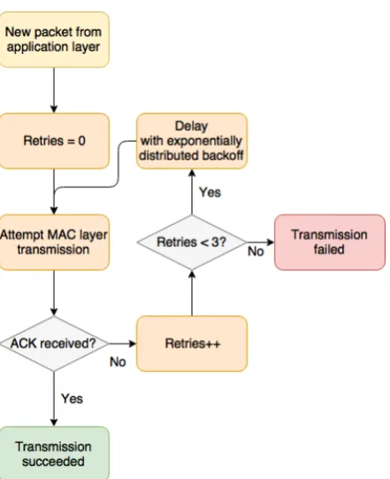
The transport layer model may ensure reliability of the network. The transport layer uses acknowledgment and retransmission with exponentially distributed back-off time. The transport layer retransmits the packet from the application layer to the network layer and the MAC state machine is reset. This happens when no acknowl-edgment has been received and the number of retransmissions has not exceeded the predefined limit. The transport layer waits before the next attempt. A flowchart of the transport layer process is presented in Figure 2.2. The intention of retrans-mission is to increase reliability of the link in unfortunate case of collision.

2.2.3 Network layer model

(21)

[image:21.595.204.425.80.351.2]

bea-2.2. MODEL AND ASSUMPTIONS 15

Figure 2.2: Flowchart of the transport layer with up to 3 retransmissions and expo-nential backoff.

cons use an out-of-band error-, delay- and collission-free channel as in agreement with the scope.

2.2.4 Data link layer model

(22)

chooses a random channel for any channel access. The base station is assumed to be listening on all frequencies and makes no distinction between channels.

2.2.5 Physical layer model

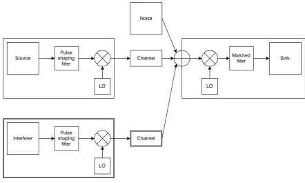
The physical layer gets its data delegated from the MAC layer. The physical layer is responsible for translation of bits in actual signals. This includes pulse shaping, modulation, demodulation, amplification, etc. The traditional approach is a collision model, which does not allow more than a single transmission in the channel. This model is, however, of very limited use for UNB. Due to capture effect there is a probability that one of the two or more frequency overlapping transmissions is re-ceived without error, instead of both packets being dropped. Because of frequency uncertainty there is even likely that two signals on the same channel do not overlap and are received correctly. The additive white Gaussian noise (AWGN) model is introduced to cope with partially overlapping channels and the capture effect.

(23)

[image:23.595.89.532.83.348.2]

Figure 2.3: Block diagram of physical layer model

function of frequency separation (δω) as seen in the equation below.

β(δω) =

n

(pt(−τ)∗pt(τ))·cos(δωτ)

o

∗pr(−τ)∗pr(τ)

τ=0

2Tnpt(τ)∗pt(τ)

o2

τ=0

(2.3)

The rejection coefficient can be calculated for a given pulse shaping filter with im-pulse response pt(τ), matched filter with impulse responsepr(τ)and symbol

dura-tion (T). A derivation for the AWGN contributions can be found in Appendix A. Noise

in the system is modeled as a AWGN with a power level ofN0. The noise power that

remains after the matched filter is the noise coefficient. The effect of this is denoted withγ and is calculated as

γ(N0, Px) =

N0

n

pr(−τ)∗pr(τ)

o

τ=0·

n

pt(−τ)∗pt(τ)

o

τ=0

2T Px

n

pt(τ)∗pt(τ)

o2

τ=0

. (2.4)

In this equation the noise contribution to the SINR can be found, as a function of transmit power (Px), pulse shaping filter impulse response (pt(τ)), matched filter

impulse response (pr(τ)), symbol duration (T) and noise level (N0). As the rejection

(24)

has been applied intentionally by the transceiver and an unknown factor is caused by frequency uncertainty. In the model used here SINR is built up from the three different sources of Figure 2.3, i.e. the intended signal, the interfering signals and the background noise. The signal, interference and noise will result in a varying SINR and therefore a varying bit error rate (BER). The time varying BER is a function of the rejection coefficient, the individual interferers and the noise, as given in Equation 2.5.

BER(t) = 1 2erfc v u u t

2·(

K(t)

X

k=1

β(δω,k) +γ)

−1 !

(2.5)

The BER depends on the number of simultaneous interferers (K) with each a

differ-ent frequency offsetδω,k and the noise coefficient (γ). The probability for a bit error

of bitndepends on the BER at the time of sampling (tn). The SINR can thus be

con-verted in a BER and this is equivalent to the probability of a bit error for a single bit. The probability that a wrong decision is taken at the sampling time corresponds to the BER value at the sampling instant. Lnumber of contiguous bits form a packet, in

which each bit can be erroneous. The PER is equal to the probability that a certain packet has one or more bit errors and is calculated as follows.

P(packet error) = 1−

L−1

Y

n=0

(1−P(bit error of bit n)) (2.6) The PER may be improved by including forward error correction (FEC), the correc-tion will come at the cost of addicorrec-tional bits but may help to recover packets with a few bit errors. Figure 2.4 shows the PER as a function of signal to interference ratio (SIR) and the number of bits that have been under the influence of an interfering signal. If two packets are transmitted at the same time, an SIR of approximately 7 dB is required to have 10% capture probability. The interfering packet will then probably be lost. If 20 bits of an interfering signal arrive at equal strength as the intended packet, both packets have 80% probability of being lost. It can be noted from the graph that a high SIR value gives low probability for packet error. Increasing the time an interferer will also increase the probability of packet errors.

(25)

Figure 2.4: PER performance as function of overlapping bits (L’ out of 160 bits) and SIR without noise.

frequency resulting in the following situation. Because of the frequency uncertainty, two or more signals intended to be transmitted at the same center frequency may end up being frequency multiplexed, in which case the base station may be able to receive all of them. In such a situation the packet delivery ratio (PDR) is much higher than expected based on the single channel assumption. Frequency uncer-tainty should therefore be modeled to retrieve valid FOMs for UNB communication systems. Frequency uncertainty of a crystal is specified by the supplier as a value in ppm. The ppm value corresponds to the maximum expected frequency difference from the nominal frequency. After multiplication by the PLL a 10 ppm oscillator at 868 MHz, may vary between 867.99132 and 868.00868 MHz. To model this, the frequency deviation is randomly picked from a Gaussian distribution [6], withµ= 0 and 3σ = Frequency uncertainty defined in ppm. This ensures 99.7% of the sam-ples δf taken from the distribution are within the specified uncertainty range of the

oscillator. The actual frequency the node is calculated as follows,

fnode =fintended·(1 +δf ∗10−6) (2.7)

Time uncertainty Like frequency uncertainty, time uncertainty comes from the un-certainty of an oscillator. This oscillator is used to keep track of time. A difference in oscillation frequency makes the local time run slower or faster than that of the base station or that of another node. This may cause problems when a rendezvous appointment has been made, but the clocks drift apart. Like frequency uncertainty, time uncertainty is specified in ppm. In case of a 100 ppm crystal oscillator, after 1 day the clocks of unsynchronized nodes in the system may have drifted off ±8.64

(26)

be-cause of time uncertainty is to add guard times between the time slots. Having too long guard times leave the channel unused and causes performance to go down. In UNB systems the time uncertainty will not cause bad performance. Because of the long transmission time for a packet in UNB, the guard time is just a fraction of the total slot time. Even when synchronizing every 100 seconds, having a 100-ppm crystal and 50 time slots, a guard time of 0.01 seconds suffices. This is only 0.5% of the total time. When applying slotted time systems in UNB a small guard time can be used to prevent collision because of time uncertainty. It is therefore not required to model time uncertainty as the expected effect is negligible.

Frequency drift Because the packet transmissions in UNB may take such a long time it may very well be that the frequency of transmission drifts off while transmit-ting. For frequency drift two causes can play a role. The first is Doppler effect due to acceleration, as described in [12]. The second is environmental changes that influence oscillator frequency. Frequency drift due to Doppler effect is very small for a system with a static base station. Acceleration above 10G are not expected, while this results in a frequency drift of only 2.9 Hz/s. The maximum expected frequency drift over a packet duration of 1.6 seconds is then only 4.6 Hz. Compared to the 100 Hz signal bandwidth this effect is negligible. The environmental changes are not ex-pected to have a very high influence. Temperature, pressure, humidity or stress are not expected to change very rapidly, therefore the short term drift of frequency can be neglected. On a longer term the frequency can change. When generating only a few packets per day the frequency of access will be uncorrelated. In this model the frequency drift is neglected, this means that the frequency of any node will not change in the course of simulation.

(27)

Path loss One of the major motivations for this research is the expectation that CSMA performs better than Aloha in a UNB communication system. One of the major drawbacks of CSMA in UNB is the hidden node problem. This is because sensing the channel before transmissions will only increase performance when the business of the channel can be detected reliably. When nodes are too far away to sense each others ongoing transmission a collision occurs. In this research the path loss is modeled as

LP =

Pr

Pt

=Kd0 d

γ

(2.8)

, as explained in [15] section 2.5. In this equation K is a constant representing the

path loss at reference distanced0,γ is the path loss exponent anddis the distance.

In general this model estimates the average effect of distance with exponent γ on

the power received by an antenna. In this modelγdepends on the environment and K on the frequency of operation. Typical values of γ range between 2 and 4. For

this research a value of 3 has been chosen.

In simulation the path loss is determined from the random positioning of the nodes. In this research the nodes are assumed to be uniformly distributed over the area within range of the base station. The sensitivity, transmit power and the path loss exponent are required to determine the range of the base station. A value of -142 dBm is taken as receiver sensitivity of the base station. This value corresponds to the sensitivity of the base station in a Sigfox network [4]. The range that can be achieved with a system operating in the 868-MHz band with a transmit power of 10 dBm is roughly 10 km. The average number of nodes per square meter can be calculated as

Average number of nodes per m2 = M

πd2 m

(2.9)

With M the number of nodes in the network and dm the maximum distance to the

base station in meters. The nodes are placed in simulation using a triangular dis-tribution for the range and a uniform disdis-tribution for the angle. This way the nodes will have a higher probability of being placed far away from the base station. This observation results in a relatively high probability of having hidden nodes, since the distance between nodes is large.

(28)

the PER is higher. In this research the effect of fading is not investigated. However, as described above it will be interesting to investigate the performance of UNB in a channel if average non-fade duration is shorter than the packet length.

2.3 Figures of merit

After a list of MAC layer protocols is created and suitable protocols are selected, it will be time to get some quantitative results from the protocols. The goal is to find the best fit for different operating conditions by comparing the FOMs. The FOMs give important insight in the performance of the MAC protocols. Due to previously given limitations of the model the FOMs may not be achievable in a real scenario.

2.3.1 Packet delivery ratio

PDR is a FOM that gives insight in the reliability of the network. There will always be a possibility that generated packets are lost in the delivery process. This may be due to signal propagation loss, collision, fading dips, congestion in the channel, or any other reason. Packet delivery ratio and its counterpart packet loss probability, or packet drop ratio, are common metrics for capturing WSNs performance. The ratio is calculated as follows [16]

PDR =

P

received packets

P

generated packets (2.10)

In a simulation the PDR achieves its steady state result after some time. PDR will be a value between 0 and 1. A value of 1 means every packet has been delivered successfully. Applications will require a high enough reliability of the link to limit communication errors. This is achieved by having a certain PDR. In this research an arbitrary value of 90% has been chosen. To improve packet delivery ratio there are several options, one of which is to do retransmission after failure. Where this helps to increase packet delivery ratio in noise limited transmission or fading dips, in a congested channel retransmissions will make it worse. The MAC protocol is responsible to prevent congestion. MAC protocols which do prevent congestion effectively are expected to have a higher PDR in high load situations.

2.3.2 Throughput

(29)

2.3. FIGURES OF MERIT 23

represent throughput as the succesful part of the network load, and network load as the ratio of channel usage when packets are perfectly scheduled. The definition is

S = PDR·G= PDR·M·λ·L·T (2.11)

, where G is the network load, M the number of nodes, L packet length and T

symbol duration. This is in accordance with the definition proposed in [10].

The throughput versus network load graph is often seen in MAC protocol re-search such as Aloha or CSMA as given in [7]. The definitions of network load and throughput have been chosen to coincide with the definitions shown in this paper. The resulting performance from simulations in this thesis can thus be directly com-pared to these results. Throughput is always less than the network load. A perfect MAC would increase throughput along with network load until both have value 1. Throughput should not increase beyond this point. However, due to the capture ef-fect and frequency multiplexing the throughput can go up even further. The through-put can be interpreted as the average number of successful transmitted packets on the channel within the observation time. The maximum throughput depends on the ability to frequency multiplex and the ability to reject interference at the base station and to capture the incoming packets.

2.3.3 Network fairness

To measure whether the resources, i.e. the available spectrum, is divided equally be-tween the nodes in the network a measure of fairness is considered. Their are sev-eral different definitions to sense the fairness in a wireless network. Jain et al. [17] propose the so called Jain fairness. This metric is supposed to be independent of the population size (number of nodes). The Jain fairness is both a bounded and a continuous measure of fairness. In wireless networking Jain fairness is calculated on average throughput or average delay per node. Since reduction of delay is not the main design criterion for WSN the throughput has been chosen. Other interest-ing fairness metrics would be the fairness of energy consumption per node. This will make it possible to calculate the battery lifetime expectancy of a node with more certainty. Moreover, a high energy consumption fairness will reduce outage proba-bility in an energy harvesting scenario. We will be considering only Jain fairness on average throughput per node [18]. Jain fairness can be calculated using Equation 2.12,

FJ =

S2 MPM

i=1Si2

(2.12)

, where Si is the throughput for node i, M is the number of nodes and S is the

(30)

usage of the available spectrum and is more applicable for the design of the network. When designing node architecture it may be important to find the fairness in energy consumption. Jain fairness is bounded between 0 and 1. A value of 1 resembles a fair network, where every node has the same probability of delivering its packets to the base station. The distance to the base station is one of the parameters that have large influence on the fairness, because nodes nearby the base station are able to have its packets received with much more power than nodes at the edge of the base station range.

2.3.4 Energy consumption

Energy consumption is, as clarified earlier, one of the major challenges in WSNs. Furthermore, especially the MAC protocol has large impact on the lifetime expec-tancy of a node. An estimation of energy consumption of nodes in a WSN can be found in [19]. Unfortunately the power consumption of the nonexistent hardware is unknown, so most of the parameters described here cannot be filled in. To circum-vent this, a good measure is to capture the average time that the wireless transceiver is on per packet. Energy consumption can roughly be divided into transmission and reception energy, as given in the following equations

Etx=TstartPstart+

n RRcode

(PtxElec+Pamp) (2.13)

Ercvd =TstartPstart+

n RRcode

PrxElec+nEdecBit (2.14)

The energy required for transmission requires a start up of the oscillator and ampli-fier, this is resembled with the time required for startup (Tstart) and the power

con-sumption during startup (Pstart). After the startup has been completed the packet can

be transmitted. The energy budget required for this is the packet transmission time ( n

RRcode) and the power used during transmission (PtxElec). In receive mode the power

for startup and receiving (PrxElec) is equal to that of transmission mode. However,

the receiving part as additional power consumption in the energy required to decode the packet (EdecBit). The startup phase can be neglected because the packet

(31)

2.4. SIMULATION SETUP 25

to complete. It can therefore be concluded that energy consumption is determined mainly by the transmissions of the node. Given consumption during transmission is the main source of energy consumption in a node and the fact that energy is the time integral of power, the total time a node spends in transmission is linearly related to the energy consumption. Keeping track of the time spent in transmission state is therefore a valid FOM to measure energy efficiency. The energy efficiency is then defined as

= Useful energy spent All energy spent =

PDR·T ·L

average time transmitting per packet (2.15)

Retransmissions will cost energy, which would halve the energy efficiency. Prevent-ing retransmissions by doPrevent-ing CCA and reducPrevent-ing collisions is essential for energy efficient MAC protocol operation. A value of 1 would mean the least possible energy is consumed for transmission. Lower values would mean more energy is consumed to transmit a packet or energy is wasted on lost packets.

2.3.5 End-to-end delay

Some applications, such as alarms or control systems, require predictable and low delay to function appropriately [21]. While in this project the delay is not of impor-tance the delay introduced at the MAC layer is not a significant design criterion. In communication systems the delay of a packet is at least the packet transmis-sion time, which is quite high for UNB. Retransmistransmis-sion strategy, beacon interval, contention mechanism and other MAC protocol techniques have an impact on the average time until successful packet delivery. The definition of end-to-end delay is shown in below and has been taken from [16].

D=

PNpackets

i=1 (tsuccess,i−tcreation,i)

Npackets

(2.16)

The average delay (D) is calculated from the number of received packets (Npackets)

and the delay of those packets (tsuccess,i −tcreation,i). The definition only considers

successful packets because it is the most convenient to know how long a packet will take before it is delivered. The lifetime of an unsuccessful packet is not considered and is not important.

2.4 Simulation setup

(32)

based on OMNeT++ that comes close to the required features. However, it requires serious adjustments to be made before it could be used for this research. This means a new framework for simulations in OMNeT++ has to be created. It requires that all subsystems are implemented as in the model presented in Section 2.2. The network in OMNeT++ exists of a number of nodes, which each have an application, MAC protocol implementation and PHY layer implementation to generate packets and transmit the packets at the right time and frequency. The nodes are connected using a channel module, which is responsible for keeping track of all ongoing trans-missions, the calculation of packet errors and the delivery of packets to the base station.

2.4.1 Nodes

A node consists of an application, MAC protocol and PHY layer. The applications keeps generating packets at a specific offered load as a Poisson process. The offered load at which the packets are generated is the network load G divided by

the number of nodes M. If the MAC protocol is still busy with the transmission

of a previous packet the current packet is dropped, this is called the zero buffer assumption. By increasing the number of nodes the probability of having an initially dropped packet becomes very low. It can be so low that the infinite node assumption becomes approximately valid. In simulations the network load is incremented until no further load is required. The load is increased by increasing the offered load per node (λ). This means the number of nodes is fixed for all simulations in that series.

This also means that at high offered loads per node and with a high delay the initial rejection of packets may increase. When that happens the infinite node assumption is not valid anymore. In the simulation framework the nodes are created at startup. This means the positions and the frequency uncertainty do not change during a simulation. This may cause bad accuracy when the number of nodes is low. This effect can be countered by doing multiple repetitions of the same simulation and average the results if required. CSMA like MAC protocols require the possibility to sense the channel before transmission. This is also called CCA. This is done with the same physical layer as for transmission. The received power is integrated over one bit duration to find the RSSI. When the collected energy is higher than a certain value the channel is considered busy and transmission is postponed.

2.4.2 Simulation framework verification

(33)

[image:33.595.98.528.85.285.2]

2.4. SIMULATION SETUP 27

Figure 2.5: Comparison of theoretic and simulated throughput for pure Aloha, slot-ted Aloha and non persistent CSMA.

basic MAC protocols the throughput can analytically be predicted. Pure Aloha, Slot-ted Aloha and non persistent CSMA are a couple of protocols that have well known throughput:

Spure Aloha=Ge−2G

Sslotted Aloha=Ge−G

Snon persistent CSMA =

G G+ 1

(2.17)

(34)

[image:34.595.106.469.101.321.2]

Figure 2.6: Comparison of simulated throughput for pure Aloha, slotted Aloha and non-persistent CSMA under the influence of path loss and retransmis-sions.

Throughput seems to be asymptotic if network load increases The throughput has an asymptotic behavior. In these regions the PDR drops at the same pace as the network load rises. This can be explained as a combined result of the uniform distribution of nodes over the area and no power control. The capture effect causes that only the nearest nodes take part in the delivery process, i.e. the nearest nodes will have the strongest signal. The packets delivered come from a relatively small part of the nodes that are positioned near the base station, the range at which nodes are able to deliver their packets successfully becomes shorter and shorter with increasing network load.

(35)

2.5. SIMULATIONS 29

Performance of Aloha with path loss is generally higher than without path loss Aloha is a just transmit kind of protocol. In the case of zero path loss, both packets are received with equal power, a collision will result in the loss of both packets. When path loss is included the packets arrive with a difference in received power. One of the transmitted packets will have a good chance of being delivered successfully. This results in a higher overall throughput, compared to when no packet has the probability that it arrives free of error.

CSMA performance with path loss is worse than without path loss Sensing the medium has two possible outcomes, it can be either idle or busy and the sensing mechanism can mistake idle for busy and the other way around. Because of the model used here only the average power is measured for sensing the medium. This means the outcome of CCA cannot be busy when it is actually idle. This situation corresponds to the exposed node situation. However, it is possible to measure an idle channel while it is actually free. This happens when the interfering node is further away than the range of CCA. CSMA performance is decreased by those hidden nodes. If all nodes would be hidden CSMA becomes equal to pure Aloha.

Due to retransmissions throughput decreases at high network load Because packets that do not arrive are treated as new arrived packets the effect of retrans-mission can be approximated as an increase of effective network load. At low load the channel may not be completely busy, so there is a chance that a retransmitted packet is delivered correctly after the retry. However, in a busy channel a retrans-mitted packet causes imminent collision and will lead to lower throughput. It can be concluded that retransmission in this form is effective, because without any form of frequency multiplexing the maximum operable network load is 1.

2.5 Simulations

(36)

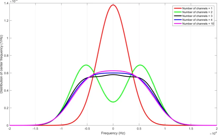
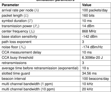
channel protocols is the number of channels times the throughput of a single chan-nel. However, because of inter channel interference this will either not be efficient in terms of spectrum usage or the total throughput will be lower. Comparing single channel with multi channel protocols in a fair manner is a challenging task, because multi channel protocols cannot be converted into single channel protocols. However, the other way around is true. In simulation this is done by placing channels next to each other in frequency domain. Because of frequency uncertainty, the channels may have significant overlap, but this is accounted for by changing the channel sep-aration accordingly. In the limit of number of channels going to infinity, the multi channel protocol becomes a CR-FDMA protocol. It may be possible that reducing the number of channels, thus increasing the separation, will have a positive effect on the performance of a certain protocol. However, if the protocol performs best at high number of channels, the CR-FDMA variant will be the more optimal solution for that MAC protocol. The distribution of center frequencies in a multi channel MAC proto-col, subject to frequency uncertainty, is shown in Figure 2.7. Because of the infinite character of the Gaussian distribution it will not be possible to prevent any node from sending outside the intended bandwidth. The separation of the channels is tuned such that for a given number of channels the spillover of the overall frequency distribution is 5%. As the number of channels is increased the distribution of the center frequency becomes more and more uniform. It is expected that this uniform distribution, which corresponds to the CR-FDMA protocols, is the optimal solution for frequency multiplexing in UNB. The multi channel counterparts of Pure Aloha or Slotted Aloha are the ones described and proposed by [23], namely frequency unslotted time unslotted Aloha (FU-TU-Aloha) and frequency unslotted time slotted Aloha (FU-TS-Aloha). frequency slotted time unslotted Aloha (FS-TU-Aloha) and frequency slotted time slotted Aloha (FS-TS-Aloha) are frequency slotted versions, so they have a non-uniform distribution for center frequency like shown in Figure 2.7. These protocols are expected to have worse performance than the unslotted versions. Each simulation run consists of a number of nodes with random fixed position and frequency deviation. The number of nodes is chosen such that a rep-resentative simulation is achieved. Because of the no buffering assumption, there will be initial rejections of packets when the MAC protocol is busy with the previous packet. The parameters of the MAC protocols and network parameters are the same in all simulations. The chosen values are defined in Table 2.1.

(37)

2.5. SIMULATIONS 31

(a)A 1-ppm crystal reference in 868-MHz band distributed within 10 kHz bandwidth.

[image:37.595.138.498.417.641.2]

(b)A 10-ppm crystal reference in 868-MHz band distributed within 20 kHz bandwidth.

(38)

Simulation parameters

Parameter Value

arrival rate per node (λ) 100 packets/day

packet length (L) 160 bits

symbol duration (T) 10 ms

transmission power (Px) 14 dBm

center frequency (f0) 868 MHz

base station sensitivity -142 dBm

path loss exponent 3

noise floor (N0) -174 dBm/Hz

CCA measurement delay 10 ms

CCA busy threshold 6.3096e-20 J

retransmissions 3

average time before retransmission (exponential) 10 s

slotted time guard 34.56 ms

beacon interval 100 beacons/day

[image:38.595.98.472.265.575.2]

multi channel bandwidth (1 ppm) 10 kHz multi channel bandwidth (10 ppm) 20 kHz

(39)

2.5. SIMULATIONS 33

that they do not violate regulations of the 868-MHz band. The bandwidth is chosen such that the simulations will be feasible. The guard time between slots is chosen such that worst case clock skew (with a 10-ppm crystal) will not result in collisions as in [24].

2.5.1 Single channel simulation

Single channel simulation will be done on all single channel MAC protocols that come through the selection procedure described in Section 2.1. It is assumed that all single channel MAC protocols, transformed into a multi channel protocol will have similar improvements. This is because all MAC protocols of a category use the same technique for medium access. If there is a reason to suspect a MAC protocol being different from others, a new category can be introduced. The single channel MAC protocols will be judged based on a smaller set of FOMs, namely PDR, throughput (S) and energy efficiency (). One of the basic constraints of having a working

system is to have a good PDR. The minimum PDR to have a good communication system for this work is set to 90%, and the corresponding offered network load G0

is given as in

G0 =G(PDR = 0.9) (2.18)

The PDR is expected to be monotonically decreasing from1to0with increasing net-work load. Therefore, the selection of 90% will always result in a single intersection. Within each category the throughput and energy efficiency are taken at the network load (G0) where PDR is 90%, then normalized to the maximum of that category and

summed to retrieve the final score, as in

score = S(G0) maxSc

+ (G0) maxc

(2.19)

This score is relative to each category. It basically scores the relative improvements of throughput and energy efficiency compared to other protocols in the category. The MAC protocol within each category with the highest score is selected for multi channel simulation. It is assumed that the unselected MAC protocols, which perform poorly in single channel simulations, would not outperform the other MAC protocols of that category in multi channel simulations. Therefore, by following this approach, the multi channel simulations, that would produce uninteresting results, are avoided.

2.5.2 Multi channel simulation

(40)

(41)

Chapter 3

Results

In this chapter the results of the tests and simulations are presented. This is per-formed along the method described in Chapter 2. The chapter starts with a selection of the protocols that are included into the project. Then the single channel protocols will be compared and selected in Section 3.2. In Section 3.3 the multi channel sim-ulation is performed and the resulting FOMs for the protocols are presented.

3.1 MAC protocol selection

In Table 3.1 the results from protocol selection are shown. Only some of the best fitted protocols are shown, since the list would otherwise be too long. The protocols which do not satisfy the requirements are given in Appendix B.

Each of the protocols belong to a certain category and may have multi channel capabilities. The selection and categorization can be seen in Table 3.2.

3.2 Single channel simulation

For single channel simulation the MAC protocols from Table 3.2 are implemented and put to the test. Only the single channel protocols from the table are used for single channel comparison. The other MAC protocols are simulated in multi channel simulation and compared with multi channel variants of the single channel protocols. SIFT is a protocol that is expected to outperform other types of persistent CSMA protocols, because of its supposed optimized contention strategy. The resulting scores, as defined in Equation 2.19, are given in Table 3.3.

The MAC protocols with the highest score in the single channel simulations are selected to be simulated in a multi channel simulation. These MAC protocols are Slotted Aloha, non persistent CSMA and ISMA. However, because multi channel transformation will not give a practical solution for idle sense multiple access (ISMA)

(42)

Protocol 1.1 2.1 2.2 3.1 3.2 4.1 4.2 4.3 4.4

[Liu:2014] [25] X X X X X X X

Alert [26] X X X X X X X X

BP-MAC [27] X X X X X X X X

BPS-MAC [28] X X X X X X X X

CSMA/CA [29] X X X X X X X X

CSMA/p* [30] X X X X X X X X

CSMA-TDMA Hybrid [31] X X X X X X X X

DSA++ [32] X X X X X X X

EY-NPMA [33] X X X X X X X X X

FS-TS-Aloha [23] X X X X X X X X X

FS-TU-Aloha [23] X X X X X X X X X

FU-TS-Aloha [23] X X X X X X X X X

FU-TU-Aloha [23] X X X X X X X X X

ISMA [34] X X X X X X X X X

MASCARA [34] X X X X X X X

nanoMAC [35] X X X X X X X X

non persistent CSMA [36] X X X X X X X X X

persistent CSMA [36] X X X X X X X X X

Pure Aloha [36] X X X X X X X X X

R-ISMA [34] X X X X X X X X

RMAC [37] X X X X X X X X

SIFT [38] X X X X X X X X X

Slotted Aloha [36] X X X X X X X X X

TDMA [36] X X X X X X X X

[image:42.595.82.491.183.646.2]

Others... See Appendix B

(43)

3.3. MULTI CHANNEL SIMULATION 37

Protocol Category Single channel

BPMAC Listen before talk X

BPSMAC Listen before talk X

EY-NPMA Listen before talk X

FS-TS-Aloha Contention FS-TU-Aloha Contention FU-TS-Aloha Contention FU-TU-Aloha Contention

ISMA Collision avoidance X

non persistent CSMA Listen before talk X

Pure Aloha Contention X

SIFT Listen before talk X

[image:43.595.144.484.85.318.2]

Slotted Aloha Contention X

Table 3.2: Selected protocols and categorization.

that protocol will not be considered. The multi channel protocols from Table 3.2 will be and they are the multi channel counterparts of the Aloha type protocols.

3.3 Multi channel simulation

All FOMs are captured in the simulation. The simulation is done in the case of both 1 ppm or 10 ppm with a variable number of channels and for 10 kHz and 20 kHz bandwidth.

Simulations are performed up to a network load of 400 Erlang. In case of a perfect MAC protocol the bandwidth of 20 kHz gives room for approximately 200 channels, each with a maximum network load of 1 Erlang. Since the ideal MAC behavior is not likely to be achieved, a throughput of at most 100 Erlang can be expected.

In figures 3.1 to 3.6 the results of multi channel simulation for the selected pro-tocols are visible as a function of frequency uncertainty and number of channels. The number of channels that perform best in terms of the score at a PDR of 0.9 are compared between each other. These results are given in Table 3.4.

(44)

Category FU (ppm) Protocol G0 S score Position

Contention

0 Slotted Aloha 0.90 0.80 0.39 1.70 1 Pure Aloha 0.24 0.21 0.56 1.26 2

Listen before talk

0

np CSMA 0.30 0.26 0.64 1.91 1

SIFT 0.33 0.29 0.57 1.89 2

BPMAC 0.29 0.25 0.63 1.85 3 BPSMAC 0.29 0.25 0.62 1.85 4 EY-NPMA 0.32 0.28 0.56 1.84 5

1

np CSMA 2.19 1.97 0.63 2.00 1 BPMAC 2.11 1.89 0.61 1.94 2 BPSMAC 2.10 1.88 0.61 1.93 3

SIFT 2.18 1.95 0.54 1.86 4

EY-NPMA 2.18 1.95 0.54 1.85 5

10

np CSMA 23.86 21.35 0.68 2.00 1 BPMAC 22.71 20.35 0.66 1.92 2 BPSMAC 22.64 20.29 0.65 1.91 3 SIFT 23.36 20.88 0.59 1.85 4 EY-NPMA 23.64 21.14 0.58 1.85 5

Collision avoidance

0 ISMA 0.46 0.41 0.51 2.00 1

1 ISMA 2.76 2.48 0.52 2.00 1

[image:44.595.64.510.88.557.2]

10 ISMA 24.65 22.04 0.61 2.00 2

Table 3.3: Per category results of single channel simulation.

Number of channels 6 12 18 24

1 ppm

FS-TU-Aloha 1.45 1.88 1.99 1.95 FS-TS-Aloha 1.56 1.95 1.97 1.97 non persistent CSMA 1.54 1.95 1.95 1.98 Number of channels 2 3 4 10

10 ppm

FS-TU-Aloha 1.82 1.98 1.93 1.92 FS-TS-Aloha 1.98 1.92 1.92 1.86 non persistent CSMA 1.88 2.00 1.98 1.94

[image:44.595.124.447.578.721.2]

(45)

[image:45.595.134.495.119.344.2]

Figure 3.1: FS-TU-Aloha (Pure aloha) multi channel simulation results with 1 ppm frequency uncertainty.

[image:45.595.132.495.467.689.2]

(46)

[image:46.595.104.466.120.342.2]

Figure 3.3: FS-TS-Aloha (Slotted Aloha) multi channel simulation results with 1 ppm frequency uncertainty.

[image:46.595.105.466.466.690.2]

(47)

[image:47.595.136.494.120.344.2]

Figure 3.5: Non persistent CSMA multi channel simulation results with 1 ppm fre-quency uncertainty.

[image:47.595.132.497.466.689.2]

(48)

[image:48.595.92.472.130.352.2]

Figure 3.7: Comparison of PDR for multi channel MAC protocols for 1 ppm.

[image:48.595.99.474.474.700.2]

(49)

[image:49.595.124.502.124.347.2]

Figure 3.9: Comparison of energy efficiency for multi channel MAC protocols for 1 ppm.

[image:49.595.129.503.476.701.2]

(50)

[image:50.595.95.473.130.353.2]

Figure 3.11:Comparison of fairness for multi channel MAC protocols for 1 ppm.

[image:50.595.91.475.470.698.2]

(51)

[image:51.595.122.501.124.348.2]

Figure 3.13: Comparison of throughput for multi channel MAC protocols for 10 ppm.

[image:51.595.123.503.460.683.2]

(52)

[image:52.595.102.474.129.353.2]

Figure 3.15: Comparison of delay for multi channel MAC protocols for 10 ppm.

[image:52.595.93.476.474.698.2]

(53)

Chapter 4

Discussion

In this chapter the results of simulations are analyzed and discussed. This chapter goes step wise through the methodology applied to discuss the results and to give comments as to why the results are what they are.

4.1 MAC protocol selection

The MAC protocol selection starts with a very large list of which only very few are suitable for further analysis. Many of the dropped protocols have implemented a combination of different layers that built upon a certain basic MAC protocol. While combining MAC protocols with other layers may be beneficial, the protocols that do this cannot be compared fairly to MAC protocols that do not do this. Therefore, only the most basic protocols remain for simulation in this research.

4.2 Single channel simulation

The results of single channel simulation present the effect of frequency uncertainty on MAC protocol performance. Each category has been studied and a comparison has been made between the MAC protocols within that category. Some observations can be made about the results. These are treated per category. Observations of the reference simulations for verification have already been given in Section 2.4.2. The results have been processed into the form of a table to calculate the relative scores. The results of single channel simulation which are referred to in this discussion are in Table 3.3.

(54)

4.2.1 Contention

In the contention category there are pure Aloha and slotted Aloha. For each of the simulated frequency uncertainties the slotted Aloha protocol outperforms pure Aloha protocol. This can be explained by the time slotted operation of slotted Aloha. In a time slotted system no partial collisions will appear, such that the channel is bet-ter used. With increasing frequency uncertainty more packets can be successfully transmitted at the same time. While this increases throughput of the contention pro-tocols, the bandwidth used for the single channel expands. The effect of frequency uncertainty is roughly the same for both protocols. In other words, since the packets have equal delivery probability the required amount of energy does not change.

4.2.2 Listen before talk

The LBT MAC protocols are SIFT, non-persistent CSMA, BPMAC, BPSMAC and EY-NPMA. SIFT protocol uses a persistent type of CSMA with an optimal distribution for contention resolution. BPMAC, BPSMAC and EY-NPMA use preambles to notify other nodes of an imminent packet as contention resolution. The protocols that use contention resolution are outperformed by the non-persistent CSMA, which doesn’t have contention resolution. This can be explained with the used model. Contention resolution does only work when two or more nodes are attempting to access the channel at the same time, given they are not hidden nodes. Furthermore, the con-tention resolution requires time to give every node a turn. In the Poisson process the probability of two packets being generated at the same time is very low and the rate at which packet are generated does not allow time for the channel to elimi-nate a congested state of the network. In the Poisson process the probability of time synchronous transmissions does not outweigh the little overhead introduced for con-tention resolution. The effect of frequency uncertainty is similar as in the concon-tention protocols.

4.2.3 Collision avoidance

(55)

collision avoidance which tries to minimize collisions from hidden nodes, of which there are quite a lot.

4.3 Multi channel simulation

In multi channel simulation the best MAC protocols per category of single channel simulation are compared with each other. The distribution of the center frequency used by a node depends on the number of channels (channel chosen with equal probability and equal spacing) and the frequency uncertainty. The multi channel simulation gives a comparison of performance including the effect of frequency mul-tiplexing.

4.3.1 FS-TU-Aloha

In the case of FS-TU-Aloha, the multi channel counterpart of pure Aloha, the number of channels does make a clear difference for 1 ppm case, as seen in Figure 3.1. For the 10-ppm crystal (Figure 3.2) the FOMs are almost similar. This is due to the shape of the distributions for center frequencies, as can be seen in Figure 2.7. As the 1 ppm case has more resemblance with the uniform distribution of CR-FDMA these results can be trusted when it comes to the number of channels. The scores of FS-TU-Aloha for 18 and 24 channels do not change much just as their frequency distributions.

4.3.2 FS-TS-Aloha

Just as in FS-TU-Aloha, in FS-TS-Aloha the results of figures 3.3 and 3.4 show good behavior for high number of channels in the case of 1 ppm and a low number of channels in the case of 10 ppm. In the 10-ppm case the low number of channel performs slightly better than the high number of channels. This is a remarkable feature. However, since it is not like this for 1 ppm it cannot be concluded that less channels will be better.

4.3.3 Non-persistent CSMA

(56)

any of the number of channels. However, when looking at the scores from Table 3.4 2 channels is performing slightly worse than the other number of channels.

4.3.4 Comparison

The comparison of the FOMs for the best performing MAC protocols in 10 and 20 kHz bandwidth can be found in figures 3.7 to 3.16.

Packet delivery ratio What one can obtain clearly from Figure 3.7 is that FS-TS-Aloha outperforms the other protocols based on PDR. Especially when looking at 90% value, the FS-TS-Aloha performs better than the other protocols. With a much higher network load the CSMA protocol takes over. The same goes approximately for 10 ppm frequency uncertainty, as seen in Figure 3.12.

Throughput For throughput the same arguments apply as in PDR, since the two are highly related. This can be seen in figures 3.8 and 3.13. There is some strange behavior happening at FS-TU-Aloha throughput at very high network load. The throughput goes up again, this can be explained as a side effect of the simulations that may be introduced because of the capture effect and the low number of nodes that contribute to the performance. The region where this effect happens is not of interest to anyone who uses the system as it as less than 30 % packet delivery ratio.

Energy efficiency The energy efficiency can be compared from figures 3.9 and 3.14. The energy efficiency goes down quite fast. The network is therefore best run at a low network load. For both 1 and 10 ppm cases the energy efficiency is best at non-persistent CSMA.

Delay All protocols have comparable average delay, which can be seen in figures 3.10 and 3.15. The least delay occurs at FS-TS-Aloha, because it requires less retransmissions. Since the number of attempts of non-persistent CSMA is limited, the delay is also bounded. This ensures good behavior in terms of the FOMs, but additional delay may be traded off at the gain of PDR. In the region of low network load FS-TS-Aloha has slightly higher delay because of the packets that have to wait before a new time slot starts.

(57)

(58)

(59)

Chapter 5

Conclusions and recommendations

Suitable MAC protocols for a UNB communication system have been collected and compared based on their performance in a single channel and multi channel envi-ronment. Path loss and frequency uncertainty are physical effects that have been modeled. Retransmissions have been used to upgrade the reliability of the protocol. The results for the situations have been explained in Chapter 4. In this chapter the conclusions are drawn from the results of simulation and in Section 5.2 recommen-dations are made for follow-up research.

5.1 Conclusions

Based on the simulations presented in the results chapter it can be concluded that path loss is one of the physical effects that has a large influence on MAC proto-col performance. It causes hidden nodes and allows for capture effect. Where the capture effect poses an improvement of throughput, the same cannot be said for hidden nodes. Hidden nodes make that CSMA protocols perform even worse than slotted Aloha or FS-TS-Aloha, while in theory its performance should be much bet-ter. A quantitative conclusion cannot be drawn on the effect of hidden nodes for CSMA protocols, because only one situation of hidden nodes is researched. Colli-sion avoidance or reservation protocols will not be suitable for UNB communication systems with rare, short packets.

The effect of frequency uncertainty is large on single channel UNB networks, because of the small signal bandwidth compared to the large frequency uncertainty. This enables the ability to have frequency multiplexing on a single channel, such that no errors are caused. However, it does require an intelligent receiver to find and demodulate all the signals. This will be possible in a star topology, where the base station is equipped with unlimited resources.

In a multi channel network the frequency division access technique that shows