Extremum statistics: a framework for data analysis

University of Warwick institutional repository: http://go.warwick.ac.uk/wrap

This paper is made available online in accordance with

publisher policies. Please scroll down to view the document

itself. Please refer to the repository record for this item and our

policy information available from the repository home page for

further information.

To see the final version of this paper please visit the publisher’s website.

Access to the published version may require a subscription.

Author(s): S. C. Chapman1, G. Rowlands1, and N. W. Watkins2

Article Title: Extremum statistics: a framework for data analysis

Year of publication: 2002

Link to published version:

http://www.nonlin-processes-geophys.net/9/issue5_6.html

Publisher statement: The original authors and citation details must be

identified. Chapman, S.C. et al. (2002). Extremum statistics: a

Nonlinear Processes in Geophysics (2002) 9: 409–418

Nonlinear Processes

in Geophysics

c

European Geosciences Union 2002

Extremum statistics: a framework for data analysis

S. C. Chapman1, G. Rowlands1, and N. W. Watkins2

1_{Physics Department, University of Warwick, Coventry CV4 7AL, UK}

2_{British Antarctic Survey, High Cross, Madingley Rd., Cambridge CB3 0ET, UK}

Received: 24 October 2001 – Revised: 21 January 2002 – Accepted: 8 February 2002

Abstract. Recent work has suggested that in highly cor-related systems, such as sandpiles, turbulent fluids, ignited trees in forest fires and magnetization in a ferromagnet close to a critical point, the probability distribution of a global quantity (i.e. total energy dissipation, magnetization and so forth) that has been normalized to the first two moments fol-lows a specific non-Gaussian curve. This curve folfol-lows a form suggested by extremum statistics, which is specified by a single parametera(a=1 corresponds to the Fisher-Tippett Type I (“Gumbel”) distribution).

Here we present a framework for testing for extremal statistics in a global observable. In any given system, we wish to obtaina, in order to distinguish between the dif-ferent Fisher-Tippett asymptotes, and to compare with the above work. The normalizations of the extremal curves are obtained as a function ofa. We find that for realistic ranges of data, the various extremal distributions, when normalized to the first two moments, are difficult to distinguish. In ad-dition, the convergence to the limiting extremal distributions for finite data sets is both slow and varies with the asymptote. However, when the third moment is expressed as a function ofa, this is found to be a more sensitive method.

1 Introduction

The study of systems exhibiting non-Gaussian statistics is of considerable current interest (see, e.g. Sornette, 2000, and references therein). These statistics are often observed to arise in finite sized, multi-body systems, exhibiting correla-tion over a broad range of scales, leading to emergent phe-nomenology, such as self-similarity and in some cases frac-tional dimension (Bohr et al., 1998). The apparent ubiquitous nature of this behavior has led to interest in self-organized criticality (Bak, 1997; Jensen, 1998) as a paradigm; other highly correlated systems include those exhibiting fully

de-Correspondence to: S. C. Chapman ([email protected])

veloped turbulence. In solar terrestrial physics in particu-lar, problems of interest include MHD turbulence in the so-lar wind and in the Earth’s magnetotail. Irreguso-lar or bursty transport and energy release in the latter has recently led to complex system approaches such as SOC (see the review by Chapman and Watkins, 2001). These complex systems are often characterized by a lack of scale, and in particular, by the exponents of the power law probability distributions (PDF) of patches of activity in the system. Examples of these patches of activity include energy dissipated by avalanches in sandpiles, vortices in turbulent fluids, ignited trees in forest fires and magnetization in a ferromagnet close to the critical point. In the Earth’s magnetotail, patches of activity in the aurora, as seen by POLAR UVI have been used as a proxy for the energy released in bursty magnetotail transport, in or-der to infer its scaling properties (Lui et al., 2000; Uritsky et al., 2001). The challenge is to distinguish the system from an uncorrelated Gaussian process, by demonstrating self-similarity and to determine the power law exponents. To do this directly is nontrivial, requiring measurements of the in-dividual patches or activity events over many decades. Here we consider what may be a more readily accessible measure: the statistics of a global average quantity, such as the total energy dissipation, magnetization and so forth.

These studies reveal statistics of a global quantity (i.e. E) that follow curves that are of the form of one of the limit-ing extremal distribution (Gumbel, 1958; Fisher and Tippett, 1928):

P (E)=K(ey−ey)a y=b(E−s), (1)

where K, b ands are obtained by normalizing to the first two moments (M0 = 1,M1 = 0,M2 = 1), and the single parameteraappears to be close to the valueπ/2.

For an infinitely large ensemble, there are two limiting dis-tributions that we consider here. The Fisher-Tippett type I (or “Gumbel”) extremal distribution is of the form (1), but witha =1 and arises from selecting the largest events from ensembles with distributions that fall off exponentially or faster. Since we wish to construct a framework that could encompass all highly correlated systems, we also treat the case where the distribution of “patches” is a power law. An example is the Potts model (Cardy, 1996) for magnetization, where connected bonds form clusters, the size of which is power law distributed at the critical point. In this case, the relevant extremal distribution is Fisher-Tippett type II (or “Frechet”).

Here we provide a framework for comparing data with Fisher-Tippett type I and II extremal curves. This essentially requires obtaining the normalizations of these curves in terms of the moments of the data and ultimately as functions of the single parametera.

We find that the curves of form (1), which are obtained by normalizing to the first two moments, are difficult to distin-guish ifais in the range(1,2)or from Frechet curves given a realistic range of data. Furthermore, we demonstrate that slow convergence with respect to the size of the data set, to the limitinga =1 extremal distribution has the consequence that, for a large but finite ensemble, the extremal distribu-tion of an uncorrelated Gaussian process is indistinguishable from thea =π/2 curve. To overcome these limitations we suggest two much more sensitive methods for determining whether or not the curve is of the form (1), and, if so, the corresponding value ofa. These methods are based on the third moment, and the peak of the distribution, both of which we obtain here as a function ofa.

2 Extremum statistics: general results

To facilitate the work here we first develop some results from extremum statistics (for further background reading, see Sor-nette (2000); Gumbel (1958); Bouchaud and Potters (2000)). If the maximumQ∗drawn from an ensemble ofMpatches of activityQwith distributionN (Q)isQ∗=max{Q1, ..QM}, then the probability distribution (PDF) forQ∗is given by Pm(Q∗)=MN (Q∗)(1−N>(Q∗))M−1, (2) whereMis the number of patches in the ensemble and

N>(Q∗)= Z ∞

Q∗

N (Q)dQ. (3)

We now obtainPmfor largeM, Q. For general PDFN (Q) we can write (for appropriate choice of the functiong(Q∗)): (1−N>)M =e−Mg(Q

∗

) ₍₄₎

and for smallN>(Q∗)we have

g(Q∗)= −ln(1−N>(Q∗))∼N>+

N_>2

2 . (5)

We now consider a characteristic value ofQ∗, namelyQ˜∗, such that by definition

Mg(Q˜∗)=q, (6)

so that

q =Mg(Q˜∗)≈MN>(Q˜∗)+M

N_>2(Q˜∗)

2 + · · ·. (7)

We now expandg(Q∗)about_Q˜∗_{to obtain}

g(Q∗)=g(Q˜∗)+g0(Q˜∗)1Q∗+g 00_(Q˜∗₎

2 (1Q

∗

)2+ · · ·(8)

and from (5) we have

g0(Q∗)= −N (Q∗)−N (Q∗)N>+ · · · (9)

g00(Q∗)= −N0(Q∗)−N0(Q∗)N>+N2(Q∗)+ · · ·, (10) where g0, g00 denote differentiation with respect to Q∗, 1Q∗ = Q∗− ˜Q∗, and we have usedN_>0 =dN>/dQ∗ = −N. Inverting expansion (7) gives

MN>(Q˜∗)=q h

1− q 2M + · · ·

i

≈M1−e−Mq

. (11)

We obtain from (5) and its derivatives with respect toQ∗: g(Q˜∗)= q

M

1− q 2M

+1

2 q

M 2

+ · · ·

= q M +0

q M

3

, (12)

which to relevant order is consistent with (6), and

g0(Q˜∗)= −N (Q˜∗)h1+ q M + · · ·

i

. (13)

Forq finite asM → ∞this givesg0(Q˜∗)= −N (Q˜∗)and MN>(Q˜∗)=q.

We can now consider the extremal statistics of specific PDFN (Q), and more importantly show thatPm(Q∗)can be written in the universal form (1).

2.1 Gaussian and ExponentialN (Q)

IfN (Q)falls off sufficiently fast inQ, i.e. is Gaussian or ex-ponential, it is sufficient to consider lowest order only in (5) givingg(Q∗)∼N>(Gumbel, 1958; Bouchaud and Mezard, 1997) andq = MN>(Q˜∗). Expanding (3) inQ∗nearQ˜∗ gives to this order:

MN>(Q∗)=M Z ∞

˜ Q∗

N (Q)dQ−MN (Q˜∗)1Q∗

=q "

1−MN ( ˜ Q∗)

q 1Q

∗_{+ · · ·} #

≈qe−M

N (_Q˜∗₎

q 1Q

∗

S. C. Chapman et al.: Extremum statistics: a framework for data analysis 411

ExpandingN (Q)aboutQ∗yields

N (Q∗)=N (Q˜∗) "

1+N 0_(Q˜∗₎

N (Q˜∗₎1Q ∗_{+ · · ·}

#

≈N (Q˜∗)e

N0(_Q˜∗₎

N (_Q˜∗₎1Q ∗

. (15)

As to this order(1−N>)M−1≈e−MN> we then have from (2)

Pm(Q∗)=MN (Q∗)(1−N>(Q∗))M−1

≈MN (Q∗)e−MN> _∼(eu−eu₎a_{, (16)}

with

a= −N 0_(Q˜∗_)N

>(Q˜∗)

N2_(Q˜∗₎ (17)

and

u=ln MN>( ˜ Q∗₎

a !

− N ( ˜ Q∗) N>(Q˜∗)

1Q∗. (18)

Since throughout we are consideringQ˜∗to be large (M→ ∞, qfinite), we have the effective value ofaas that given by (17) in the limitQ˜∗→ ∞. ForN (Q)exponential the above givesa=1. In the particular case of the exponential, all the summations, which in the above we have truncated, can be resummed exactly and givea ≡ 1, recovering the result of Bouchaud and Mezard (1997).

ForN (Q) Gaussian we cannot obtain a exactly in this way, but as we shall see it is instructive to make an estimate. Given N (Q) = N0exp(−λQ2) and expanding Eqs. (14), (15) and (16) to next order we obtain

Pm= ¯PmeR(u)

R= −ln 2_(q) 4λQ˜∗2 + ¯u

1+2 ln(q) 4λQ˜∗2

− u¯ 2 4λQ˜∗2−e

¯

u_{, (19)}

where we have usedu= −2λQ˜∗1Q∗andu¯=u+ln(q). To lowest order in1Q∗/Q˜∗(i.e.Q˜∗→ ∞) we have a universal PDF witha = 1, but to next order, i.e., neglecting only the term inu¯2in (19), we have a universal distribution of form (1,16) with

a≡

1+2 ln(q) 4λQ˜∗2

6=1. (20)

2.2 Power lawN (Q)

The PDF of patches N (Q)may, however, be a power law and in this case it will fall off sufficiently slowly withQso that we need to go to next order, as in (7). If we consider a normalizable source PDF

N (Q)= N0

(1+Q2₎k, (21)

then for largeQ(Q 1) we haveN (Q) ∼ N0/Q2k and then using (3) and (7)

˜

Q∗N (Q˜∗)

=(2k−1)N>(Q˜∗)=(2k−1)

q M(1−

q

2M), (22)

which with the above general expressions forg(Q˜∗)and its derivatives substituted into (8) gives an expression forg(Q∗) g(Q∗)=

q M

1−(2k−1)1Q

∗ ˜

Q∗ +k(2k−1)(

1Q∗ ˜ Q∗ )

2_{· · ·}

.(23)

We also require an expression forN (Q∗), again expanding aboutQ˜∗and obtaining the derivatives ofN (Q˜∗)from those ofg(Q˜∗)and via (11) gives

N (Q∗)=N (Q˜∗)

1−2k1Q

∗ ˜

Q∗ +k(2k+1)(

1Q∗ ˜ Q∗ )

2

,(24)

which can be rearranged as

N (Q∗)=N (Q˜∗)e h

−2k1Q_˜∗

Q∗ +k( 1Q∗

˜

Q∗ ) 2i

. (25)

After some algebra (23) can be rearranged to give

Mg(Q∗)=qe h

−(2k−1)1Q_˜∗

Q∗ + 2k−1

2 ( 1Q∗

˜

Q∗ ) 2i

. (26)

These two expressions combine to finally give

Pm(Q)≡Pm(Q∗)∼(eu−e¯

¯

u

)a (27)

with

¯

u= −ln(a)−ln(q)−(2k−1)1Q

∗ ˜ Q∗ (1−

1Q∗

2Q˜∗) (28) and

a= 2k

2k−1. (29)

To lowest order, neglecting the (1Q∗/Q˜∗)2 term (28) re-duces to (18).

Hence, a power law PDF has maximal statisticsPm(Q) which, when evaluated to next order, can be written in the form of a universal curve (i.e. of form (1,16)) with a cor-rection that is non-negligible at the asymptotes. This can be seen (Jenkinson, 1955; Bouchaud and Potters, 2000) to be consistent with the well-known result due to Frechet, where (following the notation of Bouchaud and Potters, 2000) if we have PDF

N (x)∼ 1

|x |1+µ, (30)

then

N>∼ 1

xµ (31)

Pm(x∗)=

µ (x∗₎1+µe

− 1

which we can write in the form

Pm(x∗)=µe

µ+1 µ ln(

µ+1

µ )_(eu−eu₎a ₍₃₂₎

u= −µln(x∗)−ln _µ+1

µ

, (33)

which is of universal form (1,16) inu. Noting that hereµ= 2k−1 anda=(µ+1)/µand that to second order

1Q∗ ˜ Q∗ (1−

1Q∗ 2Q˜∗)=ln

1+1Q ∗ ˜ Q∗

, (34)

we simply identify 1+1Q∗/Q˜∗withx˜∗to obtain (28). To next order in1Q∗/Q˜∗ the analogue of (28) still yields the right-hand side of (34).

2.3 Convergence to the limiting distributions

The above results should be contrasted with the derivation of Fisher and Tippett (Fisher and Tippett, 1928). Central to Fisher and Tippett (1928) and later derivations is that a single ensemble ofN Mpatches has the same statistics as theN en-sembles (ofMpatches), of which it is comprised. The fixed point of the resulting functional equation (Bhavsar and Bar-row, 1985) for arbitrarily largeNandMisa=1 for the ex-ponential and Gaussian PDF, and the Frechet result for power law PDF. Here we consider a finite sized system so that al-though the number of realizable ensembles of the system can be taken to be arbitrarily large, the number of patchesMper ensemble is always large but finite. More importantly, the rate of convergence withMdepends on the PDFN (Q). For an exponential or power law PDF we are able to resum the above expansion exactly to obtaina and convergence then just depends on termsO(1/M)and above. This procedure is not possible forN (Q)Gaussian, instead we consider the characteristicQ∗, that isQ˜∗ which forM to be arbitrarily large,Q∗should be large as well. Rearranging (7) to lowest order forN (Q)=N0exp(−λQ2)yields

√ λQ˜∗∼

√ ln(M), implying significantly slower convergence. This is further discussed in Sornette (2000).

The extremal distributions are thus essentially a family of curves that are approximately of universal form (1,16) and are asymmetric with a handedness that just depends on the sign ofQ; we have assumedQto be positive, whereas one could chooseQto be negative, in which caseN (Q)→N (| Q|). This would correspond to, say, power absorbed, rather than emitted, from a system. The single parameterathat dis-tinguishes the extremal PDF then just depends on the PDF of the individual events. ForN (Q)exponential we then recover exactly the well-known result (Gumbel, 1958; Bouchaud and Mezard, 1997)a=1. For a power law PDFais determined bykvia (29). We have also demonstrated that for a Gaussian PDF with finite but largeMandN, thata 6=1 and we will explore the significance of this in Sect. 3.1.

3 Normalization to the first two moments

To compare these curves with data we needP (Q)¯ ≡Pm(Q∗) in normalized form. This has moments

Mn = Z ∞

−∞

ynP (y)dy,¯ (35)

which we will obtain as a function ofa and then insist that M0=1,M1=0 andM2=1.

SettingM1 = 0 (andM0 = 1,M2 = 1) in our analysis of extremal distributions does not require any assumptions about the form of the PDF except that the moments exist. It will allow us to write the analytically obtained extremal distributions as functions of single parametera.

3.1 Extremal distributions arising from Gaussian and expo-nentialN (Q)

For Gaussian and exponential PDF we have

¯

P (y)=K(eu−eu)a (36)

u=b(y−s). (37)

This has moments which converge for alln. From Appendix A we have that thent hmoment:

Mn = 1 b

Z ∞ −∞

¯

P (y)dη[ln(a)+bs−η]

n

bn

=Ke−aln(a) d

n

dan0(a), (38)

whereη=ln(a)−u.

To normalize we insist thatM0=1,M1=0 andM2=1. The necessary integrals can be expressed in terms of deriva-tives of the Gamma function0(a)(Gradshteyn and Ryzhik, 1980) and we obtain in Appendix A:

b2=90(a)

K= b

0(a)e

aln(a) ₍₃₉₎

s= −(9(a)−ln(a))

b ,

where

9(a)= 1 0(a)

d0(a) da

90(a)=d9 da.

The ambiguity in the sign ofb(and hences) corresponds to the two solutions forP (Q)¯ for positive and negativeQ.

S. C. Chapman et al.: Extremum statistics: a framework for data analysis 413

−10 −8 −6 −4 −2 0 2 4

10−5

10−4

10−3 10−2

10−1

100

y

P

−10 −8 −6 −4 −2 0 2 4 10−5

10−4

10−3

10−2

10−1

100

Fig. 1. Curves of the form (1) fora = 1, π/2,2. Overlaid (*)

are the numerically calculated extremal statistics of an uncorrelated Gaussian process (see text), and inset for comparison are Frechet curves plotted on the same scale (see Fig. 2).

dynamic range of about 4 decades, something which is not readily achievable.

In Fig. 1 we have also over plotted (*) the extremal PDF of ensembles of uncorrelated numbers that are Gaussian dis-tributed, calculated numerically. We randomly selectM un-correlated variablesQj, j =1, Mand to specify the hand-edness of the extremum distribution, theQj are defined neg-ative andN (|Q|)is normally distributed. This would phys-ically correspond to a system where the global quantityQ¯ is negative, i.e. power consumption in a turbulent fluid, as op-posed to power generation. To construct the global PDF we generateT ensembles, that is selectT samples of the largest negative numberQ∗_i = min{Q1..QM}i, i = 1, T. For the data shown in the figureM =105andT =106, this gives √

λQ˜∗ ∼ √

ln(M) '3 so that for the Gaussian we are far from thea=1 limit (Fisher and Tippett, 1928). The numer-ically calculated PDF lies close toa =π/2. Such a value of aon these curves thus does not give direct evidence of a cor-related process; in addition, it is necessary to establish that the data considered do not arise as the result of an extremal process.

Generally, plotting data in this way is an insensitive method for determiningaand thus distinguishing the statis-tics of the underlying physical process. The question of in-terest is whether we can determine the form of the curve, and the value ofa from data with a reasonable dynamic range; we address this question in Sect. 4.

3.2 Frechet distributions arising from power lawN (Q)

For power law PDF (21) we use the Frechet distribution which we first write as:

P (Q∗)=K(eu−eu)a (40)

u=α+βln(1+Q ∗ ˜

Q∗), (41)

which reduces to the form of (37) for1Q∗/Q˜∗ 1. From (28), (21) and (33) we identify

β = −µ= −(2k−1). (42)

The procedure of normalizing to the moments is only valid provided that they exist. For the power law PDF (21) we have (see also Bury, 1999):

Mn = Z ∞

0

QnH (Q)dQ (1+Q2₎k ,

which converges forQ→0 and forQ→ ∞

Mn ∼

Z ∞_Qn_{H (Q)dQ} Q2k , which ifH (Q)→H0asQ→ ∞

Mn →

Z ∞ _dQ Q2k−n '

1

Q2k−n−1 |Q→∞, which converges if 2k > n+1.

We now evaluate the moments. Again, we insist thatM0= 1,M1=0 andM2=1 and in Appendix B obtain:

α= −βln 

 a1β

0(1+1/β) 



K= ±βaa

0(1+ 2 β)−0

2₍₁₊ 1 β)

1₂

(43)

˜

Q∗₌ 0(1+

1

β) h

0(1+2

β)−02(1+

1

β) i1₂

,

whereβ = −(2k−1). The normalization constants are thus also expressible as functions ofa=2k/(2k−1).

For convergence, these curves exist for power law of index ∞ > 2k > 3 i.e. 1 < a < 3/2. This is significant since processes exhibiting intermittency as a consequence of long-range correlations typically havek lower than this (Jensen, 1998), and we will consider alternative methods in Sect. 5.

−10 −8 −6 −4 −2 0 2 4

10−5

10−4

10−3

10−2

10−1

100

Q*

P(Q*)

k=2

k=5

k=100

Fig. 2. Frechet PDF normalized to the first two moments for PDF

N (Q)=1/(1+Q2)k,k=2,5,100.

4 Sensitive indicators ofa; the mean and the third mo-ment

The question of interest is whether we can determinea with sufficient accuracy from data with a reasonable dynamic range. We consider two possibilities here. First, a uniformly sampled process will have the most statistically significant values on the extremal curve near the peak, and in particu-lar, from the figures we see that the Frechet distributions for smallkwill be most easily distinguished in this way. For the Frechet PDF the peak is atu=0, i.e., it has coordinates

¯ Pm=

K

ea y¯= ˜Q h

e−αβ −1i (44)

on the normalized curve withK,Q, α, β˜ known as functions ofa from Appendix B. The coordinates of the peak of the PDF from the data plotted withM0=1, M1=0 andM2= 1 can thus be graphically inverted to give an estimate ofa.

For PDF that represent a power law with largek, either ex-ponential or Gaussian, we consider the normalized extremal PDF; then the coordinates of the maximum of P (y)¯ is at u=0,y=s, i.e.:

¯ Pm=

K ea =

√

90_(a)e−a(1−ln(a))

0(a) (45)

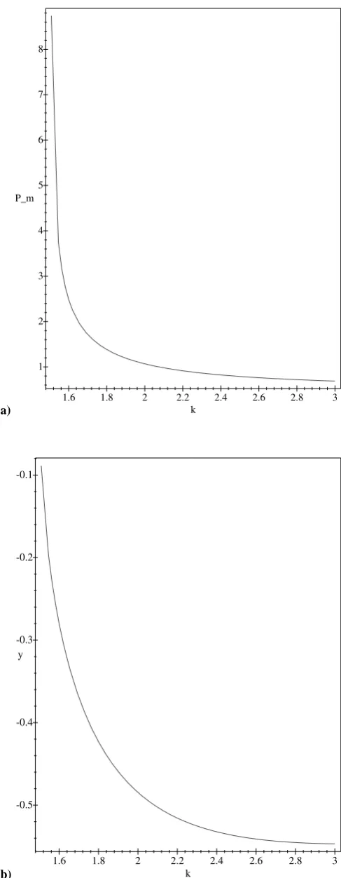
withK, s from (A14). These can again be graphically in-verted to obtaina; Fig. 3 showsP¯ andy¯ versusk for the Frechet PDF.

A more sensitive indicator may be the third moment ofP¯ of the curve (1,16), which, after some algebra (Appendix A), can be written as

M3= − 9 00_(a)

(90_(a))3₂

(46)

(a) 1.6 1.8 2 2.2k 2.4 2.6 2.8 3

P_m 8

7

6

5

4

3

2

1

(b) k

3 2.8 2.6 2.4 2.2 2 1.8 1.6 y -0.1

-0.2

-0.3

-0.4

-0.5

Fig. 3. The peak (a) and its location (b) as a function of k for

S. C. Chapman et al.: Extremum statistics: a framework for data analysis 415

for a Gaussian or exponential PDF, i.e. with (37) and

M3= h

0(1+ 3

β)−30(1+

2

β)0(1+

1

β)+20

3₍₁₊1

β) i

h 0(1+ 2

β)−02(1+

1

β) i3₂

(47)

for a power law PDF (Appendix B), i.e. with (41); the lat-ter then converging for k > 2. Again, these refer to one of the two possible solutions for P (Q)¯ ; the other solution corresponding toy → −y (Q∗ → −Q∗) in Eqs. (37) and (reffrechu) which in turn givesM3→ −M3.

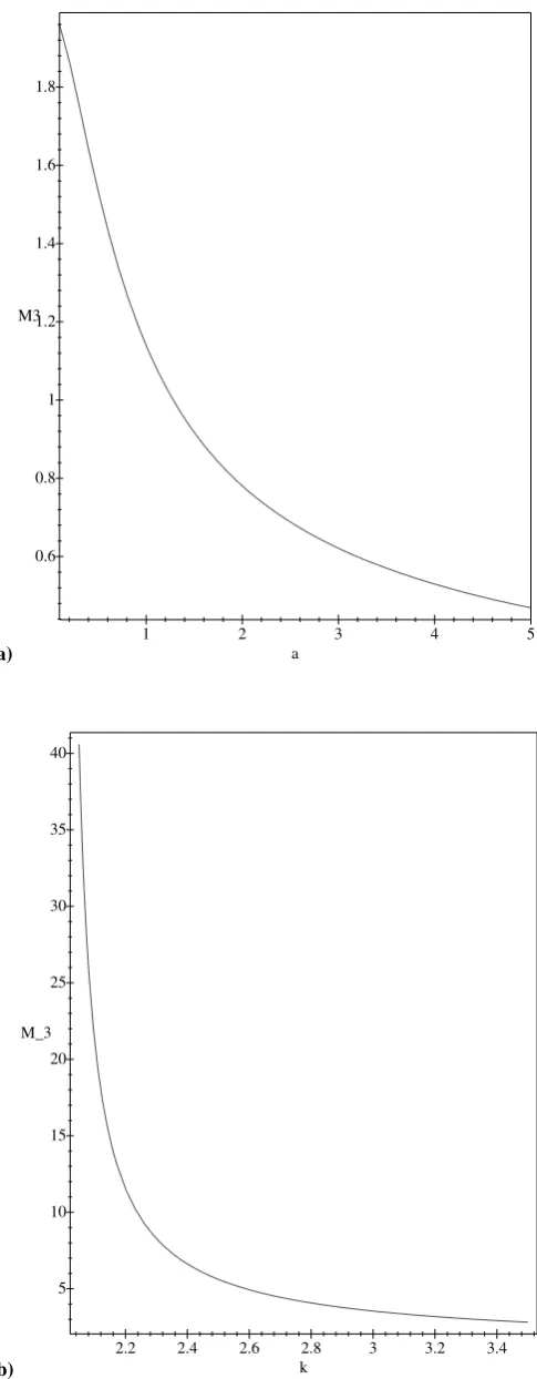
The third moment is plotted versusa andk, respectively, in Fig. 4 for the Gumbel and Frechet curves. Inspection of Fig. 4 shows that over most of the range,M3is more sensitive thanP¯. For Frechet curves, M3 only has convergence for relatively largek (k > 2, a < 4/3); for smallerk,P¯ can distinguish the Frechet distributions (k > 3/2, a <3/2 for convergence).

5 A method for smallk

ForN (Q)power law, we can only use the properties of the normalized Frechet PDF above fork >3/2. Ifkis smaller than this the second moment will not exist. We can, however, obtain a useful result fork > 1 by using the first moment only, i.e. by insistingM0 = 1, M1 = 0. We need another condition and can arbitrarily insistP (u=0)=1 (insisting that all the maxima of the Frechet PDF have the same height) which gives the condition

Ke−a =1. (48)

From B6 and B5

KQ˜∗

βg1/β_aa =1, (49)

which, withg1/β=0(1+1/β)from Appendix B, givesQ˜∗ in terms ofa andβ (ork). Similarly, we use (B5);g=aeα to obtainαin terms ofaandβ.

This then gives

Pm(Q∗)=K

eu−eua,

u=α+βln(1+1Q ∗ ˜ Q∗ ),

α=βln

0(1+1 β)

−ln(a),

˜

Q∗=βea(ln(a)−1), K=ea.

6 Conclusions

Recent work has suggested that the probability distribution of some global quantity, such as total power needed to drive ro-tors at a constant velocity in a turbulent fluid, or total magne-tization in a ferromagnet slightly off the critical point, when

(a) 1 2 a 3 4 5

M3 1.8

1.6

1.4

1.2

1

0.8

0.6

(b) k

3.4 3.2 3 2.8 2.6 2.4 2.2 M_3

40

35

30

25

20

15

10

5

Fig. 4. The third moment as a function ofafor (a) curves of form

normalized to the first two moments, follows a non-Gaussian, universal curve. This curve is of the same form as that found from the extremal statistics of a process that falls off expo-nentially or faster at large values (i.e. Fisher-Tippett type I or “Gumbel”); whereas for an extremal process, the param-eter specifying the curvea =1, for the correlated processes a >1.

In this paper, a framework has been developed to com-pare data with Fisher-Tippett type I (“Gumbel”) and type II (“Frechet”) asymptotes by obtaining the curves, and their normalizations, as a function of a single parametera. We find:

1. The Fisher-Tippett type I and type II curves and their corresponding values ofaare most easily distinguished by considering either the third moment, or the position of the peak, as functions ofa, the functional forms for which are given here.

For realistic ranges of data, simply comparing curves normalized to the first two moments, for example, in Bramwell et al. (1998, 2000), is insufficient to ade-quately distinguish either curves of the form of type I (“Gumbel”) but witha values in the range [1,2], or most type II (“Frechet”) curves.

2. Convergence to the limiting form of the extremal curve a=1 (Gumbel’s asymptote Fisher and Tippett (1928)) is sufficiently slow for an uncorrelated Gaussian such that for a large but realistic size of data set one obtains a ≈π/2. Data that falls on this curve is thus not suffi-cient to unambiguously distinguish a global observable of a system that has correlations (Bramwell et al., 1998, 2000), from that of an uncorrelated, extremal process.

Comparison with data is then facilitated in the following way. First, the data distribution is normalized toM0(to ob-tain the PDFN (Q)). Second, the data is plotted on semilog axes under the following normalization:N (Q)×M2versus (Q−M1)/M2. Any Gaussian PDF on such a plot will fall on a single inverted parabola; similarly, any Gumbel (Fisher-Tippett I) process will fall on a single curve. Finally,M3is calculated for the data; we then can compare the data with an extremal process by inverting M3(a) obtained here for a Fisher-Tippett type I or II distribution. Overlaying these curves (augmented by other quantitative comparisons) then essentially constitutes a fitting procedure; but more impor-tantly, in addition, the value ofais related to the underlying distribution, as we have discussed.

This and related techniques will have relevance, in partic-ular, for regions where transport is dominated by turbulence, in the solar wind and magnetosphere in circumstances where multi-point and long time interval in situ measurements are difficult to obtain.

Acknowledgements. The authors would like to thank G. King,

M. P. Freeman, D. Sornette and J. D. Barrow for illuminating discussions. SCC was supported by PPARC.

Appendix A Moments of the Gumbel distribution and the normalizationb,Kandsas a function ofa

We consider a family of curves of the form

P (y)=Ke−au−ae−u (A1)

withu=b(y−s)whereK, b, s, are constants to be derived as functions ofa. We write

η=lna−b(y−s)=lna−u, (A2)

thenae−u = eη anddη = −bdy, and the nth moment is given by

Mn = Z ∞

−∞

ynP (y)dy= 1 b

Z ∞ −∞

P (y)dη[ln(a)+bs−η]

n

bn . (A3)

Then, using A2, we writeP (y)(A1) as

P (y)=K e−a(ln(a)−η)−eη= ¯Keaη−eη, (A4) whereK¯ =Ke−aln(a).

Now to within a constant we can writeMnas:

˜ Mn =

Z ∞ −∞

ηnP (y)dη= ¯K Z ∞

−∞

ηneaη−eηdη, (A5)

so that M0 = M0/b˜ . Using the substitution τ = eη A5 becomes

˜ Mn = ¯K

Z ∞

0

(lnτ )nτa−1e−τdτ = ¯K d

n

dan0(a), (A6)

where0(a)is the Gamma function. Thus

˜

M0= ¯K0(a) ˜

M1= ¯K0(a)9(a)= ˜M09(a) ˜

M2= ¯K0(a)[92(a)+9

0

(a)]

= ˜M0(92(a)+90(a)), (A7)

where

9(a)=d0(a) da

1

0(a).

We now insist thatM0=1,M1=0 andM2=1. Thus

M0= ˜ M0

b =

¯ K0(a)

b =1 (A8)

and

M1=0= 1 b2

Z ∞ −∞

P (y)dη[ln(a)+bs−η]

= 1 b2

h

(ln(a)+bs)M˜0− ˜M1 i

, (A9)

so

˜ M1

˜ M0

S. C. Chapman et al.: Extremum statistics: a framework for data analysis 417

from A7. Thus

bs=9(a)−ln(a). (A11)

Also,

M2=1= 1 b3

Z ∞ −∞

P (y)dη[ln(a)+bs−η]2

= 1 b3

h

(ln(a)+bs)2M0˜ −2(lna+bs)M1˜ + ˜M2 i

, (A12)

which, using A7 and A10, rearranges to give

M2=1= ˜ M0

b39

0

(a). (A13)

This finally gives the normalisation of the universal curve

b2=90(a) ¯

K= b

0(a)

that isK= b 0(a)e

aln(a) _(A14)

s=(9(a)−ln(a))

b .

The above results will also yield an expression for the third moment in terms ofa. Following A3 and A5 we have

M3= 1 b4

Z ∞ −∞

P (y)dη[ln(a)+bs−η]3

= 1 b4

h

(ln(a)+bs)3M0˜ −3(lna+bs)2

˜

M1+3(ln(a)+bs)M2˜ − ˜M3i. (A15)

Then A6 gives

˜ M3=

˜

M0h9(a)(92(a)+90(a))+29(a)90(a)+900(a)i(A16)

which, with A7 and A10, rearranges to give

M3= −

900(a)

(90(a))3/2. (A17)

Appendix B Moments of the Frechet distribution and normalization as a function ofa.

The moments of a Frechet distribution are obtained from Bury (1999). Here we wish to consider PDF of the form (19) which has extremum statistics

Pm(Q)=K(eu−e

u

)a, (B1)

where, following (25–32), we write:

u=α+βln(1+Q ˜

Q), (B2)

where here we use the notationsQ≡1Q∗,Q˜ ≡ ˜Q∗, i.e.Q refers to extremal values. From (26),αandβ =(2k−1)are constants. We can then define the moments ofPm(Q):

Mn = Z ∞

− ˜Q

QndQ Pm(Q) (B3)

since from B2u→ ∞asQ→ ∞andu→ −∞asQ→ − ˜Q. Using the substitutionaeu = ζ we obtain after some algebra

Mn = ¯KQ˜n Z ∞

0 ((ζ

g)

1/β₋₁₎n_ζa−1+1/β_e−ζ_{dζ, (B4)}

where the constants

g=aeα and K¯ = K ˜ Q

βgβ1_aa

. (B5)

By taking the expansionu=α+βQ/Q˜it is straightforward to verify that B4 yields the results from Appendix A. We now insist thatM0=1,M1=0 andM2=1. B4 then gives

M0=1= ¯K0(a),¯ where a¯=a+1/β (B6) and

M1=0= ¯KQ˜[0(a¯+1/β)

g1/β −0(a)¯ ], that is

0(a¯+ 1 β)=g

1/β_{0(a)¯ (B7)}

and using B7 we have from B4:

M2=1= ¯KQ˜2[

02(a)0(¯ a¯+2/β)

02_(a¯+1/β) −0(a)¯ ], that is

1= ˜Q2[0(a)0(¯ a¯+2/β)

02_(a¯+1/β) −1] (B8)

using B6.

Now from the main text (27)a = 2k

2k−1 and since β = −(2k−1)

¯

a =a+1/β =1 (B9)

and0(a)¯ =0(1)=1.

B7 then givesg1/β =0(1+1/β). B8 then givesQ˜:

˜

Q= ± 0(

1+ 1 β) h

0(1+2

β)−02(1+

1

β) i1₂

(B10)

then B7 gives K as

K= ±βa

a_0(1+1/β) ˜

Q (B11)

and sinceg=aeα, B6 gives an expression forα:

(aeα)1β ₌ K

˜ Q

that is:

α= −βln 

 a1β

0(1+1/β) 

 (B13)

which completes the normalization of B1,B2 as functions of kora.

Using B7 we have from B4 an expression for the third mo-ment:

M3= ¯KQ˜3

h0(a¯+_β3)03(a)¯ 03_(a¯+1

β) −

30(a¯+2 β)0

2_(a)¯ 02_(a¯+1

β)

+

30(a¯+ 1 β)0(a)¯

0(a¯+ 1 β)

−0(a)¯ i. (B14)

Expansion in 1/β readily shows that to lowest order result A17 is recovered.

Then, using B9, B10 and B11, B13 can be rearranged to giveM3(β), and hence,M3as a function ofkora:

M3= h

0(1+ 3

β)−30(1+

2

β)0(1+

1

β)+20

3₍₁₊1

β) i

h 0(1+ 2

β)−02(1+

1

β) i3₂

. (B15)

References

Aji, V., and Goldenfeld, N.: Fluctuations in finite critical and turbu-lent systems, Phys. Rev. Lett., 84, 1007–1010, 2001.

Bak, P.: How nature works: the science of self-organised criticality, Oxford University Press, Oxford, 1997.

Bhavsar, S. P. and Barrow, J. D.: First ranked galaxies in groups and clusters, Mon. Not. Roy. Astron. Soc., 213, 857–869, 1985. Bohr, T., Jensen, M. H., Paladin, G., and Vulpiani, A.:

Dynami-cal systems approach to turbulence, Cambridge University Press, Cambridge, 1998.

Bouchaud, J. P. and Mezard, M.: Universality classes for extreme value statistics, J. Phys. A, 30, 7997, 1997.

Bouchaud, J. P. and Potters, M.: Theory of financial risks: from sta-tistical physics to risk management, Cambridge University Press,

Cambridge, 2000.

Bramwell, S. T., Holdsworth, P. C. W., and Pinton, J. F.: Univer-sality of rare fluctuations in turbulence and critical phenomena, Nature, 396, 552–554, 1998.

Bramwell, S. T., Christensen, K., Fortin, J. Y., et al.: Universal fluctuations in correlated systems, Phys. Rev. Lett., 84, 3744– 3747, 2000.

Bramwell, S. T. et al.: Reply to comment on “universal fluctuations in correlated systems”, Phys. Rev. Lett., 87, 18 8902, 2001. Bury, K.: Statistical distributions in engineering, Cambridge

Uni-versity Press, Cambridge, 1999.

Cardy, J. E.: Scaling and renormalization in statistical physics, Cambridge University Press, Cambridge, 1996.

Chapman, S. C. and Watkins, N. W.: Avalanching and

self-organised criticality: a paradigm for geomagnetic activity?, Space. Sci. Rev., 95, 293–307, 2001.

Fisher, R. A. and Tippett, L. H. C.: Limiting forms of the frequency distribution of the largest and smallest members of a sample, Proc. Camb. Phil. Soc., 24, 180–190, 1928.

Gradshteyn, I. S. and Ryzhik, I. M.: Table of integrals, series and products, Academic Press, 1980.

Gumbel, E. J.: Statistics of extremes, Columbia university press, New York, 1958.

Jenkinson, A. F.: The frequency distribution of the annual max-imum (or minmax-imum) values of meteorological elements, Q. J. Roy. Meteorological Soc., 81, 158–171, 1955.

Jensen, H. J.: Self-organised criticality: emergent complex be-haviour in physical and biological systems, Cambridge Univer-sity Press, Cambridge, 1998.

Labbe, R., Pinton, J. F., and Fauve, S.: Power fluctuations in turbu-lent swirling flows, J. Phys. II, France, 6, 1099–1110, 1996. Lui, A. T. Y., Chapman, S. C., Liou, K., Newell, P. T., Meng, C. I.,

Brittnacher, M., and Parks, G. K.: Is the dynamic magnetosphere an avalanching system?, Geophys. Res. Lett., 27, 911–915, 2000. Pinton, J. F., Holdsworth, P., and Labbe, R.: Power fluctuations in a closed turbulent shear flow, Phys. Rev. E, 60, R2452–R2455, 1999.

Sornette, D.: Critical phenomena in the natural sciences – chaos,

fractals, selforganization and disorder: concepts and tools,

Springer, Berlin, 2000.

Uritsky, V. M., Klimas, A. J., and Vassiliadis, D.: J. Geophys. Res., submitted, 2001.