Philip A. Trostel
Department of Economics University of Warwick
Coventry CV4 7AL Great Britain Tel: (44) 24 7652 3034 Fax: (44) 24 7652 3032
E-mail: [email protected]
March 2000
Abstract
This study examines a crucial assumption in much of the recent work
on endogenous growth, namely, constant returns to scale in the
production of human capital. A simple model is constructed to show
that the returns to scale in human capital production can be inferred
from the relationship between the wage rate and years of schooling.
A large international micro dataset is used to estimate this
relationship. The empirical evidence is decisive. There are
decreasing returns to scale in human capital production; that is, the
micro-level evidence is not supportive of endogenous growth driven
by human capital accumulation.
JEL Codes: O41, J24, I21
*I am very grateful to Andrew Oswald, Gaelle Pierre, Eric Schansberg,
1There have been over forty such studies published within the
last decade or so. A few examples are Lucas (1988), King and Rebelo (1990), Rebelo (1991), Jones et al. (1993), Mulligan and Sala-i-Martin (1993), and Stokey and Rebelo (1995).
2In a related vein, Saint-Paul (1996) and Acemoglu (1996) derive
increasing (pecuniary) returns in human capital accumulation based on labor market frictions and the assumption of constant (technological) returns to scale in producing human capital.
3Decreasing returns to scale are imposed in the empirical work
by Haley (1976) and Heckman (1976). Constant returns are effectively imposed in Ben-Porath (1970) and Rosen (1976).
In recent literature endogenous long-run growth is explained by
the accumulation of "broadly defined" capital. Typically it is the
inclusion of human capital into the analysis which generates
endogenous growth.1 Growth is created in these models by assuming
that the capital stocks are produced through constant returns to
scale functions of inputs that can be accumulated, i.e., the capital
stocks. These constant returns to scale assumptions induce
endogenous gr owth by creating returns to investments which
perpetually exceed their costs. Thus net investment in the capital
stocks never ceases, which leads to perpetual growth.
An important problem with this class of endogenous growth
models, however, is that there is no empirical evidence to support
the crucial assumption of constant returns to scale in human capital
production.2 The limited microeconomic evidence on human capital
production is not helpful in this regard as it has imposed important
restrictions on the estimates of the returns to scale to the inputs
that can be accumulated.3 And the macroeconomic evidence on human
4The evidence in Romer (1990), Barro (1991), and Tallman and
Wang (1994) is consistent with the notion that human capital accumulation drives long-run growth; while the evidence in Mankiw et al. (1992), Romer (1994), Benhabib and Spiegel (1994), and Jones (1995) is inconsistent with the hypothesis; and the evidence in Barro and Sala-i-Martin (1992, 1995) is inconclusive. These conflicting results may not be surprising, however, given the great difficultly in distinguishing between theories using macro data, especially in this case because of the lack of good data on human capital [on this issue see Benhabib and Jovanovic (1991), Levine and Renelt (1992), Levine and Zervos (1993), and Pack (1994)].
inconclusive.4
Moreover, there is no compelling intuitive reason to believe
that there are constant returns in producing human capital. Although
constant returns in providing educational services (i.e., teaching)
follows from a standard replication argument, this does not imply
constant returns to scale in producing human capital. Human capital
is obviously embodied in individuals (an important fact that is
glossed over in the common two-sector endogenous growth models), and
the most important input in its production is the time individuals
spend learning - an input which is not obviously replicatable.
Hence, the replication argument for constant returns to scale does
not apply to human capital production.
This study attempts to redress this important shortcoming in
the understanding of the forces of long-run economic growth. A
simple model is constructed to show that the returns to scale in
human capital production (from education) can be inferred from the
rate of return to education. In particular, the shape of the
rate-of-return function follows the returns to scale (from the inputs that
can be accumulated) in the human capital production function. If
there are constant (increasing, decreasing) returns to scale in
5Endogenous growth driven by human capital is still possible
with decreasing private returns to human capital if there are sufficiently large external returns. Limited empirical evidence, however, suggests that this is unlikely. Wyckoff's (1984) estimate of the external benefit from educational human capital (for grades K-12, where the marginal external benefits are presumably larger than for higher education) is 9 percent of the private benefit (and is not statistically significant). Moreover, the vast majority of the models of endogenous growth driven by human capital assume constant private returns to scale [some notable exceptions are Lucas (1988), Mulligan and Sala-i-Martin (1993), and Barro and Sala-i-Martin (1995)].
return to education is constant (rising, declining).
Data from the International Social Survey Programme is used to
estimate (private) marginal rates of return to education. This data
on over 30,000 working-age men in 26 different countries decisively
rejects a constant marginal rate of return to education (i.e.,
constant returns to scale in producing human capital). More
precisely, the marginal rate of return is significantly increasing
at low levels education (thus indicating significant increasing
returns), and the marginal rate of return is decreasing significantly
at high levels education (thus indicating significant decreasing
returns).
In other words, the data indicates that the human capital
production function has a cubic shape; that is, this production
function has the shape that is typically taught in introductory
microeconomics courses. The implication of this is that, after about
twelve years of education, there are significant decreasing (private)
returns to the inputs that can be accumulated. Thus the
applicability of endogenous growth models driven by human capital
accumulation is doubtful.5
6Blinder and Weiss (1976) and Rosen (1976) use an alternative,
but essentially equivalent, definition: human capital is produced linearly but is non-linearly related to productivity.
7Depreciation of human capital does not affect any of the
subsequent analysis, hence it is ignored.
Following standard practice, human capital is defined such that
it linearly increases labor productivity and hence the wage rate, w:6
(1) w = rH,
where r is the rental rate on human capital, H. Human capital
accumulation is assumed to be governed by the production function
(2) dHt/dt = Nx"ty(tH*t,
where t is the time instant, x is time invested in human capital, y
is goods (i.e., the services from teachers, physical capital, etc.)
invested in human capital,
N is a productivity parameter (i.e.,
learning ability), and
",
(, and
* are returns elasticities.
7 If aninterior solution is imposed (which is not necessary in this
analysis), then there must be decreasing returns to x and y together
(i.e.,
" +
( < 1). But this does not restrict the returns to the
inputs that can be accumulated (i.e.,
( +
*), which is what matters
for endogenous growth.
Following Haley (1976), the first-order conditions for optimal
production can be used to substitute y out of the production
function. In particular, equation (2) becomes
(3) dHt/dt = Mxt"+(H t(+*,
where M
/
N((r/"p)(, and p is the price of y.capital production are years of school, thus the focus here is on
human capital from education. If each year of full-time schooling
is assumed to take an equal input of time, then x is constant during
schooling and the production function can be further simplified. In
particular, setting this constant to unity, without loss of
generality, makes the human capital production function
(4) dHt/dt = MHFt for 0 < t
#
S,where
F
/
( +
* (the returns elasticity to the inputs that can be
accumulated), and S is cumulative years of schooling.
Differential equation (4) is a Bernoulli equation with constant
coefficients. The solution to this equation at the end of schooling
is
:
H0eMS if F = 1,
=
(5) HS =;
=
<
(H01-F+(1-F)MS)1/(1-F) if F…
1,where H0 is the human capital stock prior to schooling. Substituting
equation (5) into equation (1) and taking the logarithm yields
:
ln(r) + ln(H0) + MS if F = 1,=
(6) ln(w) =
;
=
<
ln(r) + (1-F)-1ln(H01-F+(1-F)MS) if F
…
1.Ideally the
F could be estimated from non-linear equation (6),
but this is not feasible. The data are insufficient to identify H0
and
M. And, more importantly, the data indicates that
F varies
substantially with the level of S. An alternative strategy is to
test the restriction implied by
F = 1. That is, equation (6) shows
that the returns to scale in human capital production can be inferred
8
M
ln(w)2/M
2S = (F-1)M2(H01-F+(1-F)MS)-2. This term is negative
(positive) if F < 1 (> 1).
9See the surveys by Psacharopoulos (1985,1994).
10The following assumptions (plus the assumption that
F = 1) are
also made (usually implicitly) in practically all of the literature on the rate of return to education.
11See, for example, Hungerford and Solon (1987), Kroch and
Sjoblom (1994), Groot and Oosterbeek (1994), Weiss (1995), Heckman et al. (1995), Jaeger and Page (1996), Park (1999), and Chevalier and years of schooling. A linear relationship implies that there are
constant returns to the inputs which can be accumulated. A concave
(convex) empirical relationship between ln(w) and S indicates that
there are decreasing (increasing) returns.8
The effect of S on ln(w) is typically interpreted as the rate
of return to education and has been estimated literally hundreds of
times.9 Thus, the test for non-constant returns to scale is also a
test for a non-constant rate of return to education. In other words,
the simple model above suggests that an observed constant (declining,
rising) marginal rate of return to education indicates constant
(diminishing, increasing) returns in producing human capital through
education.
This result is intuitive and fairly obvious once shown. The
simple model above, however, clearly shows the assumptions that
underlie the conclusion that the returns to scale can be inferred
from the observed relationship between years of schooling and its
marginal rate of return. Some discussion of some of these
assumptions is in order before turning to the evidence.10
Schooling is assumed to have a productive role rather than a
screening role. Although there is some evidence in favor of
Walker (1999).
research on schooling assumes that it is indeed productive (i.e., it
produces human capital). Moreover, the idea of endogenous growth
driven by human capital accumulation can be dismissed immediately if
schooling is not socially productive. Thus this complication is not
addressed here.
The model above solves for the level of human capital at the
completion of formal schooling. Clearly, however, wages will also
depend on human capital acquired through on-the-job training.
Following the empirical work on the rate of return to education,
(potential) work experience polynomials are included as control
variables in the regressions. Typically a second-order experience
polynomial is used, but Murphy and Welsh (1990) argue that a
fourth-order polynomial is more appropriate. A fourth-fourth-order polynomial is
used here, but the results are essentially unchanged when using a
second-order polynomial (and also when including an
experience-schooling interaction term along with either a second- or
fourth-order polynomial).
The first-order conditions for optimal production were used to
substitute goods invested in human capital out of the production
function. The assumption of an optimal mix of inputs may seem
untenable given that most y is publicly provided. But all that is
really required to justify the above simplification is the assumption
that y is proportionally related to H, which seems reasonable.
The model also assumes that each year of schooling requires an
equal input of time (x = 1
œ
S). Casual evidence suggests thatx increases with S there will be a bias in the data toward increasing
returns. On the other hand, however, the data on schooling is
typically grade completed, as opposed to years in school. This will
create a bias toward decreasing returns to the extent slow learners
(ie, those whose grade is less than their years in school) obtain
lower levels of S and fast learners (grade greater than their years)
obtain higher levels of S.
Finally, the model implicitly assumes that education is
uncorrelated with unobservables which independently affect human
capital and wages. But, as stressed by Card (1995), this is
unlikely. Higher-ability individuals are likely to obtain higher
levels of both schooling and wages, other things equal. Thus, Card
contends that unaccounted for differences in ability could make
concave rate-of-return/schooling relationships for individuals appear
linear across individuals. Although not emphasized by Card, the same
can be said for more motivated individuals, for individuals attending
better schools, and for individuals raised in more nurturing homes.
In each case, these unobservables are likely to create a bias in the
data towards increasing returns.
Recent work on the rate of return typically attempts to deal
with this problem by using "natural experiments" to instrument for
education. But, again as stressed by Card (1995), this procedure
will generally yield an unbiased estimate of the average marginal
rate of return only if underlying rate-of-return function is linear.
Instruments for education typically only capture variation at one
level of education. Thus, in the present context where nonlinearity
is explicitly examined, one would obviously need valid instruments
Unfortunately, such instruments are not available in the subsequent
dataset (and perhaps not in any dataset).
Thus, the linear approximation of the returns to scale derived
above is potentially biased, but on balance, if there is a bias in
the data, it is almost certainly towards finding increasing returns.
The Data
This study uses data from the International Social Survey
Programme (ISSP). The ISSP contains cross-sectional data on
individuals in 33 countries (28 of these have data on labor-market
outcomes) over the period 1985 through 1995 (most of the countries,
however, only participated in a few of the years).
There are several desirable features of the ISSP. It is large.
Obviously it provides information for many different countries.
Moreover, the countries participating in the ISSP vary in their
degree of economic development. Thus there is considerable variation
in the data. What is particularly useful for this study is that
there is generally more variation in cross-country educational
attainment than in one country. The returns to scale are inferred
from the curvature of the relationship between ln(w) and S. Clearly
variation in S is needed for this.
There are also several problems with the ISSP data. For
instance, although the ISSP is designed to provide a high degree of
cross-country comparability, there are some data inconsistencies
across the participating countries. Thus there are only a minimum
of control variables. For example, there is no information on work
experience. Thus, as in most rate-of-return literature, potential
experience will be particularly dubious for women (because of
labor-market interruptions due to having children), thus women are excluded
from the sample. Observations with negative potential experience are
also dropped from the sample.
Measured schooling is truncated between 10 and 14 in two
countries (Great Britain and Northern Ireland). Thus observations
from these countries are excluded from the sample. Observations with
more than 20 years of measured education are also excluded.
Some of the data on hours of work appears dubious. Those with
very low hours of work have very high wages per hour on average, and
those with very high hours of work generally have very low wages per
hour. Thus, these outliers are excluded from the sample. In
particular, only those with weekly hours between 20 and 80 are
included. The results, however, are essentially identical if these
small number of outliers are included. Similar results are also
obtained using monthly earnings instead of wage rates.
Earnings are measured in categories in many of the countries.
In these cases measured earnings are category midpoints rather than
actual amounts. Obviously this causes measurement error. This
should not bias the results, however, except for the fact that the
highest category clearly truncates the upper tail of the earnings
distribution. To see if this upper truncation affects the results
regressions were run excluding the upper category, but the results
were not noticeably different. Similarly, the results were
essentially the same when excluding all observations of categorical
earnings.
Finally, earnings are measured after tax in many of the
or after tax). This will obviously bias the estimate of the returns
to scale toward decreasing returns to the extent that earnings taxes
are progressive. Thus some regressions are run using only the
observations of before-tax earnings.
Table 1 gives some summary statistics for sample used. The
sample is employed men aged 18 to 65; not self-employed, retired, or
currently in school; and without missing information on earnings,
hours of work, or years of education.
The Evidence
The basic regression equation to be estimated is
(7) ln(wi) = $0 + $1Si + $2S2i + $3S3i +
$
'XXi + ,i,where X is a vector of control variables (a fourth-order polynomial of potential experience, and country-year dummies). In the
literature on the rate of return to education there is typically only
a linear schooling term. The data, however, strongly suggest that
a cubic in schooling better describes the relationship between
schooling and wages. The estimated marginal rate of return to
education, D, is
(8)
D
^(S) = $^1 + 2$^2S + 3$^3S2.And the null hypothesis to be tested is
(9)
M
2ln(w)/M
S2 =MD
^/M
S = 2$^2 + 6$^3S = 0,
that is, are the returns to scale in human capital production
constant? If not,
MD
^/M
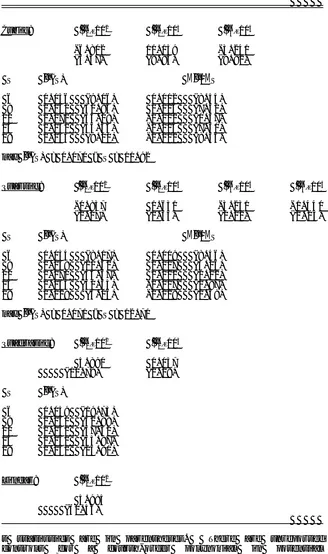
S > 0 (< 0) indicates increasing (diminishing)The results of estimating equation (7) on the full sample are
summarized at the top of Table 2. The estimated coefficients (and
their t values) on the education polynomial are reported along with
the implied estimated marginal rate of return and how it changes with
the level of schooling (and their t values). The estimated maximum
marginal rate of return and where it is reached (i.e., where returns
to scale are constant) are also reported.
The coefficient estimates on all three schooling polynomials
are highly significant. $^
2 is positive, and
$
^3 is negative. Thisindicates that at low (high) levels of schooling there are increasing
(decreasing) returns to scale in human capital production. This is
also illustrated by the estimates of the marginal rate of return at
various levels of S. D^(S) is essentially zero for the first several
years of education. It then rises at an increasing rate before
peaking at about S = 12. Then
D
^(S) begins to fall at an increasingrate. Moreover, as demonstrated by the estimates of
M
2ln(w)/M
S2, thenonlinearity is strong and highly significant (away from the gradient
peak near S = 12). The estimated change in the rate of return per
year of schooling (away from S = 12) is huge relative to the
estimates of the rate of return. Thus, constant returns to scale are
decisively rejected at low levels of education in favor of increasing
returns, and constant returns to scale are decisively rejected at
high levels of education in favor of decreasing returns. Evidently
the production function for human capital has the cubic shape of the
sort that we typically argue is ubiquitous for firms' production
functions in ECON 101.
The second set of results in Table 2 are from a fourth-order
12Similarly, Box-Cox estimates of the relationship between w and
S are extremely close to log-linearity (thus strongly suggesting near constant returns).
term. The results, however, are dramatically different when the S3
term is dropped. The relationship between ln(w) and S appears
essentially linear in the quadratic case. To capture the
nonlinearity it is essential to include the cubic term. Apparently
the distribution of increasing and decreasing returns is roughly
symmetric around the constant-returns level. Thus, in the quadratic
regression the initial increasing returns are almost exactly offset
by the later decreasing returns, hence constant returns are shown.12
This is also revealed by the quadratic estimates of
D(S) being
practically identical to the linear estimate of
D. Presumably this
is why the vast majority of previous estimates of the rate of return
are linear. A first-pass test for nonlinearity will not detect it.
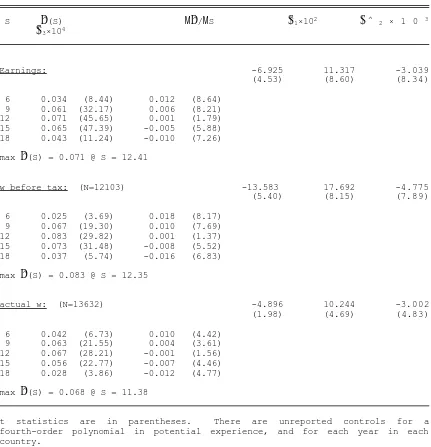
Other than this dramatic sensitivity to adding the cubic term
on schooling, the results are very robust. To show this robustness
a few additional regressions are reported in Table 3. In particular,
a cubic shape also emerges when using monthly earnings rather than
wage rates. It also emerges when using only the wage observations
which are known to be before tax (and similar results emerge when
excluding only the observations known to be after tax). Thus the
finding of a cubic shape is not due to the tax structure. The cubic
shape also emerges when using only the observations of actual
earnings (i.e., the observations with earnings measured in categories
are dropped). Hence, this source of measurement error in the wage
rate does not appear to bias the coefficient estimates.
of both tails of the schooling distribution. Card and Krueger (1992)
contend that there is a kink in an otherwise linear relationship
between log earnings and education at the education level obtained
by the second percentile of the education distribution (in 1980 U.S.
data). Thus, following Card and Krueger, the bottom two percent of
the sample (S
#
6) is removed in the regression reported at the topof Table 4. But contrary to Card and Krueger's contention, the
nonlinearity in the relationship remains. The nonlinearity also
remains when removing the top tail of the education distribution (S
$
19 is the top 2.85 percent). These two cases show that there issignificant nonlinearity at both ends of the education distribution.
In other words, there are significant increasing returns at low S,
and significant diminishing returns at high S. In fact, there is
remarkable symmetry in the returns to scale. This is further
illustrated by the quadratic regressions on the distributions above
and below the approximate constant-returns point at S = 12.
The nonlinearity between ln(w) and S is not completely driven
by the tails of the education distribution, however. The last set
of estimates in Table 4 show that when both tails are ignored, the
nonlinearity remains. The nonlinearity is reduced somewhat, but is
still statistically significant.
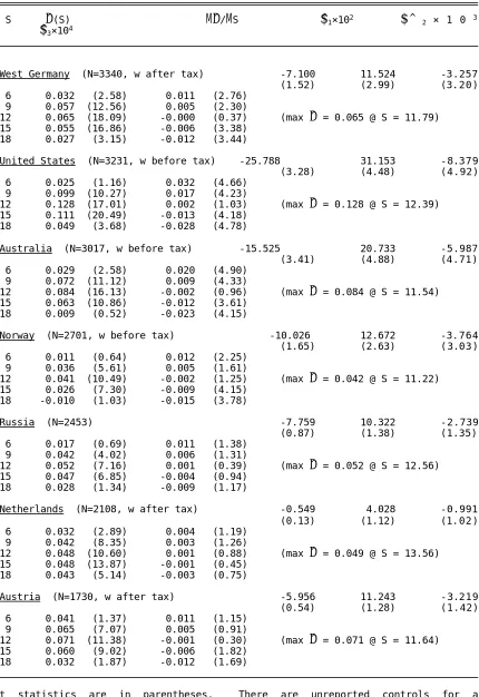
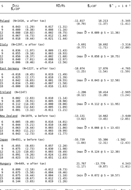
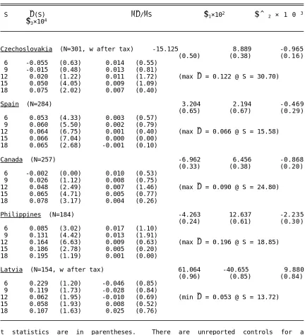
The results of estimating equation (7) on the country
subsamples are summarized in Tables 5.1 - 5.4. The same sort of
cubic shape emerges in the vast majority of cases. That is, the
coefficient estimate on S2 is positive and the coefficient estimate
on S3 is negative in 23 of the 26 cases (and statistic a l l y
significant in 10 cases). Moreover, the three opposite cases arise
13See Hungerford and Solon (1987), Card and Krueger (1992),
Jaeger and Page (1996), Harmon and Walker (1999), and Chevalier and Walker (1999).
and the three positive
$
^3 are close to being statisticallysignificant. The results for countries with the four largest samples
all show statistically significant increasing (decreasing) returns
at low (high) S.
Moreover, there is considerable similarity in the coefficient
estimates across countries, particularly those with larger sample
sizes. The similarity across countries in the estimated schooling
levels where constant returns are reached is even more remarkable.
For example, in the 13 largest samples (which all have the same signs
for
$
^2 and$
^3), the estimated constant-returns levels range between10.75 and 13.56 years of education (roughly the same amount of
variation as in mean education across countries). Moreover, there
does not appear to be systematic relationship between and the mean
S or national income. This suggests that increases in physical
capital do not raise the productivity in human capital production
enough to offset the diminishing returns.
Perhaps the more interesting source of variation in results
across countries is in
D
^(S). There is considerable variation in theestimated rate of return to education across countries. In other
words, there is more cross-country variation in the level of
D
^(S)than in the shape of D^(S).
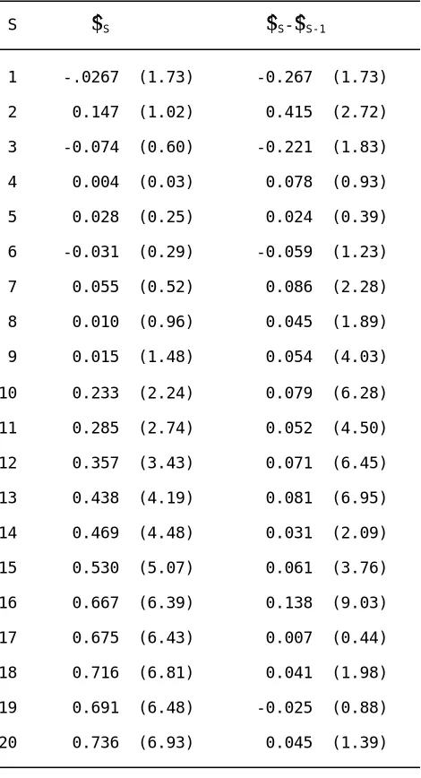
Table 6 reports the results of regressing ln(w) against a set
of dummy variables for each level of schooling. As found in several
previous studies,13 there is large amount of variation in the
14As found in Card and Krueger's (1992) data, there is a notable
kink in the rate-of-return relationship at the second percentile of the education distribution (of male workers).
15The blip at S = 16 has been found in previous studies and has
often be attributed to a "sheepskin effects".
$
^S-1). Not surprisingly, these dummy-variable results are consistent
with the results from the cubic regression. Figure 1 plots the
estimated (log) wage differential from the dummy-variable regression
along with that from the cubic regression. This figure illustrates
the estimated cubic shape of the human capital production function.
Figure 2 plots the estimated marginal rate of return from the
dummy-variable regression along with that from the cubic regression. There
is essentially no return to investment in education for at least the
first six years of school.14 Evidently, the initial increasing
returns (i.e., fixed costs) in human capital production are
substantial. And other than the upward blip at S = 16, there is
generally a downward trend in the marginal rate of return after S =
12.15
Conclusion
This study derived and estimated a very simple test for
constant returns to scale in human capital production, a crucial
assumption in dozens of recent papers on endogenous growth. The
empirical evidence is decidedly against this assumption. There is
evidence of significant decreasing returns after about the mean level
of educational attainment.
The test for constant returns - a linear relationship between
the log of the wage rate and years of education - is admittedly
hence there are a number of potential biases. On the other hand,
however, the empirical evidence is arguably overwhelming. The
evidence is so strong against constant returns that it is difficult
to imagine that it could be due to the potential biases. Moreover,
the possible biases generally work against finding diminishing
returns.
Thus, it is hard to escape the conclusion that the micro-level
evidence is unfavorable for models of endogenous growth driven by
human capital accumulation. This, of course, does not imply that
human capital is unimportant for growth. Indeed, the finding of
significant initial increasing returns suggests that human capital
accumulation may have a crucial role in development and transitional
growth.
References
Acemoglu, Daron, "A Microfoundation for Social Increasing Returns in Human Capital Accumulation," Quarterly Journal of Economics, August 1996.
Barro, Robert J., "Economic Growth in a Cross Section of Countries,"
Quarterly Journal of Economics, May 1991.
and Xavier Sala-i-Martin, "Convergence," Journal of
Political Economy, April 1992.
and , Economic Growth, McGraw-Hill, 1995.
Benhabib, Jess and Boyan Jovanovic, "Externalities and Growth Accounting," American Economic Review, March 1991.
Benhabib, Jess and Mark M. Spiegel, "The Role of Human Capital in Economic Development: Evidence from Aggregate Cross-Country Data," Journal of Monetary Economics, October 1994.
Ben-Porath, Yoram, "The Production of Human Capital over Time," in Hansen (ed.), Education, Income, and Human Capital, National Bureau of Economic Research, 1970.
Card, David, "Earnings, Schooling, and Ability Revisited," in Solomon Polachek (ed.), Research in Labor Economics, Vol. 14, 1995.
and Alan B. Krueger, "Does School Quality Matter? Returns to Education and the Characteristics of Public Schools in the
United States," Journal of Political Economy, February 1992.
Chevalier, Arnaud and Ian Walker, "Further Results on the Returns to Education in the UK," working paper, 1999.
Groot, Wim and Hessel Oosterbeek, "Earnings Effects of Different Components of Schooling; Human Capital Versus Screening,"
Review of Economics and Statistics, May 1994.
Haley, William J., "Estimation of the Earnings Profile from Optimal Human Capital Accumulation," Econometrica, November 1976.
Harmon, Colm and Ian Walker, "The Marginal and Average Returns to Schooling," European Economic Review, 1999.
Heckman, James J., "A Life-Cycle Model of Earnings, Learning, and Consumption," Journal of Political Economy, August 1976.
, Anne Layne-Farrar, and Petra Todd, "The Schooling Quality-Earnings Relationship: Using Economic Theory to Interpret Functional Forms Consistent with the Evidence," NBER Working Paper No. 5288, 1995.
Hungerford, Thomas and Gary Solon, "Sheepskin Effects in the Return to Education," Review of Economic and Statistics, February 1987.
Jaeger, David A. and Marianne E. Page, "Degrees Matter: New Evidence on Sheepskin Effects in the Returns to Education," Review of
Economics and Statistics, November 1996.
Jones, Charles I., "Time Series Tests of Endogenous Growth Models,"
Quarterly Journal of Economics, May 1995.
Jones, Larry E., Rodolfo E. Manuelli, and Peter E. Rossi, "Optimal Taxation in Models of Endogenous Growth," Journal of Political
Economy, June 1993.
Kroch, Eugene A. and Kriss Sjoblom, "Schooling as Human Capital or a Signal," Journal of Human Resources, Winter 1994.
King, Robert G. and Sergio Rebelo, "Public Policy and Economic Growth: Developing Neoclassical Implications," Journal of
Political Economy, October 1990.
September 1992.
Levine, Ross and Sara J. Zervos, "What We Have Learned About Policy and Growth from Cross-Country Regressions?" American Economic
Review, May 1993.
Lucas, Robert E., Jr., "On the Mechanics of Economic Development,"
Journal of Monetary Economics, July 1988.
Mankiw, N. Gregory, David Romer, and David N. Weil, "A Contribution to the Empirics of Economic Growth," Quarterly Journal of
Economics, May 1992.
Mulligan, Casey B. and Xavier Sala-i-Martin, "Transitional Dynamics in Two-Sector Models of Endogenous Growth," Quarterly Journal
of Economics, August 1993.
Murphy, Kevin M. and Finis Welch, "Empirical Age-Earnings Profiles,"
Journal of Labor Economics, April 1990.
Pack, Howard, "Endogenous Growth Theory: Intellectual Appeal and Empirical Shortcomings," Journal of Economic Perspectives, Winter 1994.
Park, Jin Heum, "Estimation of Sheepskin Effects Using the Old and New Measures of Educational Attainment in the Consumer Population Survey," Economics Letters, 1999.
Psacharopoulos, George, "Returns to Education: A Further International Update and Implications," Journal of Human
Resources, 1985.
, "Returns to Investment in Education: A Global Update,"
World Development, 1994.
Rebelo, Sergio, "Long-Run Policy Analysis and Long-Run Growth,"
Journal of Political Economy, June 1991.
Romer, Paul M., "Human Capital and Growth: Theory and Evidence,"
Carnegie-Rochester Conference Series on Public Policy, 1990.
, "The Origins of Endogenous Growth,"Journal of Economic
Perspectives," Winter 1994.
Rosen, Sherwin, "A Theory of Life Earnings," Journal of Political
Economy, August 1976.
Saint-Paul, Gilles, "Unemployment and Increasing Private Returns to Human Capital," Journal of Public Economics, July 1996.
Tallman, Ellis W. and Ping Wang, "Human Capital and Endogenous Growth: Evidence from Taiwan," Journal of Monetary Economics, August 1994.
Weiss, Andrew, "Human Capital vs. Signalling Explanations of Wages,"
Journal of Economic Perspectives, Fall 1995.
Country N S6 sS Tax
All 30607 12.03 3.18
West Germany 3340 10.45 2.93 after
United States 3231 13.55 2.90 before
Australia 3017 11.65 2.77 before
Norway 2701 12.47 2.90 before
Russia 2453 13.05 3.37 ?
Netherlands 2200 12.94 3.49 after
Austria 1892 10.98 2.44 after
Poland 1416 11.02 2.63 after
Italy 1297 11.77 3.81 after
East Germany 1227 10.88 2.87 after
Ireland 1189 11.99 2.95 **
New Zealand 1079 12.63 3.03 before
Japan 851 12.85 2.63 before
Hungary 649 11.45 2.72 after
Sweden 600 11.81 3.39 before
Slovenia 586 11.10 2.75 after
Israel 483 12.69 2.94 ?
Czech Republic 462 13.04 2.67 after
Bulgaria 377 11.56 3.03 ?
Slovak Republic 368 12.43 2.41 ?
Switzerland 305 10.76 3.33 after
Czechoslovakia 301 12.80 2.52 after
Spain 284 10.62 4.28 ?
Canada 257 15.01 3.14 ?
Philippines 184 9.55 4.06 ?
Latvia 154 12.51 3.07 after
[image:22.596.119.477.95.743.2]
Cubic: $^1×10² $^2×10³ $^3×10⁴
-6.802 11.159 -3.241 (4.47) (8.84) (8.92)
S D^(S) MD^/MS
6 0.036 (9.06) 0.012 (8.54) 9 0.062 (32.93) 0.006 (7.51) 12 0.070 (45.18) -0.000 (0.37) 15 0.061 (44.44) -0.006 (7.50) 18 0.034 (9.00) -0.012 (8.46) max D^(S) = 0.070 @ S = 11.92
Quartic: $^1×10² $^2×10³ $^3×10⁴ $^4×10⁵
-0.837 1.631 -3.231 -1.440 (0.27) (0.35) (1.11) (2.24)
S D^(S) MD^/MS
6 0.034 (8.17) 0.009 (8.46) 9 0.058 (21.42) 0.007 (3.16) 12 0.071 (44.67) 0.002 (2.22) 15 0.064 (31.43) -0.007 (1.87) 18 0.029 (6.26) -0.018 (1.69) max D^(S) = 0.071 @ S = 12.71
Quadratic: $^1×10² $^2×10³
5.890 0.037 (10.79) (0.18)
S D^(S)
6 0.059 (19.73) 9 0.060 (31.98) 12 0.060 (57.62) 15 0.060 (43.87) 18 0.060 (24.90)
Linear: $^1×10²
5.985 (60.56)
[image:23.596.135.463.93.647.2]
S D^(S) MD^/MS $^1×10² $^ 2 × 1 0 3 $^3×10⁴
Earnings: -6.925 11.317 -3.039
(4.53) (8.60) (8.34)
6 0.034 (8.44) 0.012 (8.64) 9 0.061 (32.17) 0.006 (8.21) 12 0.071 (45.65) 0.001 (1.79) 15 0.065 (47.39) -0.005 (5.88) 18 0.043 (11.24) -0.010 (7.26) max D^(S) = 0.071 @ S = 12.41
w before tax: (N=12103) -13.583 17.692 -4.775 (5.40) (8.15) (7.89)
6 0.025 (3.69) 0.018 (8.17) 9 0.067 (19.30) 0.010 (7.69) 12 0.083 (29.82) 0.001 (1.37) 15 0.073 (31.48) -0.008 (5.52) 18 0.037 (5.74) -0.016 (6.83) max D^(S) = 0.083 @ S = 12.35
actual w: (N=13632) -4.896 10.244 -3.002 (1.98) (4.69) (4.83)
6 0.042 (6.73) 0.010 (4.42) 9 0.063 (21.55) 0.004 (3.61) 12 0.067 (28.21) -0.001 (1.56) 15 0.056 (22.77) -0.007 (4.46) 18 0.028 (3.86) -0.012 (4.77) max D^(S) = 0.068 @ S = 11.38
[image:24.596.83.514.93.540.2]
S D^(S) MD^/MS $^1×10² $^ 2 × 1 0 3 $^3×10⁴
S $ 7: (N=29999) -12.086 1 5 . 6 1 6 -4.223
(3.10) (5.16) (5.58)
6 0.021 (1.88) 0.016 (4.79) 9 0.058 (16.14) 0.008 (4.18) 12 0.071 (40.01) 0.001 (1.03) 15 0.063 (36.33) -0.007 (7.02) 18 0.031 (6.90) -0.014 (6.47) max D^(S) = 0.072 @ S = 12.33
S # 18: (N=29735) -4.923 9.456 -2.512 (2.83) (5.87) (5.24)
6 0.037 (9.23) 0.010 (6.40) 9 0.060 (28.91) 0.005 (6.87) 12 0.069 (41.67) 0.001 (1.46) 15 0.065 (32.84) -0.004 (2.98) 18 0.047 (7.41) -0.008 (4.00) max D^(S) = 0.069 @ S = 12.55
S $ 12: (N=16579) 19.801 -4.531 (8.47) (5.90)
12 0.089 (17.17) 15 0.062 (34.38) 18 0.035 (7.45)
S # 12: (N=19142) -3.375 5.362 (2.80) (8.10)
6 0.031 (6.75) 9 0.063 (26.97) 12 0.095 (20.31)
7 # S # 18: (N=29127) -5.099 9.593 -2.544 (0.94) (2.15) (2.15)
6 0.037 (2.61) 0.010 (2.14) 9 0.060 (16.01) 0.005 (2.09) 12 0.069 (30.32) 0.001 (1.08) 15 0.065 (32.53) -0.004 (1.97) 18 0.047 (4.99) -0.008 (2.10) max D^(S) = 0.070 @ S = 12.57
[image:25.596.87.512.90.705.2]
S D^(S) MD^/MS $^1×10² $^ 2 × 1 0 3 $^3×10⁴
West Germany (N=3340, w after tax) -7.100 11.524 -3.257 (1.52) (2.99) (3.20) 6 0.032 (2.58) 0.011 (2.76)
9 0.057 (12.56) 0.005 (2.30)
12 0.065 (18.09) -0.000 (0.37) (max D^ = 0.065 @ S = 11.79) 15 0.055 (16.86) -0.006 (3.38)
18 0.027 (3.15) -0.012 (3.44)
United States (N=3231, w before tax) -25.788 31.153 -8.379 (3.28) (4.48) (4.92) 6 0.025 (1.16) 0.032 (4.66)
9 0.099 (10.27) 0.017 (4.23)
12 0.128 (17.01) 0.002 (1.03) (max D^ = 0.128 @ S = 12.39) 15 0.111 (20.49) -0.013 (4.18)
18 0.049 (3.68) -0.028 (4.78)
Australia (N=3017, w before tax) -15.525 20.733 -5.987 (3.41) (4.88) (4.71) 6 0.029 (2.58) 0.020 (4.90)
9 0.072 (11.12) 0.009 (4.33)
12 0.084 (16.13) -0.002 (0.96) (max D^ = 0.084 @ S = 11.54) 15 0.063 (10.86) -0.012 (3.61)
18 0.009 (0.52) -0.023 (4.15)
Norway (N=2701, w before tax) -10.026 12.672 -3.764 (1.65) (2.63) (3.03) 6 0.011 (0.64) 0.012 (2.25)
9 0.036 (5.61) 0.005 (1.61)
12 0.041 (10.49) -0.002 (1.25) (max D^ = 0.042 @ S = 11.22) 15 0.026 (7.30) -0.009 (4.15)
18 -0.010 (1.03) -0.015 (3.78)
Russia (N=2453) -7.759 10.322 -2.739
(0.87) (1.38) (1.35) 6 0.017 (0.69) 0.011 (1.38)
9 0.042 (4.02) 0.006 (1.31)
12 0.052 (7.16) 0.001 (0.39) (max D^ = 0.052 @ S = 12.56) 15 0.047 (6.85) -0.004 (0.94)
18 0.028 (1.34) -0.009 (1.17)
Netherlands (N=2108, w after tax) -0.549 4.028 -0.991 (0.13) (1.12) (1.02) 6 0.032 (2.89) 0.004 (1.19)
9 0.042 (8.35) 0.003 (1.26)
12 0.048 (10.60) 0.001 (0.88) (max D^ = 0.049 @ S = 13.56) 15 0.048 (13.87) -0.001 (0.45)
18 0.043 (5.14) -0.003 (0.75)
Austria (N=1730, w after tax) -5.956 11.243 -3.219 (0.54) (1.28) (1.42) 6 0.041 (1.37) 0.011 (1.15)
9 0.065 (7.07) 0.005 (0.91)
12 0.071 (11.38) -0.001 (0.30) (max D^ = 0.071 @ S = 11.64) 15 0.060 (9.02) -0.006 (1.82)
18 0.032 (1.87) -0.012 (1.69)
[image:26.596.83.513.96.722.2]
S D^(S) MD^/MS $^1×10² $^ 2 × 1 0 3 $^3×10⁴
Poland (N=1416, w after tax) -11.817 18.213 -5.345 (0.79) (1.37) (1.41) 6 0.043 (1.29) 0.017 (1.31)
9 0.080 (8.38) 0.008 (1.16)
12 0.088 (10.02) -0.002 (0.75) (max D^ = 0.089 @ S = 11.36) 15 0.067 (6.73) -0.012 (1.44)
18 0.018 (0.44) -0.021 (1.44)
Italy (N=1297, w after tax) -5.691 10.692 -3.316 (0.77) (1.71) (2.00) 6 0.036 (1.97) 0.009 (1.43)
9 0.055 (9.10) 0.003 (0.93)
12 0.056 (8.37) -0.002 (1.68) (max D^ = 0.058 @ S = 10.75) 15 0.040 (7.01) -0.008 (2.97)
18 0.006 (0.46) -0.014 (2.56)
East Germany (N=1227, w after tax) -18.074 17.876 -4.765 (1.25) (1.54) (1.59) 6 -0.018 (0.45) 0.019 (1.49)
9 0.025 (2.17) 0.010 (1.39)
12 0.042 (6.65) 0.001 (0.55) (max D^ = 0.043 @ S = 12.50) 15 0.034 (5.69) -0.007 (1.58)
18 -0.000 (0.00) -0.016 (1.63)
Ireland (N=1147) -1.206 10.414 -2.905
(0.12) (1.20) (1.24) 6 0.082 (2.83) 0.010 (1.14)
9 0.105 (8.91) 0.005 (0.98)
12 0.112 (14.19) -0.000 (0.00) (max D^ = 0.112 @ S = 11.95) 15 0.104 (12.64) -0.005 (1.09)
18 0.081 (3.32) -0.011 (1.21)
New Zealand (N=1079, w before tax) -13.131 14.662 -3.640 (3.02) (3.45) (2.85) 6 0.005 (0.49) 0.016 (4.01)
9 0.044 (5.21) 0.010 (4.68)
12 0.063 (8.44) 0.003 (1.86) (max D^ = 0.066 @ S = 13.43) 15 0.063 (11.21) -0.003 (0.99)
18 0.043 (2.73) -0.010 (1.77)
Japan (N=851, w before tax) -55.739 55.386 -1.502 (1.84) (2.31) (2.43) 6 -0.055 (0.65) 0.057 (2.20)
9 0.075 (2.73) 0.030 (1.98)
12 0.123 (10.45) 0.003 (0.49) (max D^ = 0.124 @ S = 12.30) 15 0.091 (9.26) -0.024 (2.69)
18 -0.023 (0.51) -0.051 (2.63)
Hungary (N=649, w after tax) 21.767 -13.770 4.343 (1.17) (0.87) (1.01) 6 0.099 (2.18) -0.012 (0.73)
9 0.075 (5.58) -0.004 (0.46)
12 0.075 (6.44) 0.004 (1.10) (min D^ = 0.072 @ S = 10.57) 15 0.098 (8.67) 0.012 (1.45)
18 0.144 (3.65) 0.019 (1.26)
[image:27.596.83.514.94.719.2]
S D^(S) MD^/MS $^1×10² $^ 2 × 1 0 3 $^3×10⁴
Sweden (N=600, w before tax) -3.994 8.217 -2.496 (0.92) (2.01) (2.05) 6 0.032 (3.01) 0.007 (1.89)
9 0.047 (6.91) 0.003 (1.45)
12 0.049 (8.42) -0.002 (0.98) (max D^ = 0.005 @ S = 10.97) 15 0.038 (7.24) -0.006 (1.88)
18 0.013 (0.86) -0.011 (2.00)
Slovenia (N=586, w after tax) -34.558 36.657 -9.571 (2.71) (2.95) (2.51) 6 -0.009 (0.39) 0.039 (3.42)
9 0.081 (6.87) 0.022 (4.19)
12 0.120 (10.54) 0.004 (1.01) (max D^ = 0.122 @ S = 12.76) 15 0.108 (6.01) -0.012 (1.25)
18 0.043 (0.79) -0.030 (1.78)
Israel (N=483) -26.324 30.432 -8.351 (3.30) (4.21) (4.01) 6 0.012 (0.56) 0.031 (4.28)
9 0.082 (6.29) 0.016 (4.04)
12 0.106 (9.79) 0.001 (0.28) (max D^ = 0.106 @ S = 12.15) 15 0.086 (10.45) -0.014 (2.77)
18 0.021 (0.88) -0.029 (3.39)
Czech Republic (N=462, w after tax) -6.289 9.250 -2.537 (0.46) (0.84) (0.87) 6 0.021 (0.53) 0.009 (0.80)
9 0.042 (2.37) 0.005 (0.70)
12 0.050 (4.15) 0.002 (0.00) (max D^ = 0.050 @ S = 12.16) 15 0.043 (5.56) -0.004 (0.77)
18 0.024 (0.96) -0.009 (0.87)
Bulgaria (N=377) -4.929 8.281 -2.182
(0.66) (1.11) (0.93) 6 0.027 (1.38) 0.009 (1.27)
9 0.047 (3.11) 0.005 (1.35)
12 0.055 (4.48) 0.001 (0.22) (max D^ = 0.055 @ S = 12.65) 15 0.052 (3.90) -0.003 (0.44)
18 0.037 (1.02) -0.007 (0.63)
Slovak Republic (N=368) 4.467 0.986 -0.452 (0.18) (0.05) (0.09) 6 0.052 (0.77) 0.000 (0.00)
9 0.051 (2.41) -0.000 (0.00)
12 0.049 (3.61) -0.001 (0.28) (max D^ = 0.052 @ S = 7.26) 15 0.044 (4.45) -0.002 (0.28)
18 0.036 (1.05) -0.003 (0.05)
Switzerland (N= 305, w after tax) 20.296 -8.443 1.783 (2.09) (0.96) (0.69) 6 0.121 (4.70) -0.010 (1.20)
9 0.094 (6.24) -0.007 (1.52)
12 0.077 (6.51) -0.004 (1.13) (min D^ = 0.070 @ S = 15.78) 15 0.070 (6.17) -0.001 (0.14)
18 0.072 (2.21) 0.002 (0.22)
[image:28.596.83.513.88.725.2]
S D^(S) MD^/MS $^1×10² $^ 2 × 1 0 3 $^3×10⁴
Czechoslovakia (N=301, w after tax) -15.125 8.889 -0.965 (0.50) (0.38) (0.16) 6 -0.055 (0.63) 0.014 (0.55)
9 -0.015 (0.48) 0.013 (0.81)
12 0.020 (1.22) 0.011 (1.72) (max D^ = 0.122 @ S = 30.70) 15 0.050 (4.05) 0.009 (1.09)
18 0.075 (2.02) 0.007 (0.40)
Spain (N=284) 3.204 2.194 -0.469
(0.65) (0.67) (0.29) 6 0.053 (4.33) 0.003 (0.57)
9 0.060 (5.50) 0.002 (0.79)
12 0.064 (6.75) 0.001 (0.40) (max D^ = 0.066 @ S = 15.58) 15 0.066 (7.04) 0.000 (0.00)
18 0.065 (2.68) -0.001 (0.10)
Canada (N=257) -6.962 6.456 -0.868
(0.33) (0.38) (0.20) 6 -0.002 (0.00) 0.010 (0.53)
9 0.026 (1.12) 0.008 (0.75)
12 0.048 (2.49) 0.007 (1.46) (max D^ = 0.090 @ S = 24.80) 15 0.065 (4.71) 0.005 (0.77)
18 0.078 (3.17) 0.004 (0.26)
Philippines (N=184) -4.263 12.637 -2.235 (0.24) (0.61) (0.30) 6 0.085 (3.02) 0.017 (1.10)
9 0.131 (4.42) 0.013 (1.91)
12 0.164 (6.63) 0.009 (0.63) (max D^ = 0.196 @ S = 18.85) 15 0.186 (2.78) 0.005 (0.20)
18 0.195 (1.19) 0.001 (0.00)
Latvia (N=154, w after tax) 61.064 -40.655 9.880 (0.96) (0.85) (0.84) 6 0.229 (1.20) -0.046 (0.85)
9 0.119 (1.73) -0.028 (0.84)
12 0.062 (1.95) -0.010 (0.69) (min D^ = 0.053 @ S = 13.72) 15 0.058 (1.93) 0.008 (0.52)
18 0.107 (1.63) 0.025 (0.76)
[image:29.596.82.514.93.568.2]
S $^S $^S-$^S-1
1 -.0267 (1.73) -0.267 (1.73)
2 0.147 (1.02) 0.415 (2.72)
3 -0.074 (0.60) -0.221 (1.83)
4 0.004 (0.03) 0.078 (0.93)
5 0.028 (0.25) 0.024 (0.39)
6 -0.031 (0.29) -0.059 (1.23)
7 0.055 (0.52) 0.086 (2.28)
8 0.010 (0.96) 0.045 (1.89)
9 0.015 (1.48) 0.054 (4.03)
10 0.233 (2.24) 0.079 (6.28)
11 0.285 (2.74) 0.052 (4.50)
12 0.357 (3.43) 0.071 (6.45)
13 0.438 (4.19) 0.081 (6.95)
14 0.469 (4.48) 0.031 (2.09)
15 0.530 (5.07) 0.061 (3.76)
16 0.667 (6.39) 0.138 (9.03)
17 0.675 (6.43) 0.007 (0.44)
18 0.716 (6.81) 0.041 (1.98)
19 0.691 (6.48) -0.025 (0.88)
20 0.736 (6.93) 0.045 (1.39)
[image:30.596.181.416.100.534.2]