A Probabilistic Model for Canonicalizing Named Entity Mentions
Dani Yogatama Yanchuan Sim Noah A. Smith Language Technologies Institute
Carnegie Mellon University Pittsburgh, PA 15213, USA
{dyogatama,ysim,nasmith}@cs.cmu.edu
Abstract
We present a statistical model for canonicalizing named entity mentions into a table whose rows rep-resent entities and whose columns are attributes (or parts of attributes). The model is novel in that it incorporates entity context, surface features, first-order dependencies among attribute-parts, and a no-tion of noise. Transductive learning from a few seeds and a collection of mention tokens combines Bayesian inference and conditional estimation. We evaluate our model and its components on two datasets collected from political blogs and sports news, finding that it outperforms a simple agglom-erative clustering approach and previous work.
1 Introduction
Proper handling of mentions in text of real-world entities—identifying and resolving them—is a cen-tral part of many NLP applications. We seek an al-gorithm that infers a set of real-world entities from mentions in a text, mapping each entity mention to-ken to an entity, and discovers general categories of words used in names (e.g., titles and last names). Here, we use a probabilistic model to infer a struc-tured representation of canonical forms of entity at-tributes through transductive learning from named entity mentions with a small number of seeds (see Table 1). The input is a collection of mentions found by a named entity recognizer, along with their con-texts, and, following Eisenstein et al. (2011), the output is a table in which entities are rows (the num-ber of which is not pre-specified) and attribute words are organized into columns.
This paper contributes a model that builds on the approach of Eisenstein et al. (2011), but also:
• incorporates context of the mention to help with disambiguation and to allow mentions that do not share words to be merged liberally;
• conditions against shape features, which improve the assignment of words to columns;
• is designed to explicitly handle some noise; and
• is learned using elements of Bayesian inference with conditional estimation (see§2).
We experiment with variations of our model, comparing it to a baseline clustering method and the model of Eisenstein et al. (2011), on two datasets, demonstrating improved performance over both at recovering a gold standard table. In a political blogs dataset, the mentions refer to political fig-ures in the United States (e.g., Mrs. Obama and Michelle Obama). As a result, the model discov-ers parts of names—hMrs., Michelle, Obamai— while simultaneously performing coreference res-olution for named entity mentions. In the sports news dataset, the model is provided with named en-tity mentions of heterogenous types, and success here consists of identifying the correct team for ev-ery player (e.g.,Kobe BryantandLos Angeles Lak-ers). In this scenario, given a few seed examples, the model begins to identify simple relations among named entities (in addition to discovering attribute structures), since attributes are expressed as named entities across multiple mentions. We believe this adaptability is important, as the salience of different kinds of names and their usages vary considerably across domains.
Bill Clinton Mr.
George Bush Mr. W.
Barack Obama Sen. Hussein Hillary Clinton Mrs. Sen.
Bristol Palin Ms.
Emil Jones Jr.
Kay Hutchison Bailey
Ben Roethlisberger Steelers Bryant Los Angeles
Derek Jeter New York
Table 1: Seeds for politics (above) and sports (below).
[image:1.612.314.539.544.666.2]x ↵
1
1
f
w c
r s ✓
⌘ ⌧
M L
T
[image:2.612.87.291.60.242.2]µ C
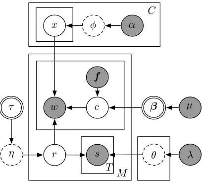
Figure 1: Graphical representation of our model. Top, the generation of the table: C is the number of at-tributes/columns, the number of rows is infinite,α is a vector of concentration parameters,φ is a multinomial distribution over strings, andxis a word in a table cell. Lower left, for choosing entities to be mentioned:τ deter-mines the stick lengths andη is the distribution over en-tities to be selected for mention. Middle right, for choos-ing attributes to use in a mention:f is the feature vector, andβis the weight vector drawn from a Laplace distri-bution with mean zero and varianceµ. Center, for gen-erating mentions: M is the number of mentions in the data,wis a word token set from an entity/rowrand at-tribute/columnc. Lower right, for generating contexts:s is a context word, drawn from a multinomial distribution θwith a Dirichlet priorλ. Variables that are known or fixed are shaded; variables that are optimized are double circled. Others are latent; dashed lines imply collapsing.
2 Model
We begin by assuming as input a set of mention to-kens, each one or more words. In our experiments these are obtained by running a named entity recog-nizer. The output is a table in which rows are un-derstood to correspond to entities (types, not men-tion tokens) and columns are fields, each associated with an attribute or a part of it. Our approach is based on a probabilistic graphical model that gener-ates the mentions, which are observed, and the table, which is mostly unobserved, similar to Eisenstein et al. (2011). Our learning procedure is a hybrid of Bayesian inference and conditional estimation. The generative story, depicted in Figure 1, is:
• For each columnj∈ {1, . . . , C}:
◦ Draw a multinomial distribution φj over the
vocabulary from a Dirichlet process: φj ∼
DP(αj, G0). This is the lexicon for fieldj. ◦ Generate table entries. For each rowi(of which
there are infinitely many), draw an entry xi,j for celli, jfromφj. A few of these entries (the seeds) are observed; we denote thosex˜.
◦ Draw weightsβj that associate shape and po-sitional features with columns from a 0-mean,
µ-variance Laplace distribution.
• Generate the distribution over entities to be men-tioned in general text: η ∼ GEM(τ) (“stick-breaking” distribution).
• Generate context distributions. For each rowr:
◦ Draw a multinomial over the context vocabu-lary (distinct from mention vocabuvocabu-lary) from a Dirichlet distribution,θr∼Dir(λ).
• For each mention tokenm:
◦ Draw an entity/rowr ∼η.
◦ For each word in the mentionw, given some of its featuresf (assumed observed):
. Choose a column c ∼ Z1 exp(β>cf). This uses a log-linear distribution with partition function Z. In one variation of our model, first-order dependencies among the columns are enabled; these introduce a dynamic char-acter to the graphical model that is not shown in Figure 1.
. With probability 1−, set the textwm` to bexrc. Otherwise, generate any word from a unigram-noise distribution.
◦ Generate mention context. For each of theT = 10context positions (five before and five after the mention), draw the wordsfromθr.
Our choices of prior distributions reflect our be-liefs about the shapes of the various distributions. We expect field lexicons φj and the distributions over mentioned entitiesηto be “Zipfian” and so use tools from nonparametric statistics to model them. We expect column-feature weights β to be mostly zero, so a sparsity-inducing Laplace prior is used (Tibshirani, 1996).
Our goal is to maximize the conditional likeli-hood of most of the evidence (mentions, contexts, and seeds),p(w, s,x˜|α,β, λ, τ, µ, ,f) =
P
r
P
c
P
x\x˜
R
dθR
dηR
dφ
with respect toβandτ. We fixα(see§3.3 for the values ofαfor each dataset),λ = 2(equivalent to add-one smoothing), µ = 2×10⁻⁸, = 10−10, and each mention word’sf. Fixingλ,µ, andα is essentially just “being Bayesian,” or fixing a hyper-parameter based on prior beliefs. Fixingf is quite different; it is conditioning our model on some ob-servable features of the data, in this case word shape features. We do this to avoid integrating over fea-ture vector values. These choices highlight that the design of a probabilistic model can draw from both Bayesian and discriminative tools. Observing some ofxas seeds (x˜) renders this approach transductive. Exact inference in this model is intractable, so we resort to an approximate inference technique based on Markov Chain Monte Carlo simulation. The opti-mization ofβcan be described as “contrastive” esti-mation (Smith and Eisner, 2005), in which some as-pects of the data are conditioned against for compu-tational convenience. The optimization ofτ can be described as “empirical Bayesian” estimation (Mor-ris, 1983) in which the parameters of a prior are fit to data. Our overall learning procedure is a Monte Carlo Expectation Maximization algorithm (Wei and Tanner, 1990).
3 Learning and Inference
Our learning procedure is an iterative algorithm con-sisting of two steps. In the E-step, we perform col-lapsed Gibbs sampling to obtain distributions over row and column indices for every mention, given the current value of the hyperparamaters. In the M-step, we obtain estimates for the hyperparameters, given the current posterior distributions.
3.1 E-step
For themth mention, we sample row indexr, then for each wordwm`, we sample column indexc.
3.1.1 Sampling Rows
Similar to Eisenstein et al. (2011), when we sam-ple the row for a mention, we use Bayes’ rule and marginalize the columns. We further incorporate context information and a notion of noise.
p(rm =r|. . .)∝p(rm =r|r−m, η)
(Q
`
P
cp(wm` |x, rm=r, cm` =c))
(Q
tp(smt|rm=r))
We consider each quantity in turn.
Prior. The probability of drawing a row index
fol-lows a stick breaking distribution. This alfol-lows us to have an unbounded number of rows and let the model infer the optimal value from data. A standard marginalization ofηgives us:
p(rm=r |r−m, τ) =
(
Nr−m N+τ ifN
−m r >0 τ
N+τ otherwise,
whereN is the number of mentions,Nris the num-ber of mentions assigned to rowr, andNr−mis the number of mentions assigned to rowr, excludingm.
Mention likelihood. In order to compute the
likeli-hood of observing mentions in the dataset, we have to consider a few cases. If a cell in a table has al-ready generated a word, it can only generate that word. This hard constraint was a key factor in the inference algorithm of Eisenstein et al. (2011); we speculate that softening it may reduce MCMC mix-ing time, so introduce a notion of noise. With proba-bility= 10−10, the cell can generate any word. If a cell has not generated any word, its probability still depends on other elements of the table. With base distributionG0,1and marginalizingφ, we have:
p(wm`|x, rm=r, cm`=c, αc) = (1)
1− ifxrc =wm`
ifxrc 6∈ {wm`,∅}
Ncw−m` Nc−m`+αc
ifxrc =∅andNcw >0
G0(wm`)N−m`αc c +αc
ifxrc =∅andNcw = 0
whereNc−m`is the number of cells in columncthat are not empty andNcw−m` is the number of cells in columncthat are set to the wordwm`; both counts excluding the current word under consideration.
Context likelihood. It is important to be able to
use context information to determine which row a mention should go into. As a novel extension, our model also uses surrounding words of a mtion as its “context”—similar context words can en-courage two mentions that do not share any words to be merged. We choose a Dirichlet-multinomial distribution for our context distribution. For every row in the table, we have a multinomial distribution over context vocabularyθrfrom a Dirichlet priorλ.
1
Therefore, the probability of observing thetth con-text word for mentionmisp(smt|rm =r, λ)
=
( N−mt
rs +λs−1 Nr−mt+
P vλv−V
ifNr−mt>0
λs−1
P vλv−V
otherwise,
whereNr−mtis the number of context words of men-tions assigned to rowr,Nrs−mtis the number of con-text words of mentions assigned to row r that are
smt, both excluding the current context word, andv ranges over the context vocabulary of sizeV.
3.1.2 Sampling Columns
Our column sampling procedure is novel to this work and substantially differs from that of Eisen-stein et al. (2011). First, we note that when we sam-ple column indices for each word in a mention, the row index for the mentionr has already been sam-pled. Also, our model has interdependencies among column indices of a mention.2 Standard Gibbs sam-pling procedure breaks down these dependencies. For faster mixing, we experiment with first-order dependencies between columns when sampling col-umn indices. This idea was suggested by Eisenstein et al. (2011, footnote 1) as a way to learn structure in name conventions. We suppressed this aspect of the model in Figure 1 for clarity.
We sample the column indexc1 for the first word
in the mention, marginalizing out probabilities of other words in the mention. After we sample the column index for the first word, we sample the col-umn index c2 for the second word, fixing the pre-vious word to be in column c1, and marginalizing
out probabilities ofc3, . . . , cLas before. We repeat the above procedure until we reach the last word in the mention. In practice, this can be done effi-ciently using backward probabilities computed via dynamic programming. This kind of blocked Gibbs sampling was proposed by Jensen et al. (1995) and used in NLP by Mochihashi et al. (2009). We have:
p(cm`=c|. . .)∝
p(cm`=c|fm`, β)p(cm`=c|cm`− =c−)
P
c+pb(cm` =c|cm`+ =c+)
p(wm` |x, rm=r, cm` =c, αc),
2As shown in Figure 1, column indices in a mention form
“v-structures” with the row indexr. Since everyw`is observed, there is an active path that goes through all these nodes.
where`− is the preceding word andc− is its
sam-pled index, `+ is the following word andc+ is its
possible index, andpb(·)are backward probabilities. Alternatively, we can perform standard Gibbs sam-pling and drop the dependencies between columns, which makes the model rely more heavily on the fea-tures. For completeness, we detail the computations.
Featurized log linear distribution. Our model can
use arbitrary features to choose a column index. These features are incorporated as a log-linear
dis-tribution,p(cm` = c | fm`,β) =
exp(β>cfm`) P
c0exp(β > c0fm`)
.
The list of features used in our experiments is: 1{w is the first word in the mention}; 1{w ends with a period}; 1{w is the last word in the men-tion}; 1{w is a Roman numeral}; 1{w starts with an upper-case letter}; 1{w is an Arabic number}; 1{w ∈ {mr,mrs,ms,miss,dr,mdm} }; 1{w con-tains ≥ 1 punctuation symbol}; 1{w ∈ {jr,sr}}; 1{w ∈ {is,in,of,for}}; 1{w is a person entity}; 1{wis an organization entity}.
Forward and backward probabilities. Since
we introduce first-order dependencies between columns, we have forward and backward probabili-ties, as in HMMs. However, we always sample from left to right, so we do not need to marginalize ran-dom variables to the left of the current variable be-cause their values are already sampled. Our transi-tion probabilities are as follows:
p(cm` =c|cm`−=c−) =
Nc−−m,c P
c0−N
−m
c0−,c
,
whereNc−−m,cis the number of times we observe tran-sitions from columnc− toc, excluding mentionm.
The forward and backward equations are simple (we omit them for space).
Mention likelihood. Mention likelihood p(wm` |
x, rm = r, cm` = c, αc) is identical to when we sample the row index (Eq. 1).
3.2 M-step
3.3 Implementation Details
We ran Gibbs sampling for 500 iterations,3 discard-ing the first 200 for burn-in and averagdiscard-ing counts over every 10th sample to reduce autocorrelation.
For each word in a mentionw, we introduced 12 binary featuresffor our featurized log-linear distri-bution (§3.1.2).
We then downcased all words in mentions for the purpose of defining the table and the mention words
w. Ten context words (5 each to the left and right) definesfor each mention token.
For non-convex optimization problems like ours, initialization is important. To guide the model to reach a good local optimum without many restarts, we manually initialized feature weights and put a prior on transition probabilities to reflect phenom-ena observed in the initial seeds. The initializer was constructed once and not tuned across experiments.4 The M-step was performed every 50 Gibbs sampling iterations. After inference, we filled each cell with the word that occurred at least80%of the time in the averaged counts for the cell, if such a word existed.
4 Experiments
We compare several variations of our model to Eisenstein et al. (2011) (the authors provided their implementation to us) and a clustering baseline.
4.1 Datasets
We collected named entity mentions from two cor-pora: political blogs and sports news. The political blogs corpus is a collection of blog posts about poli-tics in the United States (Eisenstein and Xing, 2010), and the sports news corpus contains news summaries of major league sports games (National Basketball
3
On our moderate-sized datasets (see§4.1), each iteration takes approximately three minutes on a 2.2GHz CPU.
4
For the politics dataset, we set C = 6, α =
h1.0,1.0,10−12,10−15,10−12,10−8i, initializedτ = 1, and used a Dirichlet prior on transition counts such that before ob-serving any data:N0,1 = 10, N0,5 = 5, N2,0 = 10, N2,1 =
10, N2,3 = 10, N2,4 = 5, N3,0 = 10, N3,1 = 10, N5,1 = 15
(others are set to zero). For the sports dataset, we setC = 5, α = h1.0,1.0,10−15,10−6,10−6i, initializedτ = 1, and
used a Dirichlet prior on transition countsN0,1 = 10, N2,3 =
20, N3,4= 10(others are set to zero). We also manually
initial-ized the weights of some featuresβfor both datasets. These val-ues were obtained from preliminary experiments on a smaller sample of the datasets, and updated on the first EM iteration.
[image:5.612.332.520.61.128.2]Politics Sports # source documents 3,000 700 # mentions 10,647 13,813 # unique mentions 528 884 size of mention vocabulary 666 1,177 size of context vocabulary 2,934 2,844
Table 2: Descriptive statistics about the datasets.
Association, National Football League, and Major League Baseball) in 2009. Due to the large size of the corpora, we uniformly sampled a subset of doc-uments for each corpus and ran the Stanford NER tagger (Finkel et al., 2005), which tagged named en-tities mentions asperson,location, andorganization. We used named entity of typepersonfrom the po-litical blogs corpus, while we are interested in per-sonandorganizationentities for the sports news cor-pus. Mentions that appear less than five times are discarded. Table 2 summarizes statistics for both datasets of named entity mentions.
Reference tables. We use Eisenstein et al.’s
man-ually built 125-entity (282 vocabulary items) refer-ence table for the politics dataset. Each entity in the table is represented by the set of all tokens that app-pear in its references, and the tokens are placed in its correct column. For the sports data, we obtained a roster of all NBA, NFL, and MLB players in 2009. We built our sports reference table using the ers’ names, teams and locations, to get 3,642 play-ers and 15,932 vocabulary items. The gold standard table for the politics dataset is incomplete, whereas it is complete for the sports dataset.
Seeds.Table 1 shows the seeds for both datasets.
4.2 Evaluation Scores
We propose both a row evaluation to determine how well a model disambiguates entities and merges mentions of the same entity and a column evaluation to measure how well the model relates words used in different mentions. Both scores are new for this task. The first step in evaluation is to find a maximum score bipartite matching between rows in the re-sponse and reference table.5Given the response and
5
reference tables,xresandxref, we can compute:
Sres = |x1res|
P
i∈xres,j∈xref:Match(i,j)=1Sim(i, j)
Sref = |x1
ref|
P
i∈xres,j∈xref:Match(i,j)=1Sim(i, j)
whereiandjdenote rows, Match(i, j)is one ifiand
jare matched to each other in the optimal matching or zero otherwise.Sresis a precision-like score, and
Sref is a recall-like score.6 Column evaluation is the
same, but compares columns instead.
4.3 Baselines
Our simple baseline is an agglomerative clustering algorithm that clusters mentions into entities using the single-linkage criterion. Initially, each unique mention forms its own cluster that we incremen-tally merge together to form rows in the table. This method requires a similarity score between two clus-ters. For the politics dataset, we follow Eisenstein et al. (2011) and use the string edit distance between mention strings in each cluster to define the score. For the sports dataset, since mentions contain per-sonand organizationnamed entity types, our score for clustering uses the Jaccard distance between con-text words of the mentions. However, such cluster-ings do not produce columns. Therefore, we first match words in mentions of type person against a regular expression to recognize entity attributes from a fixed set of titles and suffixes, and the first, middle and last names. We treat words in mentions of type organization as a single attribute.7 As we merge clusters together, we arrange words such that
6
Eisenstein et al. (2011) used precision and recall for their similarity function. Precision prefers a more compact response row (or column), which unfairly penalizes situations like those of our sports dataset, where rows are heterogeneous (e.g., in-cluding people and organizations). Consider a response ta-ble made up of two rows: hKobe, BryantiandhLos, Ange-les, Lakersi, and a reference table containing all NBA play-ers and their team names, e.g.,hKobe, Bryant, Los, Angeles, Lakersi. Evaluating with the precision similarity function, we will have perfect precision by matching the first row to the ref-erence row forKobe Bryantand the latter row to anyLakers
player. The system is not rewarded for merging the two rows together, even if they are describing the same entity. Our eval-uation scores, however, reward the system for accurately filling in more cells.
7Note that the baseline system uses NER tags, list of titles
and suffixes; which are also provided to our model through the features in§3.1.2.
all words within a column belong to the same at-tribute, creating columns as necessary to accomo-date multiple similar attributes as a result of merg-ing. We can evaluate the tables produced by each step of the clustering to obtain the entire sequence of response-reference scores.
As a strong baseline, we also compare our ap-proach with the original implementation of the model of Eisenstein et al. (2011), denoted by EEA.
4.4 Results
For both the politics and sports dataset, we run the procedure in§3.3 three times and report the results.
Politics. The results for the politics dataset are
shown in Figure 2. Our model consistently outper-formed both baselines. We also analyze how much each of our four main extensions (shape features, context information, noise, and first-order column dependencies) to EEA contributes to overall per-formance by ablating each in turn (also shown in Fig. 2). The best-performing complete model has 415 rows, of which 113 were matched to the ref-erence table. Shape features are useful: remov-ing them was detrimental, and they work even bet-ter without column dependencies. Indeed, the best model did not have column dependencies. Remov-ing context features had a strong negative effect, though perhaps this could be overcome with a more carefully tuned initializer.
In row evaluation, the baseline system can achieve a high reference score by creating one entity row per unique string, but as it merges strings, the clusters encompass more word tokens, improving response score at the expense of reference score. With fewer clusters, there are fewer entities in the response ta-ble for matching and the response score suffers. Al-though we use the same seed table in both exper-iments, the results from EEA are below the base-line curve because it has the additional complexity of inferring the number of columns from data. Our model is simpler in this regard since it assumes that the number of columns is known (C = 6). In col-umn evaluation, our method without colcol-umn depen-dencies was best.
Sports. The results for the sports dataset are shown
0.2 0.21 0.22 0.23 0.24 0.25
0.1 0.2 0.3 0.4 0.5 0.6 0.7 0.8
response score
reference score 0.3
0.35 0.4
0 0.05 0.1 0.15 0.2 0.25 0.3
0.1 0.15 0.2 0.25 0.3 0.35
response score
reference score
[image:7.612.84.528.61.183.2]baseline EEA complete -dependencies -noise -context -features
Figure 2: Row (left) and column (right) scores for the politics dataset. For all but “baseline” (clustering), each point denotes a unique sampling run. Note the change in scale in the left plot aty= 0.25. For the clustering baseline, points correspond to iterations.
0.25 0.3 0.35 0.4
0 0.02 0.04 0.06 0.08 0.1
response score
reference score
0 0.05 0.1 0.15 0.2 0.25
0 0.05 0.1 0.15 0.2 0.25
response score
reference score
[image:7.612.84.535.230.352.2]baseline EEA complete -dependencies -noise -context -features
Figure 3: Row (left) and column (right) scores for the sports dataset. Each point denotes a unique sampling run. The reference score is low since the reference set includes all entities in the NBA, NFL, and MLB, but most of them were not mentioned in our dataset.
uation, our model lies above the baseline response-reference score curve, demonstrating its ability to correctly identify and combine player mentions with their team names. Similar to the previous dataset, our model is also substantially better in column eval-uation, indicating that it mapped mention words into a coherent set of five columns.
4.5 Discussion
The two datasets illustrate that our model adapts to somewhat different tasks, depending on its input. Furthermore, fixingC(unlike EEA) does appear to have benefits.
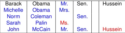
In the politics dataset, most of the mentions con-tain information about people. Therefore, besides canonicalizing named entities, the model also re-solves within-document and cross-document coref-erence, since it assigned a row index for every tion. For example, our model learned that most men-tions ofJohn McCain,Sen. John McCain,Sen. Mc-Cain, andMr. McCainrefer to the same entity. Ta-ble 3 shows a few noteworthy entities from our com-plete model’s output table.
Barack Obama Mr. Sen. Hussein Michelle Obama Mrs.
Norm Coleman Sen. Sarah Palin Ms.
John McCain Mr. Sen. Hussein
Table 3: A small segment of the output table for the poli-tics dataset, showing a few noteworthy correct (blue) and incorrect (red) examples. Black indicates seeds. Though Ms. is technically correct, there is variation in prefer-ences and conventions. Our data include eight instances of Ms. Palin and none of Mrs. Palin or Mrs. Sarah Palin.
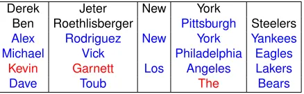
[image:7.612.321.529.396.452.2]Derek Jeter New York
Ben Roethlisberger Pittsburgh Steelers Alex Rodriguez New York Yankees Michael Vick Philadelphia Eagles
Kevin Garnett Los Angeles Lakers
[image:8.612.79.298.60.128.2]Dave Toub The Bears
Table 4: A small segment of the output table for the sports dataset, showing a few noteworthy correct (blue) and in-correct (red) examples. Black indicates seed examples.
introduction of a notion of noise.
In the sports dataset, persons and organizations are mentioned. Recall that success here consists of identifying the correct team for every player. The EEA model is not designed for this and performed poorly. Our model can do better, since it makes use of context information and features, and it can put a person and an organization in one row even though they do not share common words. Table 4 shows a few noteworthy entities from our complete model’s output.
Surprisingly, the model failed to infer thatDerek Jeter plays for New York Yankees, although men-tions of the organizationNew York Yankeescan be found in our dataset. This is because the model did not see enough evidence to put them in the same row. However, it successfully inferred the missing infor-mation forBen Roethlisberger. The next two rows show cases where our model successfully matched players with their teams and put each word token to its respective column. The most frequent error, by far, is illustrated in the fifth row, where a player is matched with a wrong team.Kevin Garnettplays for theBoston Celtics, not theLos Angeles Lakers. It shows that in some cases context information is not adequate, and a possible improvement might be ob-tained by providing more context to the model. The sixth row is interesting becauseDave Toubis indeed affiliated with theChicago Bears. However, when the model saw a mention tokenThe Bears, it did not have any other columns to put the word tokenThe, and decided to put it in the fourth column although it is not a location. If we added more columns, deter-miners could become another attribute of the entities that might go into one of these new columns.
5 Related Work
There has been work that attempts to fill predefined templates using Bayesian nonparametrics (Haghighi and Klein, 2010) and automatically learns template structures using agglomerative clustering (Cham-bers and Jurafsky, 2011). Charniak (2001) and El-sner et al. (2009) focused specifically on names and discovering their structure, which is a part of the problem we consider here. More similar to our work, Eisenstein et al. (2011) introduced a non-parametric Bayesian approach to extract structured databases of entities. A fundamental difference of our approach from any of the previous work is it maximizes conditional likelihood and thus allows beneficial incorporation of arbitrary features.
Our model is focused on the problem of canoni-calizing mention strings into their parts, though itsr variables (which map mentions to rows) could be in-terpreted as (within-document and cross-document) coreference resolution, which has been tackled us-ing a range of probabilistic models (Li et al., 2004; Haghighi and Klein, 2007; Poon and Domingos, 2008; Singh et al., 2011). We have not evaluated it as such, believing that further work should be done to integrate appropriate linguistic cues before such an application.
6 Conclusions
We presented an improved probabilistic model for canonicalizing named entities into a table. We showed that the model adapts to different tasks de-pending on its input and seeds, and that it improves over state-of-the-art performance on two corpora.
Acknowledgements
References
G. Andrew and J. Gao. 2007. Scalable training of L1-regularized log-linear models. InProc. of ICML. N. Chambers and D. Jurafsky. 2011. Template-based
information extraction without the templates. InProc. of ACL-HLT.
E. Charniak. 2001. Unsupervised learning of name structure from coreference data. InProc. of NAACL. J. Eisenstein and E. P. Xing. 2010. The CMU 2008
po-litical blog corpus. Technical report, Carnegie Mellon University.
J. Eisenstein, T. Yano, W. W. Cohen, N. A. Smith, and E. P. Xing. 2011. Structured databases of named entities from Bayesian nonparametrics. In Proc. of EMNLP Workshop on Unsupervised Learning in NLP. M. Elsner, E. Charniak, and M. Johnson. 2009. Struc-tured generative models for unsupervised named-entity clustering. InProc. of NAACL-HLT.
J. R. Finkel, T. Grenager, and C. Manning. 2005. In-corporating non-local information into information ex-traction systems by Gibbs sampling. InProc. of ACL. A. Haghighi and D. Klein. 2007. Unsupervised
coref-erence resolution in a nonparametric Bayesian model. InProc. of ACL.
A. Haghighi and D. Klein. 2010. An entity-level ap-proach to information extraction. In Proc. of ACL Short Papers.
C. S. Jensen, U. Kjaerulff, and A. Kong. 1995. Blocking Gibbs sampling in very large probabilistic expert sys-tem.International Journal of Human-Computer Stud-ies, 42(6):647–666.
R. Jonker and A. Volgenant. 1987. A shortest augment-ing path algorithm for dense and sparse linear assign-ment problems.Computing, 38(4):325–340.
X. Li, P. Morie, and D. Roth. 2004. Identification and tracing of ambiguous names: discriminative and gen-erative approaches. InProc. of AAAI.
D. C. Liu and J. Nocedal. 1989. On the limited memory BFGS method for large scale optimization. Mathemat-ical Programming B, 45(3):503–528.
D. Mochihashi, T. Yamada, and N. Ueda. 2009. Bayesian unsupervised word segmentation with nested Pitman-Yor language modeling. In Proc. of ACL-IJCNLP.
C. Morris. 1983. Parametric empirical Bayes inference: Theory and applications.Journal of the American Sta-tistical Association, 78(381):47–65.
H. Poon and P. Domingos. 2008. Joint unsupervised coreference resolution with Markov logic. InProc. of EMNLP.
S. Singh, A. Subramanya, F. Pereira, and A. McCallum. 2011. Large-scale cross-document coreference using
distributed inference and hierarchical models. InProc. of ACL-HLT.
N. A. Smith and J. Eisner. 2005. Contrastive estimation: training log-linear models on unlabeled data. InProc. of ACL.
R. Tibshirani. 1996. Regression shrinkage and selection via the lasso. Journal of Royal Statistical Society B, 58(1):267–288.