Asymmetry cointegration and the J curve: New evidence from Korean bilateral trade balance models with her 14 partners

Munich Personal RePEc Archive

Asymmetry cointegration and the

J-curve: New evidence from Korean

bilateral trade balance models with her

14 partners

Bahmani-Oskooee, Mohsen and Baek, Jungho

University of Wisconsin-Milwaukee, University of Alaska-Fairbanks

13 February 2016

Online at

https://mpra.ub.uni-muenchen.de/83195/

Asymmetry Cointegration and the J-Curve: New Evidence from Korean

Bilateral Trade Balance Models with her 14 Partners

Mohsen Bahmani-Oskooee

The Center for Research on International Economics The Department of Economics

University of Wisconsin-Milwaukee Milwaukee, WI 53201

bahmani@uwm.edu

and

Jungho Baek Department of Economics

School of Management University of Alaska Fairbanks

jbaek3@alaska.edu

Abstract

Introduction of new econometric methods raises interest in assessing the old theories and the J-curve phenomenon is no exception. Like previous research we first use the linear ARDL approach of Pesaran et al. (2001) to investigate the phenomenon between Korea and each of her 14 trading partners. We then employ recent nonlinear ARDL approach of Shin et al. (2014) to show that in most cases, exchange rate changes have short-run and long-run asymmetric effects on the bilateral trade balances. Separating depreciations from appreciations which is the main feature of the nonlinear model relies upon nonlinear adjustment of the exchange rate and provides relatively more support for the J-curve effect.

.

JEL Classification: F31

I. Introduction

The link between a country’s trade balance and its exchange rate still continues to attract

attention of many researchers. The literature has grown so rapidly that every country now has its own literature and Korea, our country of concern is no exception. Studies that have included Korea in their sample of countries include: Bahmani-Oskooee (1985, 1989), Bahmani-Oskooee and

Malixi (1992), Hsing and Savvides (1996), Lal and Lowinger (2002), Chang (2005), Hsing (2005), and Buyangerel and Kim (2013). These studies have used aggregate trade flows of Korea with the

rest of the world and effective exchange rate of Korean won and have not found strong support for effective depreciation, neither in the short run nor in the long run.1

In order to reduce the aggregation bias, a second group has emerged. Studies in this second

group disaggregate Korean trade flows by trading partners and rely upon bilateral trade data and real bilateral exchange rates. The list includes Wilson (2001), Bahmani-Oskooee and Ratha

(2004a), Bahmani-Oskooee et al. (2005), Sim and Chang (2006), Mustafa and Rahman (2008), Chang (2009), Kim (2009), Bahmani-Oskooee and Harvey (2010), and Wang et al. (2012). The

findings are better than those in the first group but still mixed. These studies have been reviewed in detail by Bahmani-Oskooee et al. (2016) and need no further review here.

The tradition of moving from the first group to the second group was introduced by Rose

and Yellen (1989) who criticized the first group on the ground that they suffer from aggregation bias. To reduce the bias they relied upon a model that was applied to the bilateral trade flows

between the U.S. and each of her six largest trading partners. Using cointegration and error-correction modeling, they then showed that in none of the models the real bilateral exchange rate has short-run nor long-run effects on the bilateral trade balances. Recently, Bahmani-Oskooee and

1

Fariditavana (2016) criticized Rose and Yellen (1989) approach for assuming exchange rate changes to have symmetric effects on the trade balance which necessitate using a linear model.

Once they rely upon a nonlinear ARDL approach of Shin et al. (2014) which is designed to test asymmetric effects of any exogenous variable on the dependent variable, they show that in almost all bilateral trade balance models between the U.S. and each of her six large partners, exchange

rate changes do have significant asymmetric effects on the trade balance in the short run as well as in the long run. As they argue, separating currency depreciations from appreciations seems to

yield significant results that are masked in the linear models that include the real exchange rate as a single entity.

Assessing the asymmetry effects of exchange rate changes and using a nonlinear model

seems to be the direction for current and future research. For example, recently Bussiere (2013) showed that the pass-through of exchange rate changes to import and export prices are asymmetric.

One could then easily argue that if traded goods’ prices respond to exchange rate changes in an asymmetric manner, so should trade itself and eventually the trade balance. Bahmani-Oskooee and

Fariditavana (2016) attribute the asymmetric effects to traders’ expectations and therefore their

responses to currency appreciation which could be different from their expectations and responses to appreciation. Of course, adjustment lags such as production and delivery lags of traded goods

could also be different when a currency depreciates as compared to when it appreciates mostly due to the fact that imports and exports originate from different countries which are subject to two

different rules and institutions.2

In this paper, we add to the small literature on the asymmetry effects of exchange rate changes by considering bilateral trade balances of Korea with each of her 14 largest trading

partners. As can be seen from Table 1 in the Appendix, clearly China tops the list with almost 25% of Korean market and the United States has dropped to the second place. To achieve our goal, we

introduce the models and methods in Section II. In Section III we present our empirical results. Finally, while Section IV concludes the paper, data definition and sources are cited in an Appendix.

II. Models and Methods3

Following Bahmani-Oskooee and Fariditavana (2016) we adopt the following

specification:

where TBi = (Mi/Xi) is a measure of bilateral trade balance between Korea and trading partner i

defined as the ratio of Korean imports from partner i, Mi, over Korean exports to partner i, Xi.

Furthermore, in equation (1), while YKOR measures Korean real income or output, Yi measures the

level of income or output in trading partner i. Finally, REX is the real bilateral exchange rate

between Korean won and partner i’s currency defined in a manner that a decline reflects a real

depreciation of won (see the Appendix). Clearly, if a real depreciation of Korean won is to improve Korean bilateral trade balance, an estimate of d should be positive. Although we expect an estimate of b to be positive and that of c to be negative, indeed both could be negative or positive if increased

income is due to an increase in production of import-substitute goods (Bahmani-Oskooee 1986). Equation (1) is clearly a long-run model and advances in new methods show that in order

to obtain better and stable long-run estimates, we should incorporate the short-run dynamic adjustment process. Therefore, we re-write equation (1) in an error-correction format as in equation (2):

3_{This section closely follows Bahmani-Oskooee and Fariditavana (2016).}

) 1 (

t i,

, ,

,

,t _{KOR t it t}

i a b LnY c LnY d Ln REX

) 2 ( 1 , 4 1 , 3 1 , 2 1 , 1 , 0 , 0 , 0 , 1 , t t i t i t KOR t i j t i n j j t j t i n j j t j t KOR n j j t j t i n j j t t i LnREX LnY LnY LnTB LnREX LnY LnY LnTB LnTB                                         









Equation (2) follows Pesaran et al. (2001) who include the linear combination of lagged level variables rather than lagged error term from equation (1). They then demonstrate that one can

apply the F test to establish joint significance of lagged level variables as evidence of cointegration among the variables. Furthermore, they tabulate new critical values for the F test that accounts for

integrating properties of all variables. For cointegration the calculated F statistic must be above the upper bound critical value.4 Once cointegration is established, the long-run coefficient estimates are derived by the estimates of λ2 –λ4normalized on λ1. The short-run effects are inferred

by the estimates of coefficients attached to first-differenced variables. For example, short-run

effects of exchange rate changes are judged by the estimates of π. Indeed, if estimates of π is

negative at lower lags and positive at higher lags, the J-curve concept will be supported in the short

run.5 However, Rose and Yellen (1989) extended the concept of the J-curve to the long run by defining it as short-run deterioration of the trade balance combined with the long-run

improvement.

The main assumption in both equations (1) and (2) is that all variables have symmetric effects on the trade balance. Concentrating on the real exchange rate, this assumption implies that

if 1% depreciation improves the trade balance by, say, x%, 1% appreciation should hurt it by x%.

4

They prove that their upper bound critical values could be also used when we have combination of I(0) and I(1)

variables in a given model. Since most macro variables are either I(0) or I(1), there is no need for pre-unit root testing

under this approach and this is one of the main advantages of this approach.

5

As argued in the introduction this need not be the case. If not, then exchange rate changes could have asymmetric effects. To address asymmetric effects of exchange rate changes,

Bahmani-Oskooee and Fariditavana (2016) decompose exchange rate changes to two new time series variables where one variable represents solely appreciation which we denote it by POS and the other variable represents solely depreciation which is denoted by NEG. This is done by the concept

of partial sum approach as outlined below:

In equation (3) POSt is the partial sum of positive changes of Ln REXtand NEGt is the partial sum

of negative changes of Ln REXt. Following Shin et al. (2014), we then replace LnREXt variable by

POSt and NEGt in equation (2) to arrive at the following specification:

) 4 ( ' ' ' ' ' ' 1 4 1 3 1 , 2 1 , 1 1 , 0 5 0 4 0 , 3 0 2 0 , 1 1 , , t t t t i t KOR t i n j j t j j t n j j j t i n j j n j j t KOR j n j j t i j t i NEG POS LnY LnY LnTB NEG f POS e LnY d LnY c LnTB b a LnTB                                       











Since construction of the two new variables introduces nonlinearity into equation (4), error-correction model in equation (4) is labeled nonlinear ARDL model, whereas equation (2) is labeled

the linear ARDL model. Shin et al. (2014) then demonstrate that Pesaran et al.’s (2001) bound

testing approach and critical values could equally be applied to equation (4) to establish cointegration. Indeed, they argue that the same critical value of the F that is used in the linear

model should be used in the nonlinear model even though the nonlinear model has one more

variable. This is mostly due to dependency between the POS and NEG variables.6 Once equation (4) is estimated we assess four kinds of asymmetry effects of exchange rate changes on the trade

balance. First, short-run adjustment asymmetry is established if number of lags on ΔPOS are different from number of lags on ΔNEG variable. Second, short-run asymmetry effects is established if size or sign of coefficients (i.e., multipliers) obtained for ΔPOS are different from

size or sign of the same multipliers obtained for ΔNEG, at the same lag. Third, short-run impact

or cumulative asymmetry is established if





established if 3 4. While the first two asymmetry effects will be judged by observation, the

last two will be judged by applying the Wald test.7

III. The Results

In this section, we estimate both the linear ARDL model outlined by equation (2) and the

nonlinear model outlined by equation (4) between Korea and each of her 14 trading partners listed in the Appendix. Generally, quarterly data over the period 1989:Q1-2015:Q1 are used to carry out

the empirical estimation. Exceptions are noted in the Appendix again which also provide sources of the data. To account for Asian Financial Crisis of 1998 and Global Financial Crisis of 2008, we also include two dummy variables in each model. In any autoregressive model, a major concern is

the number of lags imposed on each first-differenced variable. More importantly, since we are to

compare the number of lags on ΔPOSand ΔNEG variable, the order cannot be imposed arbitrary.

Following the literature and Bahmani-Oskooee and Fariditavana (2016), we impose a maximum

6

Note that, as argued by Bahmani-Oskooee and Fariditavana (2016), expected sign of normalized coefficient

estimates of POS and NEG variables in equation (4) are the same as that of REX in equation (2).

7

For some other application of partial sum concept see Apergis and Miller (2006) on the effects of U.S. stock market on consumption; Verheyen (2013) on interest rate pass-through mechanism to deposit rates; and for application of the

of eight lags on each first-differenced variable and use Akaike’s Information Criterion (AIC) to select optimum lags in each case.8 We then report the results from each optimum model in Table

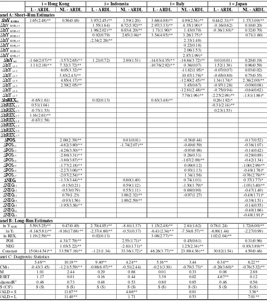
1. In order to follow the table easily, if an estimate (coefficient or statistic) is significant at the 10% level, it is identified by *. Those that are significant at the 5% level, they are identified by **. Critical values are reported at the bottom of Table 1.9

Table 1 goes about here

From the Appendix, we gather that, since China is the largest trading partner of Korea with

almost 24% share of trade, we review the results for Korea-China model first and then summarize for all partners. Estimates of the linear model reveal that in the short-run (Panel A) only levels of economic activities in Korea and China affect the bilateral trade balance. However, the normalized

long-run estimates reported in Panel B reveal that the real bilateral exchange rate carries a significant long-run coefficient. Is this significant coefficient meaningful? The insignificant F

statistic in Panel C indicates that the long-run estimates in this linear model are spurious. To further check for cointegration, we rely upon an alternative test. In this alternative test, we use normalized

long-run estimates and equation (1) and generate the error term, known as error-correction term denoted by ECM. We then replace the linear combination of lagged level variables in the linear ARDL model in equation (2) by ECMt-1 and estimate this new specification after imposing the

same optimum lags. A significantly negative coefficient obtained for ECMt-1 will support

cointegration. Note that the t-ratio that is used to judge significant of this coefficient has a

non-standard distribution for which Banerjee et al. (1989) tabulate critical values for sample sizes such as ours.10 Clearly, the estimate is insignificant again.

8 _{The exception to this rule was the model with China in which the maximum lag order was set at four due to limited}

number of observations.

9

Note that in order to manage the short-run estimates, coefficient estimates of the dependent variable are not reported.

Four additional diagnostic statistics are reported in Panel C. First, to test for first-order autocorrelation, we employ the Lagrange Multiplier (LM) test which has a χ2 distribution with one

degree of freedom. This statistic is insignificant, implying autocorrelation free residuals. Second,

we also report Ramsey’s specification RESET test results. This statistic is also distributed as χ2

with one degree of freedom. This statistic is also insignificant supporting correctly specified

optimum model. Third, to test for stability of short-run and long-run coefficient estimates, we apply CUSUM (denoted by CS) and CUSUMSQ (denoted by CS2) to the residuals of optimum

model. We indicate stable coefficients by “S”and unstable ones by “UNS”. Clearly, all estimates

are stable. Finally, adjusted R2 is reported to reflect the goodness of fit.

To sum up the results from the linear Korea-China model, we conclude that, while level of

economic activities do have short-run effects, none of the three determinants have long-run effects on the bilateral trade balance between the two countries. How does story change if we shift to the

nonlinear model denoted by NL-ARDL. It is now clear that in the short run, levels of economic

activities and won depreciation (ΔNEG) carry significant coefficient. The fact that ΔPOS variable

is insignificant but ΔNEG is significant, supports short-run asymmetric effects of exchange rate

changes. Indeed, this short-run asymmetric effects is further supported by applying the Wald test reported as Wald-S in Panel C. Do short-run effects last into the long run? The answer is in the

affirmative for all variables except Korean income. Furthermore, cointegration is supported by a significant F statistic. Therefore, it appears that introducing nonlinear adjustment of the real

bilateral exchange rate supports cointegration in the nonlinear model which was absent from the linear model. Furthermore, in the long run, while won appreciation has no effect on the bilateral Korea-China trade balance, won depreciation has significantly positive effect. However, this

asymmetric long-run effect is not supported by the Wald test that is reported by Wald-L. Results of other diagnostic statistics are similar to those of the linear model.

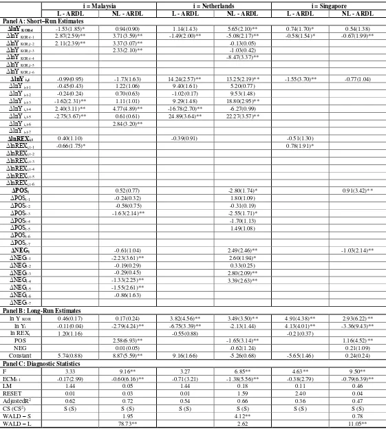
Based on the above analysis, we are now in a position to summarize the results for all models. First, from the short-run estimates we gather that the real bilateral exchange rate carries at least one significant coefficient in the linear model in nine models. In the nonlinear models,

however, either ΔPOS or ΔNEG carry at least one significant coefficient in all models except Korea-United Kingdom model. This supports nonlinear adjustment of the exchange rate which

yield relatively more significant outcomes. Second, short-run adjustment asymmetry is supported in models that belong to Australia, Canada, Germany, Hong Kong, Indonesia, Italy, Malaysia, Netherlands, Thailand, and the U.S. In these 10 models, ΔPOSand ΔNEG take different lag orders.

Third, short-run asymmetric effects are also supported in almost all models, since all short-run estimates obtained for ΔPOS are different in size and sign compared to the estimates obtained for

ΔNEG. However, these short-run asymmetric effects are only significant only in the models of

Korea with China, Hong Kong, Indonesia, Japan, Netherlands, Thailand, and the U.S. due to the

fact that only in these models our Wald-S statistic is significant. Fourth, the bilateral exchange rate caries a significant long-run coefficient in the linear models that belong to China, Hong Kong, Italy, Japan, and Thailand. When we consider the nonlinear models, however, either POS or NEG

carry a significant coefficient in all models except those that belong to Australia, Germany, and the U.K. Again, separating appreciations from depreciations and introducing nonlinear adjustment

of the exchange rate yield more long-run significant results as compared to the linear model. This is further supported by relatively more significant F or ECMt-1 in nonlinear models as compared

Hong Kong, Japan, Malaysia, Singapore, Thailand, and the U.S. Finally, other diagnostic statistics support autocorrelation free residuals, correctly specified optimum models, and stable estimates.

What are the policy implications of our findings? Clearly, separating currency appreciations from depreciations yield insightful results that are masked in the linear models that rely upon the exchange rate itself. For example, in the linear Korea-Canada model, the exchange

rate is insignificant in the long run. If we were to rely upon previous literature and the linear model, we would have concluded that the bilateral exchange rate plays no long-run role in the trade

between Korea and Canada. However, the nonlinear model reveals that, while won depreciation has no long run effects, won appreciation will hurt Korean trade balance with Canada. Exactly opposite is the case in the results with China. While won depreciation will improve Korean trade

balance with China, won appreciation will have no long-run effects. This is also the case with Japan and Italy. Therefore, it appears that the asymmetric effects are partner specific which could

be due to expectations of different trades in different countries. An interesting discovery is that most of the asymmetric effects of exchange rate changes are on the Korean trade with Asian

countries, implying that trades in Asia have different reaction to won depreciation than to won appreciation.

IV. Conclusion and Summary

With advances in econometric literature, old theories are receiving renewed attention and the

J-curve phenomenon in international finance is no exception. The phenomenon basically claims that a devaluation or depreciation worsens the trade balance first and improves it later. When the concept was introduced in the 70s and tested in the 80s, it was considered a short-run phenomenon and

the real exchange rate. Negative coefficients followed by positive ones was said to be a way of supporting the J-curve phenomenon (Bahmani-Oskooee 1985, 1989). However, when

error-correction modeling and cointegration techniques were introduced, Rose and Yellen (1989) argued for a long-run definition, i.e., short-run deterioration combined with long-run improvement. Recently, Bahmani-Oskooee and Fariditavana (2015, 2016) gave us the third definition in which they separate

depreciations from appreciations and define the J-curve to be short-run deterioration combined with long-run improvement only due to depreciation.

Our goal in this paper is to extend the literature on the asymmetric effects of exchange rate changes on the trade balance by considering the experience of Korea. More specifically, we consider bilateral trade balances of Korea with each of her 14 trading partners using quarterly data in order to

test the J-curve phenomenon. Following previous literature, when we first applied the linear ARDL approach of Pesaran et al. (2001), the results provided support for the short-run definition of the

J-curve in the Korean trade balance with Germany, Hong Kong, and Singapore. However, the long-run definition of the J-curve due to Rose and Yellen (1989) received support in the cases of China,

Hong Kong, Italy, Japan, and Thailand. Thus, all in all, using the old tradition and a linear model we find support for the J-curve effect in a total of seven cases. However, when the most recent nonlinear ARDL approach of Shin et al. (2014) was considered, by separating currency depreciations from

appreciations, we find support for the J-curve in the Korean trade balance with China, Hong Kong, Italy, Japan, Thailand and the U.S. We can even add Canada, Indonesia, Malaysia, and Singapore

to the list due to the fact that the variable representing appreciation (i.e., POS) carries a significantly positive coefficient in these models, implying that won appreciation will hurt Korean trade balances with these countries which is in line with our theoretical expectations from the linear

adjustment of the exchange rate yield more support for a successful exchange rate policy. Such findings are absent from previous literature and should be experimented using data from other

APPENDIX

Data Definition and Source

Data Period: Trading partners are ranked in descending order according to the percentage share

of trade engaged in with Korea (2015).

Rank Countries (% share of trade) Data Period

1 China, P.R.: Mainland (23.61%) 2000:Q1 – 2015:Q1 2 United States (11.82%) 1989:Q1 – 2015:Q1

3 Japan (7.42%) 1989:Q1 – 2015:Q1

4 Hong Kong (3.31%) 1989:Q1 – 2015:Q1 5 Australia (2.83%) 1989:Q1 – 2015:Q1

6 Germany (2.82%) 1994:Q2 – 2015:Q1

7 Singapore (2.38%) 1989:Q1 – 2015:Q1 8 Indonesia (1.74%) 1994:Q2 – 2015:Q1 9 Malaysia (1.70%) 1989:Q1 – 2015:Q1 10 United Kingdom (1.40%) 1989:Q1 – 2015:Q1 11 Thailand (1.16%) 1994:Q2 – 2015:Q1

12 Italy (0.97%) 1994:Q2 – 2015:Q1

13 Canada (0.89%) 1989:Q1 – 2015:Q1

14 Netherlands (0.87%) 1994:Q2 – 2015:Q1

Sources:

a. Korea Trade Statistics of the Korea International Trade Association. b. Economic Statistics System of the Bank of Korea.

c. International Financial Statistics of the IMF.

Variables:

TBi = Trade balance of Korea with trading partner i. It is defined as Korea’s imports from partner i over her exports to partner i (source a).

YKOR= Real GDP of Korea (source c).

Yi = Real GDP of trading partner i (source c).

REXi = The real bilateral exchange rate of the currency of partner i against Korean won. It is

defined as REXi = (PKOR*NEXi/Pi) where NEXi is the nominal exchange rate defined as partner i’s currency against Korean won, PKOR is the price level in Korea (measured by CPI) and Pi is the

REFERENCES

Bahmani-Oskooee, M. 1985, “Devaluation and the J-Curve: Some Evidence from LDCs”, The Review of Economics and Statistics, Vol. 67, pp. 500-504.

Bahmani-Oskooee, Mohsen (1986), “Determinants of International Trade Flows: The Case of Developing Countries,” Journal of Development Economics, 20(1), 107-123.

Bahmani-Oskooee, M. 1989, “Devaluation and the J-Curve: Some Evidence from LDCs:

Errata”, The Review of Economics and Statistics, Vol. 69, pp. 553-554.

Bahmani-Oskooee, M. and M. Malixi, 1992. "More Evidence on the J-Curve from LDCs," Journal of Policy Modeling, Vol. 14, pp. 641-653.

Bahmani-Oskooee, M. and Ratha, A. (2004a) “Dynamics of the U.S. Trade with Developing countries”, Journal of Developing Areas, Vol. 37, pp. 1-11.

Bahmani-Oskooee, M. and Ratha, A. (2004b), “The J-Curve: A Literature Review”, Applied Economics, Vol. 36, pp. 1377-1398.

Bahmani-Oskooee, M. and S. Hegerty (2010), “The J- and S-Curves: A Survey of the Recent

Literature”, Journal of Economic Studies, Vol. 37, pp. 580-596.

Bahmani-Oskooee, M. and Harvey, H. (2010) “The J-Curve: Malaysia versus her Major Trading

Partners”. Applied Economics, 42, pp.1067-1076.

Bahmani-Oskooee, M. and H. Fariditavana (2015), “Nonlinear ARDL Approach, Asymmetric Effects and the J-Curve”, Journal of Economic Studies, Vol. 42, pp. 519-530.

Bahmani-Oskooee, M. and H. Fariditavana (2016), “Nonlinear ARDL Approach and the J-

Curve Phenomenon”, Open Economies Review, Vol. 27, pp. 51-70.

Bahmani-Oskooee, M., Goswami, G.G and Talukdar, B.K. (2005) “The Bilateral J-Curve: Australia versus her 23 Trading Partners”,Australian Economic Papers, 44(2), pp. 110-120.

Bahmani-Oskooee, M., Xu, J. and S. Saha (2016), “Commodity Trade between the U.S. and Korea and the J-curve Effect”, New Zealand Economic Papers, forthcoming.

Banerjee, A., J. Dolado, and R. Mestre (1998), “Error-Correction Mechanism Tests in a Single

Equation Framework,” Journal of Time Series Analysis, 19, 267–85.

Bussiere, M. (2013), “Exchange Rate Pass-through to Trade Prices: The Role of Nonlinearities and

Asymmetries”, Oxford Bulletin of Economics and Statistics, 75, 731-758

Buyangerel, B. and Kim, W.J. (2013) “The Effects Of Macroeconomics Shocks on Exchange

Chang, B-K. (2005) “Changes in effects of exchange rate on trade balance according to

Industrial Structural Change”. Journal of Korea Trade, 9(2), pp. 5-23.

De Vita, G. and K. S. Kyaw, (2008), “Determinants of Capital Flows to Developing Countries: A Structural VAR Analysis”, Journal of Economic Studies, Vol. 35, pp. 304-322.

Hajilee, Massomeh, and Omar M. Al-Nasser, (2014), “Exchange Rate Volatility and Stock Market

Development in Emerging Economies”, Journal of Post Keynesian Economics, Vol. 37, pp. 163-180.

Halicioglu, F., (2007), “The J-Curve Dynamics of Turkish Bilateral Trade: A Cointegration

Approach”, Journal of Economic Studies, Vol. 34, pp. 103-119.

Hsing, Han-Min, 2005. “Re-Examination of J-Curve Effect for Japan, Korea and Taiwan”, Japan and the World Economy, Vol. 17, pp. 43-58.

Hsing, H-M., and Andreas Savvides, 1996. “Does a J-Curve Exist for Korea and Taiwan?”, Open Economies Review, Vol. 7, pp. 127-145.

Kim, A. (2009) “An Empirical Analysis of Korea’s Trade Imbalances with the US and Japan”. Journal of the Asia Pacific Economy, 14(3), pp. 211-226.

Lal, A. K. and Lowinger, T.C. (2002), “The J-Curve: Evidence from East Asia”, Journal of Economic Integration, Vol. 17, pp. 397-415.

Magee, Stephen P., (1973), "Currency Contracts, Pass Through and Devaluation," Brooking Papers on Economic Activity, No 1, pp. 303-325.

Mustafa, M. and Rahman, M. (2008) “U.S. Bilateral Nominal Trade Balance with India, Japan,

Malaysia, S. Korea and Thailand, and Bilateral Nominal Exchange Rate Dynamics: Evidence on J-Curve?”Southwestern Economic Review, 35, pp. 153-161.

Pesaran, M. H., Y. Shin, and Smith, R. J. (2001), “Bounds Testing Approaches to the Analysis of Level Relationships,” Journal of Applied Econometrics, Vol. 16, pp. 289-326.

Rose, A.K., and J.L., Yellen (1989), Is There a J-Curve? Journal of Monetary Economics, 24(1), 53-68.

Shin, Y, B. C. Yu, and M. Greenwood-Nimmo (2014) “Modelling Asymmetric Cointegration

and Dynamic Multipliers in a Nonlinear ARDL Framework” Festschrift in Honor of Peter

Schmidt: Econometric Methods and Applications, eds. by R. Sickels and W. Horrace: Springer, 281-314.

Sim, S-H. and Chang, B-K. (2006) “Bilateral Trade Balance between Korea and her Trading Partners: The J-Curve effect”. Journal of Korea Trade, 10(3), pp. 73-93.

Exchange Rate Changes on Trade Balance: Evidence from China and its Trading

Partners”. Japan and the World Economy, 24, pp. 266-273.

Wilson, Peter. (2001) “Exchange Rates and the Trade Balance for Dynamic Asian Economies Does the J-Curve Exist for Singapore, Malaysia and Korea?”, Open Economies Review, Vol. 12, pp. 389-413.

Verheyen, F. (2013) “Interest Rate Pass-Through in the EMU: New Evidence Using Nonlinear

ARDL Framework” Economics Bulletin, 33, 729-739.

Table 1: Full-Information Estimates of Both Linear ARDL (L-ARDL) and Nonlinear ARDL (NL-ARDL) Models (notes at the end) i = Australia i = Canada i = China, Mainland i = Germany L - ARDL NL - ARDL L - ARDL NL - ARDL L - ARDL NL - ARDL L - ARDL NL - ARDL Panel A: Short–Run Estimates

ΔlnY KOR,t 4.04(2.84)** 3.51(2.34)** 0.52(1.21) 1.47(2.70)** -1.41(1.16) 0.28(0.23) 0.11(0.19) 1.33(1.76)*

ΔlnY KOR,t-1 5.38(3.74)** 5.15(3.48)** -2.51(3.65)** 1.90(2.57)** 2.57(3.39)** -0.65(0.98) 3.13(4.11)**

ΔlnY KOR,t-2 1.03(0.86) 0.39(0.31) -1.80(3.66)** -1.60(3.09)**

ΔlnY KOR,t-3 2.89(2.64)** 2.39(2.00)**

ΔlnY KOR,t-4 0.47(0.41) 0.80(0.69)

ΔlnY KOR,t-5 -0.42(0.36) -0.97(0.78)

ΔlnY KOR,t-6 3.22(2.69)** 2.98(2.32)**

ΔlnY KOR,t-7

ΔlnY i,t 4.87(1.35) 6.71(1.77)* -0.06(0.02) 0.53(0.12) 0.46(1.65) 0.21(0.75) 1.64(1.39) 0.84(0.61)

ΔlnY i,t-1 -5.12(1.56) -3.91(0.98) -9.95(2.38)** -0.24(0.05) -0.62(2.25)** -0.69(2.43)**

ΔlnY i,t-2 5.50(1.78)* 6.01(1.75)* 4.02(0.82)

ΔlnY i,t-3 6.24(1.26)

ΔlnY i,t-4 -0.38(0.07)

ΔlnY i,t-5 8.17(1.55)

ΔlnY i,t-6 2.11(0.41)

ΔlnY i,t-7 7.02(1.75)*

ΔlnREXi,t -0.89(2.15)** 1.21(2.62)** -0.26(0.90) -0.67(1.65)

ΔlnREXi,t-1 0.27(0.58) 0.45(1.47) -0.51(1.21)

ΔlnREXi,t-2 1.05(2.15)** 1.08(2.65)**

ΔlnREXi,t-3 0.51(1.23)

ΔlnREXi,t-4 ΔlnREXi,t-5 ΔlnREXi,t-6 ΔlnREXi,t-7

ΔPOSt 0.59(0.79) 1.32(1.42) 0.83(1.54) 1.38(1.63)

ΔPOSt-1 -2.03(2.59)** -0.58(0.52) -2.36(2.52)**

ΔPOSt-2 2.36(2.18)** -0.86(0.90)

ΔPOSt-3 0.22(0.87) -0.43(0.54)

ΔPOSt-4 -0.95(1.14)

ΔPOSt-5 0.70(0.94)

ΔPOSt-6 -1.66(2.30)**

ΔPOSt-7

ΔNEGt -0.35(1.17) 0.22(0.87) -0.98(2.33)** -1.96(3.21)**

ΔNEGt-1 -1.31(1.58)

ΔNEGt-2 1.16(1.57)

ΔNEGt-3 1.17(1.72)*

ΔNEGt-4 0.55(0.84)

ΔNEGt-5 -1.23(2.11)**

ΔNEGt-6 ΔNEGt-7

Panel B: Long-Run Estimates

ln Y KOR -0.93(0.27) 1.01(0.28) 3.55(2.89)** 6.90(7.37)** -4.51(1.63) -3.54(1.38) 3.54(1.22) -15.16(1.50)

ln Yi 1.60(0.29) -5.29(0.67) -6.91(2.94)** -18.02(8.09)** 1.77(1.56) 2.14(1.94)* -11.03(1.08) 4.58(0.60)

ln REXi -0.45(0.63) 0.79(1.29) 0.72(2.02)** -0.73(0.39)

POS 0.46(0.33) 2.38(2.40)** -0.04(0.06) 9.46(1.52)

NEG -1.30(1.07) 0.28(0.87) 0.98(2.56)** -1.39(0.61)

Constant -6.09(0.72) 17.08(0.78) 21.21(3.97)** 48.86(5.87) 15.75(1.75)* 7.54(0.99) 29.17(0.71) 35.86(0.86)

Panel C: Diagnostic Statistics

F 2.38 2.13 3.73 10.16** 3.73 4.59** 1.30 5.98**

ECMt-1 -0.29(1.97) -0.27(1.84) -0.37(3.71)* -0.79(7.01)** -0.42(3.08) -0.45(3.47) -0.15(1.51) -0.18(1.51)

LM 0.38 2.16 0.21 0.46 0.12 0.01 0.05 3.60

RESET 3.11 1.25 0.15 1.39 1.54 0.81 0.20 1.38

AdjustedR2 _{0.55 0.56 0.29 0.38 0.35 0.75 0.44 0.63}

CS (CS2_{) S (S) S (S) S (S) S (S) S (S) S (S) S (S) S (S)}

WALD – S 0.16 0.07 5.42** 0.30

Table 1 continued.

i = Hong Kong i = Indonesia i = Italy i = Japan

L - ARDL NL - ARDL L - ARDL NL - ARDL L - ARDL NL - ARDL L - ARDL NL - ARDL Panel A: Short–Run Estimates

ΔlnY KOR,t 1.65(2.48)** 0.56(0.48) 3.97(2.45)** 1.59(1.20) 3.68(4.08)** 4.99(2.54)** 0.44(2.31)** 1.37(3.09)**

ΔlnY KOR,t-1 1.55(1.64) 6.72(3.92)** 2.97(3.33)** 4.35(1.90)* -0.16(0.62) 0.10(0.20)

ΔlnY KOR,t-2 1.96(2.02)** 6.03(4.20)** 1.71(1.90)* 1.43(0.70) -0.36(1.88)* 0.32(0.70)

ΔlnY KOR,t-3 0.92(0.79) 2.65(1.94)* 3.54(4.05)** 3.26(1.75)* 0.71(1.60)

ΔlnY KOR,t-4 -2.34(2.26)** 2.33(1.48)

ΔlnY KOR,t-5 0.22(0.18)

ΔlnY KOR,t-6 2.06(1.53)

ΔlnY KOR,t-7 2.87(1.99)*

ΔlnY i,t -1.64(2.07)** -3.57(2.65)** 1.21(0.72) 2.80(1.51) -14.03(4.35)** -16.84(3.72)** 0.01(0.01) 0.20(0.19)

ΔlnY i,t-1 1.11(2.18)** 7.32(3.72)** -10.76(2.92)** 0.36(0.07) 1.52(1.38) 0.96(0.59)

ΔlnY i,t-2 6.05(3.32)** -11.82(1.95)* -0.07(0.07) 0.03(0.02)

ΔlnY i,t-3 3.83(2.43)** 10.67(1.76)* -0.65(0.80) 0.75(0.55)

ΔlnY i,t-4 4.85(4.17)** -12.80(2.45)** 1.34(1.74)* 2.36(2.00)**

ΔlnY i,t-5 2.39(2.05)** 3.45(0.67) -0.97(1.26) -0.09(0.08)

ΔlnY i,t-6 -12.81(2.48)** -0.75(0.94) -0.64(0.62)

ΔlnY i,t-7 7.76(1.96)** -2.25(2.98)** -1.81(1.86)*

ΔlnREXi,t -0.65(1.61) 0.02(0.13) 0.63(3.48)** 0.26(1.92)*

ΔlnREXi,t-1 0.51(1.04) -0.31(2.14)**

ΔlnREXi,t-2 -0.73(1.53) 0.23(1.53)

ΔlnREXi,t-3 1.16(2.61)**

ΔlnREXi,t-4 -0.67(1.58)

ΔlnREXi,t-5 ΔlnREXi,t-6 ΔlnREXi,t-7

ΔPOSt 2.00(2.39)** 0.01(0.01) -0.38(0.44) -0.17(0.52)

ΔPOSt-1 -4.62(3.80)** -1.74(2.07)** -0.49(0.59) -0.36(1.07)

ΔPOSt-2 -4.26(3.30)** -0.93(0.98) -0.14(0.42)

ΔPOSt-3 -2.80(3.31)** 0.26(0.31) -0.29(0.89)

ΔPOSt-4 -3.80(3.87)** -1.67(2.09)** -0.42(1.34)

ΔPOSt-5 -1.77(2.18)** 0.09(0.12) -1.00(2.99)**

ΔPOSt-6 -2.27(3.06)** 0.93(1.13) -0.49(1.76)*

ΔPOSt-7 -2.07(2.54)** 1.34(1.56) -0.76(2.79)**

ΔNEGt -1.33(3.44)** 0.60(1.40) 0.74(1.01) 0.37(1.77)*

ΔNEGt-1 -0.15(0.21) 0.59(1.12) -1.30(1.79)* -1.03(3.40)**

ΔNEGt-2 -0.53(0.79) 0.55(1.11) 0.69(0.90) -0.47(1.40)

ΔNEGt-3 0.79(1.23) 1.08(2.32)** -0.97(1.27) -0.49(1.71)*

ΔNEGt-4 -0.93(1.56) 1.00(2.59)** -0.39(1.51)

ΔNEGt-5 -1.95(3.36)** -0.14(0.55)

ΔNEGt-6 -0.40(1.66)

ΔNEGt-7 -0.48(1.91)*

Panel B: Long-Run Estimates

ln Y KOR 5.59(5.25)** 0.47(0.49) 2.70(4.05)** -8.61(1.37) 1.15(2.48)** 2.61(1.62) 0.78(1.24) 1.72(6.00)**

ln Yi -8.14(5.81)** -9.16(17.68)** -2.37(4.60)** -0.51(0.37) -6.41(2.34)** -7.54(6.57)** -6.80(1.44) -2.27(0.99)

ln REXi 1.19(2.59)** 0.02(0.13) 3.08(2.77)** 1.02(2.04)**

POS 4.31(7.79)** 2.55(1.71)* 0.45(0.61) 0.31(0.96)

NEG 1.03(5.22)** -2.61(1.71)* 1.25(2.34)** 0.93(3.89)**

Constant 15.04(4.54)** 33.59(7.16)** -1.21(1.34) 33.36(1.72)* 46.26(3.77)** 23.89(4.36)** 30.82(1.54) 4.50(0.46)

Panel C: Diagnostic Statistics

F 5.48** 10.19** 9.40** 4.24** 5.16** 3.44 6.34** 6.22**

ECMt-1 -0.43(3.45) -1.21(5.59)** -0.88(6.07)** -0.51(2.44) -0.21(3.30) -0.79(3.73)* -0.26(3.60)* -0.76(5.32)**

LM 1.01 2.44 0.29 0.68 0.01 0.33 0.08 2.88

RESET 1.17 0.01 0.16 0.44 3.39 0.02 4.67** 0.12

AdjustedR2 _{0.46 0.73 0.48 0.53 0.80 0.85 0.46 0.56}

CS (CS2_{) S (S) S (S) S (S) S (S) S (S) S (S) S (S) S (S)}

WALD – S 11.67** 4.66** 0.01 3.36*

Table 1 continued.

i = Malaysia i = Netherlands i = Singapore

L - ARDL NL - ARDL L - ARDL NL - ARDL L - ARDL NL - ARDL Panel A: Short–Run Estimates

ΔlnY KOR,t -1.53(1.85)* 0.94(0.90) 1.14(1.43) 5.65(2.10)** 0.74(1.70)* 0.54(1.38)

ΔlnY KOR,t-1 2.87(2.59)** 3.71(3.59)** -1.49(2.00)** -5.08(2.17)** -0.58(1.54)* -0.67(1.99)**

ΔlnY KOR,t-2 2.11(2.39)** 3.37(3.07)** -0.13(0.05)

ΔlnY KOR,t-3 2.33(2.10)** -1.03(0.42)

ΔlnY KOR,t-4 -8.47(3.37)**

ΔlnY KOR,t-5

ΔlnY KOR,t-6

ΔlnY i,t -0.99(0.95) -1.73(1.63) 14.24(2.57)** 13.25(2.19)** -1.55(3.70)** -0.77(1.04)

ΔlnY i,t-1 -0.45(0.43) 1.22(1.06) 9.40(1.61) 5.20(0.77)

ΔlnY i,t-2 -0.24(0.24) 0.70(0.63) -1.02(0.17) 9.53(1.48)

ΔlnY i,t-3 -1.62(2.31)** 1.11(1.01) 9.29(1.48) 18.80(2.95)**

ΔlnY i,t-4 2.40(3.11)** 4.77(4.89)** -16.78(2.70)** -6.27(0.99)

ΔlnY i,t-5 -2.75(3.67)** 0.61(0.61) 24.89(3.64)** 22.27(3.57)**

ΔlnY i,t-6 2.84(3.20)**

ΔlnY i,t-7

ΔlnREXi,t 0.40(1.10) -0.39(0.91) -0.51(1.30)

ΔlnREXi,t-1 -0.66(1.75)* 0.78(1.91)*

ΔlnREXi,t-2

ΔlnREXi,t-3

ΔlnREXi,t-4

ΔlnREXi,t-5

ΔlnREXi,t-6

ΔPOSt 0.52(0.77) -2.80(1.74)* 0.91(3.42)**

ΔPOSt-1 -0.24(0.32) 1.80(1.09)

ΔPOSt-2 -0.58(0.75) -0.31(0.19)

ΔPOSt-3 -1.63(2.14)** -2.55(1.71)*

ΔPOSt-4 -1.70(1.13)

ΔPOSt-5 1.49(1.08)

ΔPOSt-6

ΔPOSt-7

ΔNEGt -0.61(1.04) 2.49(2.46)** -1.03(2.14)**

ΔNEGt-1 -2.23(3.61)** 2.60(1.94)*

ΔNEGt-2 -0.19(0.29) 0.33(0.25)

ΔNEGt-3 -0.29(0.45) 2.80(2.09)**

ΔNEGt-4 -1.33(2.25)** 3.39(2.63)**

ΔNEGt-5 -1.55(2.61)**

ΔNEGt-6 -0.86(1.63)

ΔNEGt-7

Panel B: Long-Run Estimates

ln Y KOR 0.46(0.17) 0.17(0.24) 3.82(4.56)** 3.49(3.50)** 4.91(4.38)** 2.93(6.22)**

ln Yi -0.11(0.04) -2.79(4.24)** -6.75(3.39)** -2.13(1.44) 4.13(4.01)** -3.36(9.43)**

ln REXi 1.20(1.16) -0.55(0.88) -0.21(0.37)

POS 2.58(6.93)** -1.65(3.14)** 1.16(4.52)**

NEG 0.01(0.05) -0.62(1.24) 0.21(1.09)

Constant 5.74(0.88) 8.87(5.59)** 9.16(1.66) -5.26(0.68) -5.65(1.46) 0.24(0.24)

Panel C: Diagnostic Statistics

F 3.33 9.16** 3.27 6.85** 4.63** 9.50**

ECMt-1 -0.17(2.99) -0.60(6.16)** -0.71(3.21) -1.38(5.56)** -0.38(2.79) -0.79(6.39)**

LM 1.44 0.05 1.44 0.18 0.11 0.46

RESET 0.01 0.03 0.01 1.59 2.40 0.04

AdjustedR2 _{0.62 0.72 0.54 0.66 0.36 0.47}

CS (CS2_{) S (S) S (S) S (S) S (S) S (S) S (S)}

WALD – S 1.95 4.12** 0.78

Table 1 continued.

i = Thailand i = United Kingdom i = United States of America L - ARDL NL - ARDL L - ARDL NL - ARDL L - ARDL NL - ARDL Panel A: Short–Run Estimates

ΔlnY KOR,t 0.86(4.46)** 0.85(0.74) 1.49(0.89) -1.12(0.78) 1.02(4.93)** 1.62(1.98)*

ΔlnY KOR,t-1 -2.12(1.83)* 0.05(0.03) -3.65(2.80)** -2.49(2.97)**

ΔlnY KOR,t-2 -0.64(0.76) -1.15(0.76) -3.61(2.94)** -0.59(0.70)

ΔlnY KOR,t-3 0.10(0.14) -2.13(1.54) -3.21(2.67)** -0.14(0.18)

ΔlnY KOR,t-4 2.56(2.62)** -1.22(0.99) -2.54(2.13)** 0.64(0.79)

ΔlnY KOR,t-5 0.60(0.44) 2.55(3.61)**

ΔlnY KOR,t-6 1.77(1.30) 1.21(1.55)

ΔlnY KOR,t-7 3.01(2.22)** 1.14(1.57)

ΔlnY i,t -0.86(4.03)** -0.64(1.22) -2.26(2.20)** -7.24(1.30) -2.26(1.16) -2.24(1.18)

ΔlnY i,t-1 3.87(3.83)** 1.40(0.22) -3.92(2.18)** -2.56(1.35)

ΔlnY i,t-2 2.90(3.50)** 12.30(1.98)* 1.99(1.13) 2.66(1.53)

ΔlnY i,t-3 0.82(1.33) 3.05(0.46) -1.83(0.99) -0.45(0.26)

ΔlnY i,t-4 -16.14(2.61)** -3.71(2.04)** -3.87(2.32)**

ΔlnY i,t-5 1.19(0.20) 3.46(2.10)** 3.48(2.10)**

ΔlnY i,t-6 15.19(2.96)** 2.52(1.48)

ΔlnY i,t-7

ΔlnREXi,t -0.07(0.26) 0.30(1.17) 0.39(1.94)*

ΔlnREXi,t-1 0.14(0.59)

ΔlnREXi,t-2 0.26(1.01)

ΔlnREXi,t-3 0.61(2.30)**

ΔlnREXi,t-4 0.61(2.76)**

ΔlnREXi,t-5 -0.04(0.20)

ΔlnREXi,t-6 0.41(2.11)**

ΔlnREXi,t-7 -0.38(2.11)**

ΔPOSt 1.79(3.41)** 0.47(1.09) 0.34(0.65)

ΔPOSt-1 1.57(2.31)** -1.41(2.71)**

ΔPOSt-2 2.56(3.48)** -0.22(0.42)

ΔPOSt-3 1.40(1.79)* 0.98(1.85)*

ΔPOSt-4 1.42(1.90)* 0.55(1.17)

ΔPOSt-5 1.94(2.76)** 1.08(2.22)**

ΔPOSt-6 0.72(1.38) 1.68(3.73)**

ΔPOSt-7

ΔNEGt -1.16(2.03)** -0.96(1.34) 0.30(1.02)

ΔNEGt-1 -5.25(5.67)** -0.21(0.53)

ΔNEGt-2 -4.75(5.11)** -0.68(1.51)

ΔNEGt-3 -3.46(4.12)** -0.89(1.98)*

ΔNEGt-4 -0.29(0.43) -0.06(0.15)

ΔNEGt-5 -1.27(2.22)** -1.43(3.58)**

ΔNEGt-6 -0.95(2.30)**

ΔNEGt-7 -0.56(1.57)

Panel B: Long-Run Estimates

ln Y IND 1.18(4.78)** 3.59(6.11)** 3.11(2.69)** 3.67(2.16)** 1.75(1.04) 2.45(9.40)**

ln Yi -1.18(4.02)** -2.31(9.48)** -6.30(2.46)** -8.94(2.79)** -4.63(1.33) -3.19(7.09)**

ln REXi 0.72(4.53)** 0.85(1.20) 1.87(1.33)

POS 0.01(0.01) 1.22(1.04) 0.39(3.05)**

NEG 0.91(10.85)** 1.09(1.52) 1.22(9.98)**

Constant 2.14(3.62)** -5.50(3.56)** 21.07(3.20)** 24.50(2.34)** 26.18(1.84)* 4.19(3.55)**

Panel C: Diagnostic Statistics

F 8.88** 8.14** 5.76** 5.04** 4.15* 9.50**

ECMt-1 -0.73(7.54)** -2.18(5.73)** -0.36(4.82)** -0.38(4.43)** -0.12(1.26) -0.90(5.70)**

LM 0.71 2.69 2.24 1.56 0.01 0.44

RESET 0.58 0.04 0.01 0.05 15.62** 11.52**

AdjustedR2 _{0.42 0.69 0.30 0.38 0.62 0.75}

CS (CS2_{) S (S) S (S) S (S) S (S) S (S) S (S)}

WALD – S 22.74** 0.08 17.53**

Notes: a. Numbers inside the parentheses next to coefficient estimates are absolute value of t-ratios. * and ** indicate significance at the 10% and 5% levels, respectively.

b. The upper bound critical values of the F-test for cointegration when there are three (four) exogenous variables are

3.77 (3.52) and 4.35 (4.01) at the 10% and 5% levels of significance, respectively. These come from Pesaran et al.

(2001, Table CI, Case III, p. 300).

c. The critical value for significance of ECMt-1 is -3.47 (-3.82) at the 10% (5%) level when k =3. The comparable

figures when k = 4 are -3.67 and -4.03 respectively. These come from Banerjee et al. (1998, Table 1).

d. LM and RESET are the Lagrange Multiplier statistic to test for autocorrelation and Ramsey’s test for

misspecification, respectively. They are distributed as χ2 _{with one degree of freedom. The critical values are 3.84}