Munich Personal RePEc Archive
On the Gains from Monetary Policy
Commitment under Deep Habits
Givens, Gregory
Department of Economics, Finance and Legal Studies, Culverhouse
College of Commerce, University of Alabama
November 2015
On the Gains from Monetary Policy Commitment under
Deep Habits
Gregory E. Givens
a,*a
Department of Economics, Finance, and Legal Studies, University of Alabama, Tuscaloosa, AL 35487, USA
This Draft: November 2015
Abstract
I study the welfare gains from commitment relative to discretion in the context of an equilibrium model that features deep habits in consumption. Policy simulations reveal that the welfare gains are increasing in the degree of habit formation and economically significant for a range of values consistent with U.S. data. I trace these results to the supply-side effects that deep habits impart on the economy and show that they ultimately weaken the stabilization trade-offs facing a discretionary planner. Most of the inefficiencies from discretion, it turns out, can be avoided by installing commitment regimes that last just two years or less. Extending the commitment horizon further delivers marginal welfare gains that are trivial by comparison.
Keywords: Deep Habits, Optimal Monetary Policy, Commitment, Discretion
JEL Classification: E52, E61
*Corresponding author. Tel.: + 205 348 8961.
1
Introduction
Habit formation has become a fixture of modern equilibrium models of the business cycle. Most take the view that households form habits from consumption of a single aggregate good. That the aggregate good is itself composed of differentiated products, however, raises the question of whether it might be preferable to model consumption habits directly at the level of individual good varieties.
Ravn, Schmitt-Groh´e, and Uribe (2006) adopt this view of preferences, which they de-scribe as “deep habits,” and show that it has two major implications for aggregate dynamics. First, the consumption Euler equation turns out to be identical to the one derived from a traditional habit-persistence model. The essential role that this equation plays in matching certain empirical regularities, notably, consumption and asset-price dynamics, should thus carry over to a deep habits setting as well.1 Second, unlike aggregate-level habits, deep habits
alter firms’ pricing decisions in a way that gives rise to countercyclical mark-ups in equi-librium. Not only is this observation consistent with U.S. experience (e.g., Rotemberg and Woodford, 1999; Mazumder, 2014), recent studies have demonstrated that it also strength-ens the model’s internal propagation mechanisms. Ravnet al. (2006) show that by inducing countercyclical mark-ups, deep habits can account for the observed procyclical responses of consumption and wages to a government spending shock. When grafted into a sticky-price framework, Ravn, Schmitt-Groh´e, Uribe, and Uuskula (2010), Lubik and Teo (2014), and Givens (2015) find that deep habits impart substantial inertia on inflation, thereby lessening the need for dubious features like backward indexation or high levels of exogenous rigidity.2
In light of these and other empirical successes, it is surprising that the literature has had relatively little to say about the normative implications of deep habits. I take up this task here with an application to optimal monetary policy. Specifically, I compute and then ana-lyze the welfare differential between optimal commitment and discretion using a sticky-price equilibrium model that gives prominence to deep habits in consumption. In the context of rational expectations, discretionary policy suffers from a well-known “stabilization bias” (e.g., Woodford, 2003), a dynamic inefficiency that distorts the volatility of the economy’s
1
Standard models of habit formation have been used to resolve the equity premium puzzle (e.g., Abel, 1990; Constantinides, 1990) as well as the risk-free-rate puzzle (e.g., Campbell and Cochrane, 1999). They also appear frequently in medium-scale DSGE models to generate the “hump-shaped” responses of aggregate consumption and output to various economic shocks identified in the data (e.g., Christiano, Eichenbaum, and Evans, 2005; Smets and Wouters, 2007).
2Zubairy (2014b) shows that deep habits provide a transmission channel for government spending shocks
response to unexpected shocks. Policymakers can reverse these distortions and, in the pro-cess, advance the welfare of private agents by switching to optimal commitment. The extent to which commitment increases welfare, however, is plainly model dependent. So in prac-tice, establishing whether the gains are large or small is ultimately an empirical matter. The superior fit displayed by models containing deep habits suggests that they could provide credible information on the potential size of these gains in the real world.
The case for estimating the gains from commitment using only data-consistent models was first made by Dennis and S¨oderstr¨om (2006) who argued that such information is critical in deciding whether public investments in the economy’s commitment technology justify the costs. To provide context, the authors estimated the welfare gap using several famous empir-ical models and found substantial variation among them. Obscuring their results, however, is the fact that the models featured in the study lack coherent microeconomic foundations and, as such, are incapable of providing an ideal measure of social welfare consistent with household preferences. As a result, the authors took the usual step of articulating social welfare through an exogenously-specified loss function defined over the weighted variances of inflation, the output gap, and nominal interest rate smoothing (e.g., Rudebusch and Svens-son, 1999). But without explicit reference to private utility, it is doubtful that such an objective function encapsulates the true welfare cost of discretion.
I avoid this critique here by employing the correct measure of welfare based on a quadratic approximation of the average household’s utility function. As shown by Leith, Moldovan, and Rossi (2012), it is possible to write the approximation as a particular weighted sum of three terms: squares of inflation, the output gap, and the “habit-adjusted” output gap (i.e., deviations from Pareto-efficient levels). To compute the welfare differentials, I maximize this criterion separately under commitment and discretion and record the value function in both cases. Gaps between the two are then converted into units of consumption in order to provide a tangible interpretation of the losses generated by the stabilization bias.
extensions to the model, however, are unnecessary here. As explained by Leithet al. (2012), incorporating deep habits elicits an endogenous policy trade-off between inflation and the two output gap concepts described above. Such a trade-off emerges because the consump-tion externality induced by habit formaconsump-tion drives a wedge between the flexible-price (zero adjustment cost) equilibrium and the efficient equilibrium. Thus any shock to the economy– whether it be a preference or a productivity shock–creates tension between two separate policy goals in the short run: minimizing price adjustment costs and neutralizing the habit externality. The former is achieved by holding inflation equal to target inflation and the latter by aligning output with its efficient level (i.e., a zero output gap).
Policy simulations carried out in this paper confirm that the welfare differential between commitment and discretion is strictly increasing in the degree of deep habits and economi-cally significant for a range of values that span known estimates. At the habit value estimated by Ravn et al. (2006), for example, the gap is equivalent to 0.188 percent of consumption, or about $90 per person per year. Most of the gains from commitment, it turns out, trace directly to the restrictions that deep habits impose on the log-linearized Phillips Curve equa-tion. There one sees that the main forcing process for inflation depends positively on the real interest rate in addition to firms’ marginal cost of production. This means that adjust-ments to the interest rate will have immediate supply-side effects on inflation that counteract the familiar demand-side effects of policy on marginal cost. Such opposing influences will obviously frustrate efforts to stabilize inflation under either policy. Quantitative results show, however, that these adverse supply-side effects, which become stronger as deep habits intensify, are easier to manage with commitment than with discretion.
most of the gains identified in the benchmark analysis are attainable with commitments last-ing no more than two years on average. Further increases in the durability of commitments produces marginal welfare gains that are much smaller by comparison.
2
The Model
Economic activity results from interaction between optimizing households and imperfectly competitive firms that manufacture differentiated products and face costs of changing prices.
2.1
Households
There is a unit measure of households, indexed by j, that gain utility from consuming a composite of differentiated goods xj,t and lose utility from supplying labor hj,t. Following
Ravnet al. (2006), households developexternal consumption habits at the level of individual good varieties. This so-called “deep habits” arrangement assumes that the composite good takes the form
xj,t = [∫ 1
0
(cj,t(i)−bct−1(i))1−1/ηdi
]1/(1−1/η)
, (1)
wherecj,t(i) is consumption of goodiby householdj andct(i)≡∫01cj,t(i)dj is the population
mean consumption of the same item. The parameter η > 1 determines the intratemporal substitution elasticity across (habit-adjusted) varieties, and b ∈[0,1) measures the strength of habit formation. For b >0, preferences feature “catching up with the Joneses” `a la Abel (1990) but on a good-by-good basis. Setting b= 0 removes deep habits from the model, and with it, the consumption externality that creates trade-offs for optimal stabilization policy.
Every period householdj minimizes∫1
0 Pt(i)cj,t(i)disubject to the aggregation constraint
(1). First-order conditions imply demand functions of the form
cj,t(i) = (
Pt(i) Pt
)−η
xj,t+bct−1(i),
wherePt(i) is the price of goodiandPt≡ [
∫1
0 Pt(i)
1−ηdi]1/(1−η)is the price of the composite
good. Note that demand for good idepends on past aggregate salesct−1(i) as long asb >0.
Intertemporal spending decisions are made with reference to a lifetime utility function
Vj,0 =E0
∞
∑
t=0
βtat [
x1j,t−σ
1−σ − h1+j,tχ
1 +χ
]
, (2)
where E0 is a date-0 expectations operator and β ∈ (0,1) is a subjective discount factor.
Parameter σ > 0 governs the intertemporal elasticity of consumption and χ > 0 the Frisch elasticity of labor supply. Preference shocksataffect all households symmetrically and follow
the autoregressive process logat=ρalogat−1 +εa,t, with |ρa|<1 and εa,t∼i.i.d. (0, σ2a).
Households enter each period with riskless one-period bond holdings Bj,t−1 that pay
a gross nominal interest rate Rt−1 at date t. They also provide labor services to firms
at a competitive nominal wage rate Wt and, after production, receive dividends Φj,t from
ownership of those firms. The period-t budget constraint is
Ptxj,t+ϖt+Bj,t ≤Rt−1Bj,t−1+ (1−τ)Wthj,t+ Φj,t+Tj,t, (3)
where ϖt ≡ b∫01Pt(i)ct−1(i)di.3 Sequences {xj,t, hj,t, Bj,t}∞t=0 are chosen to maximize Vj,0
subject to (3) and a no-Ponzi requirement, taking as given{at, Pt, ϖt, Rt−1, Wt,Φj,t, Tj,t}∞t=0
and initial assets Bj,−1. The first-order conditions satisfy
1 =βEt Rt πt+1
at+1
at (
xj,t xj,t+1
)σ
, (4)
hχj,txσj,t =wt(1−τ), (5)
where wt ≡Wt/Pt is the real wage andπt ≡Pt/Pt−1 is the gross inflation rate.
Equation (4) is the Euler equation for (habit-adjusted) consumption, and (5) is an ef-ficiency condition linking the marginal rate of substitution to the real wage. Notice that the tax rate τ ∈[0,1] on labor income drives a wedge between these two quantities. As ex-plained in Leith et al. (2012), taxes are used to fund lump-sum transfers Tj,t to households,
and the value of τ is chosen so that steady-state allocations are Pareto efficient despite the distortionary effects of habit externalities. Such a tax enables one to obtain a valid quadratic approximation of expected utility when evaluated using only a linear approximation of the model’s equilibrium conditions (e.g., Woodford, 2003).
3Householdj’s efforts to minimize the cost of assembling each unit ofx
j,t implies that, at the optimum, ∫1
0 Pt(i)cj,t(i)di=Ptxj,t+b
∫1
2.2
Firms
Good i is produced by a monopolistically competitive firm with technology yt(i) = ztht(i),
whereyt(i) is the output of firmiandht(i) its use of labor. Technology shocksztare common
to all firms and follow logzt=ρzlogzt−1+εz,t, with |ρz|<1 and εz,t∼i.i.d. (0, σz2).
Firms maximize the present value of profit subject to
ct(i) = (
Pt(i) Pt
)−η
xt+bct−1(i), (6)
a market demand curve obtained by integrating cj,t(i) over all j ∈[0,1] households.4 Firms
stand ready to meet demand at the posted price, so ztht(i)≥ct(i) for all t≥ 0. Individual
prices may be reset every period, but at a cost. Following Rotemberg (1982), firms pay adjustment costs of the form (α/2) [Pt(i)/πPt−1(i)−1]2yt, measured in units of aggregate
output yt ≡ ∫1
0 yt(i)di, anytime growth in Pt(i) deviates from the long-run mean inflation
rate π. The constantα ≥0 determines the size of price adjustment costs. The Lagrangian of firm i’s maximization problem is
L= E0
∞
∑
t=0
q0,t {
Pt(i)ct(i)−Wtht(i)− α
2
[
Pt(i) πPt−1(i)
−1
]2
Ptyt
+Ptmct(i) [ztht(i)−ct(i)] +Ptνt(i) [
(
Pt(i) Pt
)−η
xt+bct−1(i)−ct(i) ]}
,
where q0,t is a stochastic discount factor.5 Sequences {ht(i), ct(i), Pt(i)}∞t=0 are chosen to
maximize L, taking as given {q0,t, Wt, Pt, yt, zt, xt}∞t=0 and initial values c−1(i) and P−1(i).
The first-order conditions are
wt=mct(i)zt, (7)
νt(i) = Pt(i)
Pt
−mct(i) +bEt q0,t+1
q0,t
πt+1νt+1(i), (8)
4
xt≡∫
1
0 xj,tdj. 5
In equilibrium the stochastic discount factor satisfiesq0,tPt =βtatx−tσ. It is interpreted as the date-0
ct(i) = ηνt(i) (
Pt(i) Pt
)−η−1
xt+α (
Pt(i) πPt−1(i)
−1
)
Ptyt πPt−1(i)
−αEt q0,t+1
q0,t πt+1
(
Pt+1(i)
πPt(i)
−1
)
Pt+1(i)Ptyt+1
πPt(i)2
. (9)
The multipliermct(i) in (7) corresponds to real marginal cost. The multiplierνt(i) in (8)
is the shadow value of selling an extra unit of good i. It equals the profit generated by the sale of that unit in periodt, Pt(i)/Pt−mct(i), plus all discounted future profit that the sale
is expected to yield via habit formation, bEtq0q,t0,t+1πt+1νt+1(i). Without consumption habits
(b= 0), νt(i) just equals current marginal profit. The third optimality condition (9) equates
the costs and benefits of unit changes to the firm’s relative pricePt(i)/Pt.
2.3
Government
The government has a dual role in the model. First, it taxes labor income and remits the proceeds to households as lump-sum transfers. There is no government spending and no public debt, so τ Wthj,t = Tj,t for all j ∈ [0,1]. Second, it conducts monetary policy by
adjusting the nominal interest rate Rt. Policy outcomes are optimal in that they maximize
(under commitment or discretion) a second order approximation to V0 ≡
∫1
0 Vj,0dj.
2.4
Competitive Equilibrium
In a symmetric equilibrium households make identical spending and labor supply choices and firms charge the same price. It follows that subscriptj and argument ican be dropped from the constraints and optimality conditions.6 Equilibrium also requires imposing relevant
market-clearing conditions. Balancing the supply and demand for labor means ∫1
0 hj,tdj =
∫1
0 ht(i)di≡ ht for t ≥0. In product markets, supply of the final good equals demand from
consumption plus resources spent on adjustment costs, so yt =ct+ (α/2)(πt/π−1)2yt.
2.5
Calibration
Table 1 reports benchmark numerical values for the structural parameters. Most are similar to ones appearing in other studies that build deep consumption habits into sticky-price models of the business cycle (e.g., Leith et al., 2012; Zubairy, 2014a; Lubik and Teo, 2014).
6
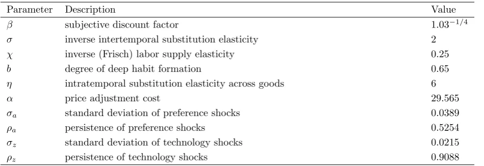
Table 1
Benchmark parameter values
Parameter Description Value
β subjective discount factor 1.03−1/4
σ inverse intertemporal substitution elasticity 2
χ inverse (Frisch) labor supply elasticity 0.25
b degree of deep habit formation 0.65
η intratemporal substitution elasticity across goods 6
α price adjustment cost 29.565
σa standard deviation of preference shocks 0.0389
ρa persistence of preference shocks 0.5254
σz standard deviation of technology shocks 0.0215
ρz persistence of technology shocks 0.9088
The unit of time is one quarter. The discount factor β is set to 1.03−1/4, implying a
steady-state annual real interest rate of 3 percent. Utility parameters, σ and χ, are fixed so that the model delivers an intertemporal elasticity of substitution (1/σ) equal to one-half and a Frisch labor supply elasticity (1/χ) equal to four. Both values are broadly consistent with estimates drawn from medium-scale DSGE models (e.g., Smets and Wouters, 2003; Levin, Onatski, Williams, and Williams, 2006; Justiniano, Primiceri, and Tambalotti, 2010). The habit parameter b is initially set equal to 0.65. While this is a bit smaller than what recent empirical evidence suggests, it is close to the benchmark value in Leith et al. (2012).7
In most of the policy experiments discussed below, I vary b on the interval [0,1) since the goal here is to scrutinize how the gains from commitment are affected by deep habits.
The substitution elasticity η along with β and b jointly determine firms’ steady-state mark-up.8 I set the value of η to 6, implying an average mark-up of 20.33 percent under
the benchmark calibration. However, mark-ups can range from 20 and 23 percent depending on the size of b. As for adjustment costs, I fix α so that the model is consistent with a price-change frequency of 9 months in a Calvo-Yun framework. In the absence of deep habits, the Phillips Curve coefficient on real marginal cost, obtained by log-linearizing (9) around the non-stochastic steady state equilibrium (see section 3.2), is (η−1)/α. Equating this term to its counterpart in a Calvo-Yun Phillips Curve and solving for α gives α =
ϕ(η−1)/(1−ϕ)(1−βϕ), where 1−ϕ is the reset probability. Setting ϕ = 2/3 implies an
7
Estimates ofb found in Ravnet al. (2006), Ravnet al. (2010), and Lubik and Teo (2014) span 0.85 to 0.86. Point estimates obtained by Givens (2015) put the value closer to 0.94.
8
Table 2 Model fit
σ(ˆπt) σ(∆ˆct) σ( ˆRt) ρ(ˆπt,∆ˆct) ρ(ˆπt,Rˆt) ρ(∆ˆct,Rˆt) ρ(ˆπt,πˆt−1) ρ(∆ˆct,∆ˆct−1) ρ( ˆRt,Rˆt−1) Data 0.5028 0.6137 0.8238 −0.1244 0.6456 0.0711 0.6527 0.2839 0.9735 Model 0.5409 0.6042 0.8054 −0.1116 0.6585 0.0685 0.5429 0.3668 0.8428
Notes: Sample is 1980:Q1-2014:Q4. σ(Xt) = variance ofXt;ρ(Xt, Zt) = contemporaneous correlation between Xt and Zt;
ρ(Xt, Xt−1) = first-order autocorrelation ofXt. The sample Taylor rule is ˆRt= 0.6927ˆπt+ 0.4418∆ˆct+ 0.7961 ˆRt−1, and the value of the objective function(ΩY( ˆΨ)−ΩˆY
)′(
ΩY( ˆΨ)−ΩˆY
)
= 0.0382.
average price duration of 3 quarters and is equivalent to α= 29.56 in the present model. To obtain values for the parameters characterizing preference and technology shocks, I use a simplified version of the estimation program outlined in Coibion and Gorodnichenko (2011). In short, values for (ρa, σa, ρz, σz) are chosen to match, as closely as possible,
a small set of contemporaneous and intertemporal covariances of the model’s observable variables with corresponding moments from U.S. data. There are three variables in the deep habits model for which macroeconomic time-series data are available: the growth rate of consumption, the inflation rate, and the nominal interest rate. To compute moments for these variables, I first log-linearize the equilibrium conditions and solve for the unique rational expectations equilibrium (e.g., Klein, 2000). I then extract the relevant moments from the reduced-form representation of the model. This exercise obviously requires making an assumption about monetary policy. Here I assume that interest rates are set according to a Taylor-type rule of the form ˆRt = θππˆt+θc(ˆct−ˆct−1) +θRRˆt−1, which allows policy
to respond to current levels of inflation and consumption growth and lagged levels of the interest rate.9 The policy-rule coefficients, together with the stochastic shocks, are picked to
minimize the discrepancy between select model moments and their sample counterparts. Denote Ψ = (ρa, σa, ρz, σz, θπ, θc, θR) the subset of parameters to be estimated via
method-of-moments and Yt = [ˆπt ∆ˆct Rˆt]′ the vector of observables.10 In estimating Ψ, I focus only
on matching the variances of ˆπt, ∆ˆct, and ˆRt, the contemporaneous correlations between
them, and the first-order autocorrelations for each. The formal estimate of Ψ is
ˆ
Ψ = argmin
Ψ
(
ΩY(Ψ)−ΩˆY )′(
ΩY(Ψ)−ΩˆY )
,
where ΩY(Ψ) are theoretical moments computed for a given Ψ and ˆΩY are the corresponding
9
For any variableXt, ˆXt≡logXt−logX, the log deviation of Xtfrom its steady-state value X.
10
sample moments.11 Holding the rest of the structural parameters fixed at their benchmark
values, estimates of the law of motion for preference shocks areρa = 0.5254 andσa = 0.0389.
Estimates of the technology shock process are ρz = 0.9088 and σz = 0.0215. Both sets are
listed in Table 1. The values of ΩY( ˆΨ) and ˆΩY are reported in Table 2.12
3
Optimal Policy
The central task of this paper is to assess the gains from commitment relative to discretion using a modeling framework that gives prominence to deep consumption habits. The last section described the full model of private behavior and established plausible numerical values for the structural parameters. The next step is to specify the government’s optimization problem so that equilibrium welfare under the two policies can be compared.
3.1
Policy Objectives
The welfare criterion used to quantify the gains from precommitment is given by a second-order Taylor series expansion of households’ expected lifetime utility. As shown by Leith et al. (2012), a quadratic approximation to (2) can be written as
V0 =−
1 2h
1+χE
0
∞
∑
t=0
βt
{
απˆt2+χ(ˆyt−yˆte)2+
σ(1−b)
1−βb (ˆxt−xˆ e t)
2}
+t.i.p.+O(∥ε∥3), (10)
where ∥ε∥ is a bound on the amplitude of preference and technology shocks, O(∥ε∥3) are
terms in the expansion that are of third order or higher, and t.i.p. collects terms that are independent of monetary policy.13 The quantities in (10) that depend on policy include
squares of inflation as well as two different output gap variables, namely, deviations of actual and habit-adjusted output from their Pareto-efficient levels, denotedye
t and xet, respectively.
That both output gap terms appear separately in the policy objective function is a direct consequence of habit formation. As b approaches zero, the two terms fold into a single
11Ω
Y ≡[var(ˆπ)var(∆ˆc)var( ˆR)corr(ˆπ,∆ˆc)corr(ˆπ,Rˆ)corr(∆ˆc,Rˆ)corr(ˆπ,πˆ−1)corr(∆ˆc,∆ˆc−1)corr( ˆR,Rˆ−1)]′. 12The sample covers U.S. data from 1980:Q1 to 2014:Q4. Consumption growth is log(RP CE
t/P OPt)−
log(RP CEt−1/P OPt−1), where RP CE is chained Real Personal Consumption Expenditures (PCE) and
P OP is the Civilian Noninstitutional Population. Inflation equals log(Pt/Pt−1) and is constructed using
the chain-type price index for PCE. The interest rate is log(1 +T Bt/100)1/4, where T B is the secondary
market rate on 3-Month Treasury Bills. All three variables are de-meaned prior estimation. Average annual inflation over the sample is 2.75 percent. I use this value to calibrate steady-state inflation in the model.
13
objective given by (χ+σ) (ˆyt−yˆte)
2
, in the process simplifying (10) to the familiar welfare measure associated with the basic sticky-price model discussed in Woodford (2003).
The fact that inflation and the output gap variables enter the objective function strictly as second-order terms is important because it means that their expected values can be computed from a simple log-linear approximation to the model’s equilibrium conditions. Following Leithet al. (2012), the linear-quadratic nature of the problem is made possible by the use of a taxτ on labor income that renders the steady-state allocations Pareto efficient. Since adjustment costs are zero in the steady state, the tax eliminates only thenet distortions caused by habit externalities and market power. Under the benchmark calibration, this is accomplished with a tax rate of 57.31 percent.14
3.2
Policy Constraints
The government conducts monetary policy by setting ˆRt to maximize the approximate
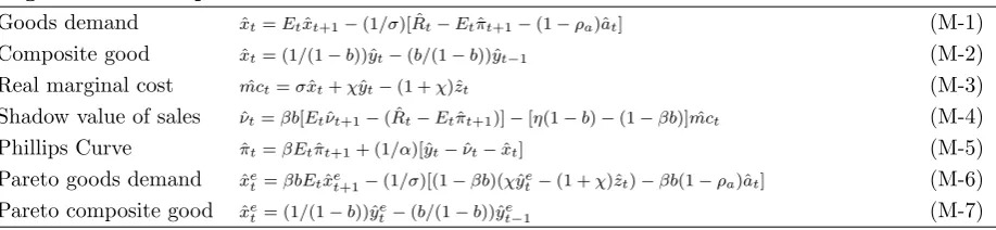
wel-fare criterion described above. The constraints on policy are given by the log-linearized equilibrium conditions of the deep habits model, which for the sake of clarity I present in Table 3. Because the constraints are forward looking, whether the government can credibly commit to a sequence of actions, or whether policy decisions are made independently every period (i.e., discretion), has a big impact on the economy. If commitments are feasible, interest rates evolve according to an optimal state-contingent rule. In designing such a rule, the government internalizes the effect of its own choices on the expected future variables in (M-1)–(M-7). The result is a socially optimal equilibrium in which policy makes effi-cient use of private-sector beliefs to achieve the stabilization goals embodied by (10). By contrast, outcomes under discretion are not the ones prescribed by some fixed contingency rule. Every period a discretionary optimizer resets policy in response to current conditions, taking agents’ beliefs about the future as given. The equilibrium is only optimal in a limited sense because absent commitment the government cannot harness expectations in a way that eases its stabilization trade-offs. This inability to manage expectations is the source of the stabilization bias of discretionary policy discussed earlier. Computational programs used to solve for equilibria under commitment and discretion are taken from S¨oderlind (1999).
14Setting τ = 1−(1/mc)(1−βb) ensures that the decentralized allocations are Pareto-optimal in the
Table 3
Log-linearized deep habits model
Goods demand xˆt=Etxˆt+1−(1/σ)[ ˆRt−Etˆπt+1−(1−ρa)ˆat] (M-1) Composite good xˆt= (1/(1−b))ˆyt−(b/(1−b))ˆyt−1 (M-2)
Real marginal cost mcˆt=σxˆt+χyˆt−(1 +χ)ˆzt (M-3) Shadow value of sales νˆt=βb[Etνˆt+1−( ˆRt−Etˆπt+1)]−[η(1−b)−(1−βb)] ˆmct (M-4) Phillips Curve πˆt=βEtˆπt+1+ (1/α)[ˆyt−ˆνt−xˆt] (M-5) Pareto goods demand xˆe
t=βbEtxˆet+1−(1/σ)[(1−βb)(χyˆte−(1 +χ)ˆzt)−βb(1−ρa)ˆat] (M-6) Pareto composite good xˆe
t= (1/(1−b))ˆyet−(b/(1−b))ˆyet−1 (M-7)
3.3
Welfare Gaps
In the next section I quantify the welfare gap between discretion and commitment. One way to measure the gap is by computing the percentage gain in welfare that accompanies a switch from the former policy to the latter. This quantity is given by 100×(
1−Vc
0/V0d
)
, whereVc
0 andV0dare the maximal values of (10) obtained under commitment and discretion.
The percentage gain metric, however, is hard to interpret because it involves only indirect utility values. I therefore consider a second concept that translates Vc
0 and V0d into units
of consumption. Specifically, I compute the drop in the consumption path associated with commitment needed to balance welfare under the two policies. This quantity, call it λ, is defined by
E[
V0d]
=E ∞
∑
t=0
βtat [
((1−λ)xc t)
1−σ
1−σ −
(hc t)
1+χ
1 +χ
]
, (11)
where{xc
t, hct}∞t=0 are sequences for consumption and work hours under commitment andEis
an unconditional expectations operator.15 The value ofλputs into perspective the magnitude
of the welfare gap between commitment and discretion caused by the stabilization bias.
4
Welfare Analysis
Having discussed the government’s stabilization goals and the procedural differences be-tween commitment and discretion, I can now analyze the extent to which the gains from commitment are affected by deep habits.
15
4.1
Gains from Commitment
The focal point of the analysis is Fig. 1, which plots the welfare differential expressed in units of consumption for values of b ∈ [0,0.94].16 The solid line corresponds to the deep
habits model. Consider first the benchmark calibration. When b = 0.65, the gap between commitment and discretion is equivalent to 0.0247 percent of consumption. Per capita U.S. nominal consumption expenditures was $48,674.47 (annualized) in the last quarter of 2014, so a loss of 0.0247 percent amounts to $12.02 per person per year. In comparison, Leith et al. (2012) estimate the welfare gap to be 0.0047 percent of consumption, or $2.26 per person. The difference here can be traced to the fact that the current model allows for shocks to preferences as well as total factor productivity. Leith’s model contains only the latter. It turns out that both supply and demand-side shocks generate trade-offs for a policymaker faced with stabilizing inflation in addition to the output gap (see section 4.3). Removing one of the shocks lessens the tension between these objectives, in the process narrowing the gap between precommitment and discretionary outcomes.
The results also show that λ varies greatly with the size of the habit parameter. When
b is one-half, the gap between commitment and discretion is equivalent to 0.0073 percent of consumption or $3.58. Lowering b to 0.25 reduces λ to a mere 0.0007 percent.17 Moving in
the opposite direction I find that the value of commitment increases dramatically as habits strengthen. Shifting b from 0.8 to 0.9 raises λ from 0.0915 to 0.3603 percent, that is, from $44.53 to $175.38 per person. The gap balloons to almost $400 whenbnears the upper bound of the parameter space. Given the sensitivity of these findings, locating empirically relevant values for b is critical for obtaining a reliable estimate of λ. Studies that have attempted to estimate the degree of deep habits indicate that the true value is probably close to 0.86 (e.g.,
Ravn et al., 2006; Lubik and Teo, 2014). Evaluated at this point, the benchmark model
produces a welfare gap equivalent to 0.188 percent of consumption, or about $90 per person. It is clear that the welfare gains from commitment can be large, notably for values of b
consistent with the data. But precisely how deep habits enable these gains to emerge is an open question. To shed light on the matter, recall that habit formation, because it affects the intertemporal spending decisions of households as well as the optimal price-setting behavior of firms, imposes separate restrictions on the demand and supply-side components of the structural model. Of course, both sets of restrictions influence the policy trade-offs that
16Optimal discretion does not produce a stable equilibrium in the deep habits model whenb >0.94. 17Whenb = 0 neither preference nor technology shocks create trade-offs for the government. It follows
0 0.1 0.2 0.3 0.4 0.5 0.6 0.7 0.8 0.9 1 −0.1
0 0.1 0.2 0.3 0.4 0.5 0.6 0.7 0.8 0.9 1
b
λ
×
100 (%)
$0.32
$0.12
$3.58
$0.73 $1.68
$12.02
$3.85 $44.53
$7.41 $10.10 $175.38
[image:16.595.116.486.88.350.2]$390.37
Fig. 1. The percent drop in consumption (λ×100) sufficient to equalize welfare under commitment and discretion is shown
for values ofb∈[0,0.94]. The solid line corresponds to the deep habits model and the dashed line the aggregate habits model. Dollar values are found by multiplyingλby $48,674.47, per capita U.S. nominal consumption expenditures in 2014:Q4.
account for the welfare gaps seen in Fig. 1. The basic goal here is to identify which side of the model plays the dominant role in the sudden growth of these gaps as habits intensify.
To sort out the supply-side effects of deep habits from the demand-side effects, I add to the figure the relationship between λ and b derived from a traditional model of habit formation in which consumption externalities originate at the level of composite goods rather than individual good varieties (e.g., Smets and Wouters, 2003). The comparison is informative because the externalities present in this modelin equilibriumare indistinguishable from those of the benchmark model even though the underlying structure of consumption habits is very different.18 In fact, one can show that the two arrangements have identical implications for
aggregate demand. The result is that (M-1)–(M-3) are exactly the same in both models. Where they differ is with regard to aggregate supply. As discussed in Givens (2015), the shadow value of sales described by (M-4) simplifies to ˆνt =−(η−1) ˆmctwhen the composite
18
good is habit-forming but not differentiated goods. Substituting this expression into (M-5) produces the canonical New Keynesian Phillips Curve, ˆπt=βEtπˆt+1+ ((η−1)/α) ˆmct, that
links inflation to current and expected future marginal cost (e.g., Gal´ı and Gertler, 1999). All other aspects of the model, including the policy objective function, are equivalent to the benchmark deep habits specification.19 It follows that any discrepancy in the value of λ
across models should be attributed solely to the supply-side effects of deep habits.
The dashed line shows the welfare differential for the comparison model, referred to in the figure as the “aggregate habits” model. Here estimates of λ are uniformly smaller and far less sensitive to changes in the habit parameter. Forb= 0.65, the gap between discretion and commitment is worth 0.0034 percent of consumption, or $1.68 per person. Increasing
b all the way to 0.94 raises λ to just 0.0208 percent, or $10.10 per person. At this point, the value of λ implied by the deep habits model exceeds that of the aggregate habits model by an amount equal to $380.27. Thus one can conclude that the gains from commitment seen in the benchmark analysis, particularly for large values of b, are principally the result of the supply-side influences that deep habits impart on the economy. The gains attributed to demand-side effects per se appear modest by comparison.
4.2
Volatilities
Although welfare analysis points to sizable gains from commitment in the deep habits model, it is not yet clear how these gains manifest in terms of the volatilities of the target variables in (10). To that end, Fig. 2 plots standard deviations of inflation ˆπt, the output gap ˆyt−yˆet,
and the habit-adjusted gap ˆxt −xˆet for values of b along the unit interval. Moments are
reported for both the commitment (solid lines) and discretionary (dashed lines) equilibria. Results confirm that in the presence of deep habits, most of the gains from commitment emerge in the form of lower inflation volatility. The left panel reveals that under discretion the standard deviation of (annualized) inflation swells to nearly ten percent as b approaches its upper limit. Switching to commitment in this case can reduce inflation volatility by upwards of eight percentage points. For less extreme values, say 0.65 to 0.85, the drop in volatility is still significant, ranging from about one percent on the low end to nearly four percent on the high end. By contrast, commitment generally increases the volatility of the two output gap variables. When b = 0.85, for example, moving from discretion to commitment raises the standard deviations of ˆyt−yˆte and ˆxt−xˆet by about 0.2 percentage points. Thus compared to
19
0 0.25 0.5 0.75 1 0 2 4 6 8 10 b p er ce n t
std(4×πˆt)
0 0.25 0.5 0.75 1 0 0.2 0.4 0.6 0.8 1 b p er ce n t
std(ˆyt−yˆet)
0 0.25 0.5 0.75 1 0 0.5 1 1.5 b p er ce n t
[image:18.595.117.500.72.218.2]std(ˆxt−xˆet)
Fig. 2.Standards deviations of ˆπt (annualized), ˆyt−yˆte, and ˆxt−ˆxet obtained under commitment (solid lines) and discretion
(dashed lines) are graphed for values ofb∈[0,0.94].
discretion, commitment delivers lower inflation variability with only slightly higher output gap variability. The utility gain associated with the former outweighs the losses tied to the latter, so the net effect on social welfare is strictly positive (and increasing inb).20
4.3
The Phillips Curve
That inflation volatility turns out to be lower under commitment is not surprising given the well-known stabilization bias of discretion. Instead, what jumps out from Fig. 2 is that the bias grows exponentially larger as habits intensify. Why the model produces such a result, however, is still not entirely clear. Comparisons made in section 4.1 suggest that the answer lies in understanding the aggregate supply implications of deep habits. In what follows I take a closer look at how these supply-side factors shape the policy trade-offs associated with commitment and discretion that give rise to the stabilization outcomes depicted in Fig. 2.
The aggregate supply component of the linearized model is summarized by (M-4) and (M-5). These two equations together govern the dynamics of inflation ˆπt and the shadow
value of sales ˆνt. Scrolling forward (M-4) and substituting the resulting expression into (M-5)
produces a Phillips Curve consistent with deep habits that takes the form
ˆ
πt=βEtπˆt+1−
1
α
{
b
1−b∆ˆyt−Et ∞
∑
j=0
(βb)j(βbrˆt+j + [η(1−b)−(1−βb)] ˆmct+j) }
, (12)
20Under the benchmark calibration, the “weights” given to (ˆy
t−yˆet)
2
and (ˆxt−ˆxet)
2
relative to ˆπ2
t are
where ˆrt denotes the real interest rate (i.e., ˆrt ≡Rˆt−Etπˆt+1).
Equation (12) is different from the canonical New Keynesian Phillips Curve in ways that are fundamental to the stabilization bias and corresponding gains from commitment reported earlier. The biggest difference is that the forcing process for inflation depends on current and expected future values of the real interest rate in addition to marginal cost. As a result, policy-induced changes to ˆrt+j have a direct supply-side effect on inflation, the magnitude of
which is evidently increasing inb. The intuition here is straightforward. Suppose that agents expect policy to tighten in the future. All else equal, the anticipation of higher interest rates increases the amount by which firms discount future profits. This lowers the value of sales ˆ
νt, giving firms an incentive to raise prices.21
Notice that the supply-side effects of policy vanish in the absence of deep habits. Setting
b = 0 eliminates all but one of the forcing variables in (12), current marginal cost, and reduces the Phillips Curve to its canonical form, ˆπt=βEtπˆt+1+ ((η−1)/α) ˆmct. In this case
management of inflation works solely through the familiar demand-side channel whereby adjustments to the policy rate affect marginal cost by shifting the demand for real output.
Returning to (12), it is clear that the supply-side effects of deep habits undermine the government’s ability to stabilize the economy against shocks to inflation. Consider, for example, efforts to tighten policy when inflation is above target. Here increases in the policy rate drive ˆmct+j lower but ˆrt+j higher. That is to say, the demand and supply-side effects of
policy push inflation in opposite directions.22 The extent to which these two effects offset,
however, depends on the degree of habit formation. For small values ofb, the extra inflation created by the supply channel is negligible. But as b increases, the inflationary effects of a higher interest rate offset more and more of the disinflationary effects of lower marginal cost. Now it turns out that these adverse supply-side effects are easier to manage with commit-ment than with discretion for the simple reason that adjustcommit-ments to the real interest rate are generally smaller under the former. To be sure, the typical response to high inflation under commitment, as documented by Woodford (2003) and many others, is to increase the real interest rate for a length of time that persists beyond what is actually needed to bring infla-tion back down to target. By committing to a persistent response, the government succeeds
21
The link between prices and future profits is what Ravnet al. (2006) refer to as theintertemporal effect
of deep habits. Subsequent research has shown this effect to be the dominant supply-side channel through which deep habits affect inflation dynamics in sticky-price models (e.g., Ravn et al., 2010; Lubik and Teo, 2014; Givens, 2015). Thus the contribution it makes to the stabilization bias is likely to be significant.
22
0 2 4 6 8 10 2.5 3 3.5 4 4.5 ˆ
at=>400×logrt
an n u al p er ce n t
0 2 4 6 8 10
2.7 2.8 2.9 3 3.1 ˆ
at=>400×logπt
an n u al p er ce n t
0 2 4 6 8 10
2.8 3 3.2 3.4 3.6 3.8 ˆ
zt=>400×log rt
an n u al p er ce n t
quarters after shock
0 2 4 6 8 10
2.6 2.8 3 3.2 3.4 3.6 ˆ
zt =>400×logπt
an n u al p er ce n t
quarters after shock
Fig. 3. Responses to a one-percentpositive preference shock ˆat (top row) and a one-percentnegative technology shock ˆzt
(bottom row) are drawn for the real interest rate and inflation under commitment (solid lines) and discretion (dashed lines). Impulse responses displayed with (without) x-markings correspond tob= 0.80 (b= 0.65). The real interest rate and inflation are both expressed as an annual percent. Their long-run mean values are calibrated to 3 and 2.75 percent, respectively.
in lowering expectations of future inflation. This enables it to rein in current inflation with a smaller increase in the real rate. Under discretion no such persistence occurs. The gov-ernment is therefore unable to lower inflation expectations, forcing it to raise interest rates by a larger amount over the short run. The key point here is that the interest rate premium observed under discretion puts additional upward pressure on inflation via the aggregate supply channel described above. Moreover, this upward bias to inflation only increases with the value of b, further eroding the stabilization trade-offs under discretion.
b = 0.65, for example, inflation jumps to 2.85 percent following either of the two shocks compared to 3.05 percent under discretion.
Relative to commitment, outcomes under discretion are even worse whenb = 0.80. After a preference shock, inflation rises to 3.1 percent under the latter but only 2.85 percent under the former. In fact, with commitment the entire path of inflation is barely affected by the change in b. The same dynamic also plays out following a technology shock. Here inflation surges to 3.5 percent under discretion but just 2.9 percent under commitment. Of course, the reason why these kinds of disparities occur is well known. In the absence of commitment, policy has no moderating effect on expectations. The results depicted in Fig. 3, however, demonstrate something more. Asbgets bigger and the supply-side effects of monetary policy intensify, this inability to harness expectations under discretion becomes increasingly costly.
5
Quasi-Commitment
In assessing the benefits of precommitment, the benchmark analysis follows Dennis and S¨oderstr¨om (2006) by computing the welfare differential between the discretionary and com-mitment equilibria. While theoretically consistent, these estimates should probably be in-terpreted as upper limits on the welfare gains that an economy featuring deep habits could actually experience. The reason is that commitment and discretion represent opposite (and extreme) modes of policymaking unlikely to be rigidly applied in practice. Recall that under commitment optimization occurs only once, resulting in a contingency rule that specifies how policy will unfold in all future dates and states. Under discretion the government makes no promises about the course of policy, choosing instead to re-optimize its welfare criterion anew every period. In truth most policymaking bodies see the importance of honoring past promises, but they also recognize that occasionally the ex post temptation to revise their policy commitments will be too great to resist. That is to say, real-world monetary policy behavior almost certainly lies somewhere between the conceptual boundaries of full com-mitment and pure discretion. In such an environment, measuring the gains available from further improvements to the economy’s commitment technology requires the use of a broader class of policies that nest the strict binary framework assumed in the previous section.
pri-vate sector. Mathematically speaking, the occurrence of policy re-optimizations follows a two-state Markov process given by
st=
0 with probability γ
1 with probability 1−γ.
The government honors past commitments in periods where st = 0 but formulates a new
state-contingent plan whenever st = 1. Full commitment then corresponds to the limiting
case in which the probability γ = 1 (i.e., st = 0 ∀ t) while discretion corresponds to γ = 0.
Sliding γ along the [0,1] interval, however, allows the researcher to link these two extremes by a continuum of policies that differ according to how often contingency plans get revised. Notice that the value ofγ also determines the expected duration of policy commitments, that is the average length of time between re-optimizations. Specifically, commitments should be expected to last (1−γ)−1 quarters on average since the draws {s
t}t≥0 are independent
andE[st] = 1−γ. For this reason, the authors suggest thatγ be interpreted as a continuous
measure of credibility. The logic is clear. As γ increases and commitments become more durable, the probability that the government’s current actions match its earlier promised behavior goes up. Consistency between these two is fundamental to the definition of credi-bility favored by many in the policymaking community. Indeed, according to Blinder (1998), “matching deeds to words” is the hallmark of central bank credibility.
5.1
The Control Problem
To solve the government’s control problem under quasi-commitment, I assemble equations (M-1)–(M-7) in companion form as
[
xt+1
GEtXt+1
] =A [ xt Xt ]
+Bit+
[
Nεt+1
0
]
, (13)
wherext= [ˆatzˆtyˆt−1 yˆte−1]′ are the predetermined variables,Xt = [ˆxt yˆt mcˆ t νˆt πˆtxˆet yˆte]′ are
the non-predetermined variables,it= ˆRt is the policy instrument, andεt= [εa,tεz,t]′ are the
i.i.d. innovations.23 Structural parameters appear as elements of A, B, and G. Using the
same vector notation, the quadratic welfare function can be written as a discounted sum of expected period losses, Lt, which take the form
Lt= xt Xt it ′ W xt Xt it =απˆ
2
t +χ(ˆyt−yˆet)2+
σ(1−b)
1−βb (ˆxt−xˆ e t)
2
.
Here W is a positive semidefinite symmetric matrix that contains the weights attached to the inflation and output gap objectives.24 Ignoring higher order terms and those that are
independent of policy, the approximation in (10) becomes V0 ≈ −12h1+χE0
∞
∑
t=0
βtLt.
Following Schaumburg and Tambalotti (2007), the optimization problem for a policy-maker designing a new plan at date zero (i.e., s0 = 1) is
˜
V(x0) = min
{it}t≥0 E0
∞
∑
t=0
βtLt s.t. (14)
xt+1−A11xt−A12Xt−B1it−Nεt+1 = 0,
(1−st+1) [GEtXt+1−A21xt−A22Xt−B2it] = 0,
where the partitions {A11, A12, A21, A22, B1, B2} are conformable with [x′t X′t]′ and x0 is
given.25 What distinguishes (14) from a standard full commitment problem is that the
lower block of constraints, those involving agents’ expectations, do not bind when a
re-23
Agents correctly anticipate the probability of future re-optimizations when forming expectations. As a result, the expectations term in (13) satisfiesEt[Xt+1] =γEt[Xt+1|st+1= 0] + (1−γ)Et[Xt+1|st+1= 1].
24Directions on how to constructW as well asG,A,B, andN can be found in the appendix.
25Optimization is cast as a minimization rather than maximization problem after dropping the
multiplica-tive constant,−1 2h
optimization{st+1 = 1}occurs. On these dates, call them{τj}j≥0, the government disregards
expectations formed in earlier periods and announces a new state-contingent plan for the future.26 Each time the problem is the same, whereby forward-looking constraints are relaxed
in the inaugural period but met thereafter. Thus (14) admits a recursive structure, not period-by-period, but rather across successive commitment regimes.
The solution to this type of problem can be found by first summing the losses over each regime and then applying the recursive saddle-point functional equations described in Marcet and Marimon (2011). The appropriate Bellman equation in this case is
˜
V(xτj) = max {ϕk+1}k≥τj
min
{xk+1,Xk,ik}k≥τj
Eτj
∆τj
∑
k=0
βk[Lτj+k+β
∆τj+1V˜(x
τj+1) (15)
+2ϕ′τ
j+k+1
(
GEτj+kXτj+k+1−A21xτj+k−A22Xτj+k−B2iτj+k
)]
s.t. xτj+k+1−A11xτj+k−A12Xτj+k−B1iτj+k−Nετj+k+1 = 0, ϕτj = 0,
where ϕτj+k+1 are Lagrange multipliers attached to the forward-looking constraints. Note
that these multipliers satisfy the initial conditionϕτj = 0, signifying the re-optimization that
occurs at the beginning of thejthregime. Over the next ∆τ
j =τj+1−τj−1 quarters, however,
the constraints involving agents’ expectations bind, so the multipliers take on nonzero values. Since the value function ˜V(·) is defined only in periods{τj}j≥0, when the multipliers are reset
to zero, its sole argument is the vectorxτj determined in the final quarter of regimej−1.
27
Using the solution algorithms presented in Schaumburg and Tambalotti (2007), I compute the Markov-perfect equilibrium to the planning problem (15). The equilibrium is one in which the decision variables [X′
t i′t]′ are characterized by policy functions
[ Xt it ] = [
FX,x FX,ϕ Fi,x Fi,ϕ
] [
xt
ϕt
]
. (16)
Within each commitment regime (e.g., τj < t ≤ τj + ∆τj), the relevant state variables
include predetermined variablesxtand Lagrange multipliers ϕt, the latter of which captures
26The date of thejth re-optimization is defined asτ
j= min{t|t > τj−1, st= 1}withτ0= 0.
27The quasi-commitment problem embodied by (15) can be interpreted as that of a sequence of
the equilibrium effects of promises made by the current administration in an earlier period. When re-optimizations occur, however, previous commitments are abandoned and thus ϕt
gets reset to zero. On these specific dates, {τj}j≥0, the policy functions are therefore given
by (16) but with FX,ϕ = 0 andFi,ϕ = 0.
28
5.2
Results
Having formally stated the quasi-commitment problem, I am now ready to examine the welfare effects of marginal increases in credibility in the deep habits model. Fig. 4 plots welfare differentials between the full and quasi-commitment equilibria for values of γ along the unit interval. The differentials, denoted Vc
0 −V
γ
0 , are expressed as fractions ofV0c−V0d,
that is the maximum welfare gain brought about by a jump in γ from zero (discretion) to one (commitment). Normalizing the welfare gaps by Vc
0 −V0d reveals what percentage of
the maximum gains are achieved from a given level of credibility.29 As in Schaumburg and
Tambalotti (2007), I consider values ofγ belonging to{0,1/2,2/3,3/4, . . . ,48/49,49/50}. This set
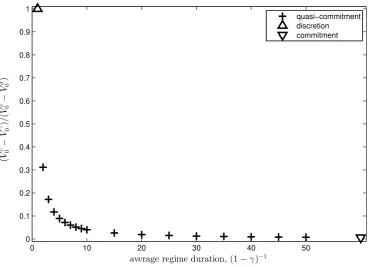
of probabilities maps into expected regime durations of {1,2,3,4, . . . ,49,50} quarters. It is clear that most of the gains from commitment accrue at low levels of credibility. According to the figure, commitments lasting just two quarters on average are sufficient to close about 70 percent of the welfare gap between full commitment and discretion. Three quarters is enough to achieve 83 percent of the total gains from commitment, while roughly 90 percent can be obtained with an expected regime duration of one year. By the two-year mark, the increments to welfare from unit increases in (1−γ)−1 are less than one percent of
Vc
0 −V0d and become negligible thereafter.
The apparent concave relationship between credibility and welfare seen here suggests that the inefficiencies of discretion, namely those resulting from the stabilization bias, can mostly be avoided with short-term policy commitments. The marginal welfare gains from long-term commitments in the deep habits model are small by comparison. These results echo the ones found by Schaumburg and Tambalotti (2007) as well as Jensen (2013) but contrast sharply with those reported in Debortoliet al. (2014). The discrepancies in this literature, however, appear to be driven primarily by differences in model choice. Where the first two employ a
28These methods refine earlier work by Roberds (1987). More recently, Debortoli and Nunes (2010) and
Debortoli, Maih, and Nunes (2014) present a similar device, which they callloose commitment, that can be used to evaluate marginal changes in credibility within a wider class of monetary and fiscal policy problems.
29Recall from (14) thatV
0=−12h1+χV˜0. It follows that (V0c−V
γ
0)/(V0c−V0d) = ( ˜V0c−V˜
γ
0)/( ˜V0c−V˜0d),
where ˜V0c and ˜V0d denote, respectively, the minimum value ˜V(x0) obtained under commitment (γ= 1) and
0 10 20 30 40 50 0
0.1 0.2 0.3 0.4 0.5 0.6 0.7 0.8 0.9 1
average regime duration, (1−γ)−1
(
V
c−0
V
γ )0
/
(
V
c−0
V
d)0
[image:26.595.114.486.87.354.2]quasi−commitment discretion commitment
Fig. 4.The welfare gap between full and quasi-commitment, expressed as a fraction of the total difference in welfare between
discretion and commitment, is depicted in the figure for average regime durations (1−γ)−1of{1,2,3,4, . . . ,49,50}quarters.
prototype sticky-price model without habit formation, the latter studies quasi-commitment using the medium-scale DSGE model of Smets and Wouters (2007).
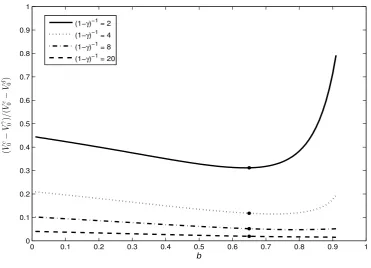
The simulations underlying Fig. 4 assume a fixed degree of habit formation b equal to 0.65. Whether these results are robust to different values of b, notably those in the upper region of the parameter space where the gains from commitment are largest, remains an open question. To that end, Fig. 5 re-graphs the welfare differentials (Vc
0 −V0γ)/(V0c −V0d)
as a function of b, holding constant (1−γ)−1 at either 2, 4, 8, or 20 quarters.
Results show that most of the gains from commitment, be they large or small, accrue at relatively low levels of credibility irrespective of the degree of habit formation. Commitments expected to last 8 quarters, for example, achieve no fewer that 90 percent of the total gains under any permissible value ofb. That threshold increases to 95 percent should commitments average 20 quarters in duration. It follows that there is little benefit to extending the period of commitment beyond a two to five-year window. Doing so would reduce the welfare gap between full and quasi-commitment by less than two percent for anyb above 0.65.
0 0.1 0.2 0.3 0.4 0.5 0.6 0.7 0.8 0.9 1 0
0.1 0.2 0.3 0.4 0.5 0.6 0.7 0.8 0.9 1
b
(
V
c−0
V
γ )0
/
(
V
c−0
V
d)0
(1−γ)−1 = 2
(1−γ)−1 = 4 (1−γ)−1 = 8
[image:27.595.114.486.87.355.2](1−γ)−1 = 20
Fig. 5.The welfare gap between full and quasi-commitment, expressed as a fraction of the total difference in welfare between
discretion and commitment, is depicted in the figure as a function of the degree of habit formationb∈(0,1) and is constructed for average regime durations (1−γ)−1
of{2,4,8,20}quarters.
appear somewhat more sensitive to the overall size of the habit externality. Consider, for example, the case in which commitments are expected to last just two quarters. Here the welfare deficit relative to full commitment increases rapidly asbapproaches its upper bound. Lifting b from 0.7 to 0.8 reduces welfare by an amount equal to 7 percent of Vc
0 − V0d.
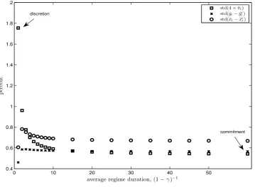
Increasingbto 0.9, however, reduces it by an additional 33 percent. At this point, monetary policy achieves less than one-third of the maximum gains available under perfect credibility. The effects of credibility on the deep habits economy can also be seen in the volatilities of the target variables featured in (10). I demonstrate this in Fig. 6 by plotting the standard deviations of (annualized) inflation, the output gap, and the habit-adjusted output gap for regime durations of {1,2,3,4, . . . ,49,50} quarters.30 Moving from discretion to a
quasi-commitment policy with two-quarter regimes cuts the standard deviation of inflation by almost half, from 1.75 to 0.96 percent. Increasing the duration of commitments to a mere six quarters brings it down to within 0.1 percentage points of the full-commitment level.
0 10 20 30 40 50 0.4
0.6 0.8 1 1.2 1.4 1.6 1.8 2
average regime duration, (1−γ)−1
p
er
ce
nt
std(4׈πt) std(ˆyt−yˆe t) std(ˆxt−xˆe
t)
discretion
[image:28.595.126.486.90.354.2]commitment
Fig. 6. Standard deviations of ˆπt (annualized), ˆyt−ˆyet, and ˆxt−xˆet under quasi-commitment are plotted for average regime
durations (1−γ)−1 of{1,2,3,4, . . . ,49,50}quarters.
Unlike inflation, however, the output gap volatilities are not monotonic with respect to credibility. In fact, the standard deviations of ˆyt−yˆte and ˆxt−xˆet reach their highest points
for average regime durations of three and two quarters, respectively. This means that the welfare gains from commitment, the bulk of which accrue at low levels of credibility, are being driven entirely by reductions in the volatility of inflation.
6
Concluding Remarks
majority of the gains can be traced to the supply-side effects that deep habits impart on the economy. This explains why the switch from discretion to commitment is accompanied by steep declines in the volatility of inflation with little change in the volatility of output.
References
Abel, Andrew B.“Asset Prices under Habit Formation and Catching Up with the Joneses.”
The American Economic Review Papers and Proceedings, May 1990, 80(2), pp. 38-42.
Amato, Jeffery D. and Laubach, Thomas. “Implications of Habit Formation for
Opti-mal Monetary Policy.” Journal of Monetary Economics, March 2004, 51(2), pp. 305-25.
Blanchard, Olivier and Gal´ı, Jordi. “Real Wage Rigidities and the New Keynesian
Model.” Journal of Money, Credit and Banking, February 2007, 39(S1), pp. 35-65.
Blinder, Alan S. Central Banking in Theory and Practice. Cambridge and London: MIT
Press, 1998.
Campbell, John Y. and Cochrane, John H.“By Force of Habit: A Consumption-Based
Explanation of Aggregate Stock Market Behavior.” Journal of Political Economy, April 1999, 107(2), pp. 205-51.
Christiano, Lawrence J.; Eichenbaum, Martin and Evans, Charles L. “Nominal
Rigidities and the Dynamic Effects of a Shock to Monetary Policy.” Journal of Political
Economy, February 2005, 113(1), pp. 1-45.
Clarida, Richard; Gal´ı, Jordi and Gertler, Mark. “The Science of Monetary Policy:
A New Keynesian Perspective.” Journal of Economic Literature, December 1999, 37(4), pp. 1661-707.
Coibion, Olivier and Gorodnichenko, Yuriy. “Strategic Interaction Among
Hetero-geneous Price-Setters in an Estimated DSGE Model.” The Review of Economics and Statistics, August 2011, 93(3), pp. 920-40.
Constantinides, George M. “Habit Formation: A Resolution of the Equity Premium
Puzzle.” Journal of Political Economy, June 1990, 98(3), pp. 519-43.
Demirel, Ufuk Devrim. “Gains from Commitment in Monetary Policy: Implications of
the Cost Channel.” Journal of Macroeconomics, December 2013, 38(B), pp. 218-26.
Dennis, Richard and S¨oderstr¨om, Ulf.“How Important is Precommitment for Monetary
Policy?” Journal of Money, Credit and Banking, June 2006, 38(4), pp. 847-72.
Debortoli, Davide and Nunes, Ricardo. “Fiscal Policy under Loose Commitment.”
Journal of Economic Theory, May 2010, 145(3), pp. 1005-32.
Debortoli, Davide; Maih, Junior and Nunes, Ricardo. “Loose Commitment in
Gal´ı, Jordi and Gertler, Mark. “Inflation Dynamics: A Structural Econometric Analy-sis.” Journal of Monetary Economics, October 1999, 44(2), pp. 195-222.
Givens, Gregory E. “A Note on Comparing Deep and Aggregate Habit Formation in
an Estimated New Keynesian Model.” Macroeconomic Dynamics, July 2015, 19(5), pp. 1148-66.
Jensen, Christian. “The Gains from Short-Term Commitments.” Journal of
Macroeco-nomics, March 2013, 35, pp. 14-23.
Justiniano, Alejandro; Primiceri, Giorgio E. and Tambalotti, Andrea.“Investment
Shocks and Business Cycles.” Journal of Monetary Economics, March 2010, 57(2), pp. 132-45.
Klein, Paul. “Using the Generalized Schur Form to Solve a Multivariate Linear
Ratio-nal Expectations Model.” Journal of Economic Dynamics and Control, September 2000, 24(10), pp. 1405-23.
Leith, Campbell; Moldovan, Ioana and Rossi, Raffaele.“Optimal Monetary Policy in
a New Keynesian Model with Habits in Consumption.” Review of Economic Dynamics, July 2012, 15(3), pp. 416-35.
Levin, Andrew T.; Onatski, Alexei; Williams, John C. and Williams, Noah.
“Mon-etary Policy Under Uncertainty in Micro-Founded Macroeconometric Models.” in Mark Gertler and Kenneth Rogoff, eds.,NBER Macroeconomics Annual 2005, Cambridge: MIT Press, 2006, pp. 229-87.
Lubik, Thomas A. and Teo, Wing Leong. “Deep Habits in the New Keynesian Phillips
Curve.” Journal of Money, Credit and Banking, February 2014, 46(1), pp. 79-114.
Marcet, Albert and Marimon, Ramon.“Recursive Contracts.” CEP Discussion Paper
No. 1055, June 2011.
Mazumder, Sandeep. “The Price-Marginal Cost Markup and its Determinants in U.S.
Manufacturing.” Macroeconomic Dynamics, June 2014, 18(4), pp. 783-811.
Ravenna, Federico and Walsh, Carl E.“Optimal Monetary Policy with the Cost
Chan-nel.” Journal of Monetary Economics, March 2006, 53(2), pp. 199-216.
Ravn, Morten; Schmitt-Groh´e, Stephanie and Uribe, Martin. “Deep Habits.”The
Review of Economic Studies, January 2006, 73(1), pp. 195-218.
Ravn, Morten O.; Schmitt-Groh´e, Stephanie; Uribe, Martin and Uuskula, Lenno.
“Deep Habits and the Dynamic Effects of Monetary Policy Shocks.” Journal of the
Roberds, William. “Models of Policy under Stochastic Replanning.” International
Eco-nomic Review, October 1987, 28(3), pp. 731-55.
Rotemberg, Julio J. “Sticky Prices in the United States.” Journal of Political Economy,
December 1982, 90(6), pp. 1187-1211.
Rotemberg, Julio J. and Woodford, Michael. “The Cyclical Behavior of Prices and
Costs.” in John B. Taylor and Michael Woodford, eds., Handbook of Macroeconomics, 1(B), Amsterdam: North-Holland, 1999, pp. 1051-135.
Rudebusch, Glenn D. and Svensson, Lars E. O. “Policy Rules for Inflation
Target-ing,” in John B. Taylor, ed., Monetary Policy Rules. Chicago and London: University of Chicago Press, 1999, pp. 203-46.
Schaumburg, Ernst and Tambalotti, Andrea. “An Investigation of the Gains from
Commitment in Monetary Policy.” Journal of Monetary Economics, March 2007, 54(2), pp. 302-24.
Smets, Frank and Wouters, Raf. “An Estimated Dynamic Stochastic General
Equilib-rium Model of the Euro Area.”Journal of the European Economic Association, September 2003, 1(5), pp. 1123-75.
. “Shocks and Frictions in US Business Cycles: A Bayesian DSGE Approach.”
The American Economic Review, June 2007, 97(3), pp. 586-606.
S¨oderlind, Paul. “Solution and Estimation of RE Macromodels With Optimal Policy.”
European Economic Review, April 1999, 43(4-6), pp. 813-23.
Woodford, Michael. Interest and Prices: Foundations of a Theory of Monetary Policy.
Princeton and Oxford: Princeton University Press, 2003.
Zubairy, Sarah. “Interest Rate Rules and Equilibrium Stability under Deep Habits.”
Macroeconomic Dynamics, January 2014a, 18(1), pp. 23-40.
. “On Fiscal Multipliers: Estimates from a Medium Scale DSGE Model.”

![Fig. 1. The percent drop in consumption (λ × 100) sufficient to equalize welfare under commitment and discretion is shownfor values of b ∈ [0, 0.94]](https://thumb-us.123doks.com/thumbv2/123dok_us/284306.527934/16.595.116.486.88.350/percent-consumption-sucient-equalize-welfare-commitment-discretion-shownfor.webp)
![Fig. 2. Standards deviations of ˆ(dashed lines) are graphed for values ofπt (annualized), ˆyt − ˆyet , and ˆxt − ˆxet obtained under commitment (solid lines) and discretion b ∈ [0, 0.94].](https://thumb-us.123doks.com/thumbv2/123dok_us/284306.527934/18.595.117.500.72.218/standards-deviations-dashed-graphed-annualized-obtained-commitment-discretion.webp)