Unsupervised Feature Learning for Visual Sign Language Identification
Binyam Gebrekidan Gebre1, Onno Crasborn2, Peter Wittenburg1, Sebastian Drude1,Tom Heskes2
1Max Planck Institute for Psycholinguistics,2Radboud University Nijmegen [email protected],[email protected],[email protected],
[email protected],[email protected]
Abstract
Prior research on language identification fo-cused primarily on text and speech. In this paper, we focus on the visual modality and present a method for identifying sign lan-guages solely from short video samples. The method is trained on unlabelled video data (un-supervised feature learning) and using these features, it is trained to discriminate between six sign languages (supervised learning). We ran experiments on short video samples in-volving 30 signers (about 6 hours in total). Us-ing leave-one-signer-out cross-validation, our evaluation shows an average best accuracy of
84%. Given that sign languages are under-resourced, unsupervised feature learning tech-niques are the right tools and our results indi-cate that this is realistic for sign language iden-tification.
1 Introduction
The task of automatic language identification is to quickly identify the identity of the language given utterances. Performing this task is key in applications involving multiple languages such as machine translation and information retrieval (e.g. metadata creation for large audiovisual archives).
Prior research on language identification is heavily biased towards written and spoken lan-guages (Dunning, 1994; Zissman, 1996; Li et al., 2007; Singer et al., 2012). While language iden-tification in signed languages is yet to be studied, significant progress has been recorded for written and spoken languages.
Written languages can be identified to about 99% accuracy using Markov models (Dunning, 1994). This accuracy is so high that current research has shifted to related more challeng-ing problems: language variety identification (Zampieri and Gebre, 2012), native language iden-tification (Tetreault et al., 2013) and ideniden-tification at the extremes of scales; many more languages,
smaller training data, shorter document lengths (Baldwin and Lui, 2010).
Spoken languages can be identified to accura-cies that range from 79-98% using different mod-els (Zissman, 1996; Singer et al., 2003). The methods used in spoken language identification have also been extended to a related class of prob-lems: native accent identification (Chen et al., 2001; Choueiter et al., 2008; Wu et al., 2010) and foreign accent identification (Teixeira et al., 1996). While some work exists on sign language recognition1 (Starner and Pentland, 1997; Starner et al., 1998; Gavrila, 1999; Cooper et al., 2012), very little research exists on sign language iden-tification except for the work by (Gebre et al., 2013), where it is shown that sign language identi-fication can be done using linguistically motivated features. Accuracies of 78% and 95% are reported on signer independent and signer dependent iden-tification of two sign languages.
This paper has two goals. First, to present a method to identify sign languages using features learned by unsupervised techniques (Hinton and Salakhutdinov, 2006; Coates et al., 2011). Sec-ond, to evaluate the method on six sign languages under different conditions.
Our contributions: a) show that unsupervised feature learning techniques, currently popular in many pattern recognition problems, also work for visual sign languages. More specifically, we show how K-means and sparse autoencoder can be used to learn features for sign language identification. b) demonstrate the impact on performance of vary-ing the number of features (aka, feature maps or filter sizes), the patch dimensions (from 2D to 3D) and the number of frames (video length).
1There is a difference between sign language recognition
and identification. Sign language recognition is the recogni-tion of the meaning of the signs in a given known sign lan-guage, whereas sign language identification is the recognition of the sign language itself from given signs.
2 The challenges in sign language identification
The challenges in sign language identification arise from three sources as described below.
2.1 Iconicity in sign languages
The relationship between forms and meanings are not totally arbitrary (Perniss et al., 2010). Both signed and spoken languages manifest iconicity, that is forms of words or signs are somehow mo-tivated by the meaning of the word or sign. While sign languages show a lot of iconicity in the lex-icon (Taub, 2001), this has not led to a universal sign language. The same concept can be iconi-cally realised by the manual articulators in a way that conforms to the phonological regularities of the languages, but still lead to different sign forms. Iconicity is also used in the morphosyntax and discourse structure of all sign languages, however, and there we see many similarities between sign languages. Both real-world and imaginary objects and locations are visualised in the space in front of the signer, and can have an impact on the artic-ulation of signs in various ways. Also, the use of constructed action appears to be used in many sign languages in similar ways. The same holds for the rich use of non-manual articulators in sentences and the limited role of facial expressions in the lexicon: these too make sign languages across the world very similar in appearance, even though the meaning of specific articulations may differ (Cras-born, 2006).
2.2 Differences between signers
Just as speakers have different voices unique to each individual, signers have also different sign-ing styles that are likely unique to each individual. Signers’ uniqueness results from how they articu-late the shapes and movements that are specified by the linguistic structure of the language. The variability between signers either in terms of phys-ical properties (hand sizes, colors, etc) or in terms of articulation (movements) is such that it does not affect the understanding of the sign language by humans, but that it may be difficult for machines to generalize over multiple individuals. At present we do not know whether the differences between signers using the same language are of a similar or different nature than the differences between dif-ferent languages. At the level of phonology, there are few differences between sign languages, but
the differences in the phonetic realization of words (their articulation) may be much larger.
2.3 Diverse environments
The visual ’activity’ of signing comes in a context of a specific environment. This environment can include the visual background and camera noises. The background objects of the video may also in-clude dynamic objects – increasing the ambiguity of signing activity. The properties and configu-rations of the camera induce variations of scale, translation, rotation, view, occlusion, etc. These variations coupled with lighting conditions may introduce noise. These challenges are by no means specific to sign interaction, and are found in many other computer vision tasks.
3 Method
Our method performs two important tasks. First, it learns a feature representation from patches of unlabelled raw video data (Hinton and Salakhut-dinov, 2006; Coates et al., 2011). Second, it looks for activations of the learned representation (by convolution) and uses these activations to learn a classifier to discriminate between sign languages.
3.1 Unsupervised feature learning
Given samples of sign language videos (unknown sign language with one signer per video), our sys-tem performs the following steps to learn a feature representation (note that these video samples are separate from the video samples that are later used for classifier learning or testing):
1. Extract patches. Extract small videos (here-after called patches) randomly from any-where in the video samples. We fix the size of the patches such that they all haver
rows, c columns and f frames and we ex-tract patches m times. This gives us X =
{x(1), x(1), . . . , x(m)}, wherex(i) ∈RN and
N =r∗c∗f (the size of a patch). For our ex-periments, we extract 100,000 patches of size
15∗15∗1(2D) and15∗15∗2(3D).
2. Normalize the patches. There is evidence that normalization and whitening (Hyv¨arinen and Oja, 2000) improve performance in un-supervised feature learning (Coates et al., 2011). We therefore normalize every patch
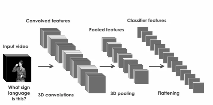
Figure 1: Illustration of feature extraction: convolution and pooling.
the standard deviation of its elements. For vi-sual data, normalization corresponds to local brightness and contrast normalization. 3. Learn a feature-mapping. Our
unsuper-vised algorithm takes in the normalized and whitened datasetX ={x(1), x(1), . . . , x(m)} and maps each input vectorx(i)to a new fea-ture vector ofK features (f : RN → RK).
We use two unsupervised learning algorithms a) K-means b) sparse autoencoders.
(a) K-means clustering: we train K-means to learns K c(k) centroids that mini-mize the distance between data points and their nearest centroids (Coates and Ng, 2012). Given the learned centroids
c(k), we measure the distance of each data point (patch) to the centroids. Natu-rally, the data points are at different tances to each centroid, we keep the dis-tances that are below the average of the distances and we set the other to zero:
fk(x) = max{0, µ(z)−zk} (1)
wherezk=||x−c(k)||2andµ(z)is the
mean of the elements ofz.
(b) Sparse autoencoder: we train a sin-gle layer autoencoder with K hid-den nodes using backpropagation to minimize squared reconstruction error. At the hidden layer, the features are mapped using a rectified linear (ReL) function (Maas et al., 2013) as follows:
f(x) =g(W x+b) (2)
whereg(z) = max(z,0). Note that ReL nodes have advantages over sigmoid or tanh functions; they create sparse repre-sentations and are suitable for naturally sparse data (Glorot et al., 2011).
From K-means, we getK RN centroids and from
the sparse autoencoder, we get W ∈ RKxN and b ∈ RK filters. We call both the centroids and
filters as the learned features.
3.2 Classifier learning
Given the learned features, the feature mapping functions and a set of labeled training videos, we extract features as follows:
1. Convolutional extraction: Extract features from equally spaced sub-patches covering the video sample.
2. Pooling: Pool features together over four non-overlapping regions of the input video to reduce the number of features. We perform max pooling for K-means and mean pooling for the sparse autoencoder over 2D regions (per frame) and over 3D regions (per all se-quence of frames).
3. Learning: Learn a linear classifier to predict the labels given the feature vectors. We use logistic regression classifier and support vec-tor machines (Pedregosa et al., 2011).
4 Experiments
4.1 Datasets
Our experimental data consist of videos of 30 signers equally divided between six sign lan-guages: British sign language (BSL), Danish (DSL), French Belgian (FBSL), Flemish (FSL), Greek (GSL), and Dutch (NGT). The data for the unsupervised feature learning comes from half of the BSL and GSL videos in the Dicta-Sign cor-pus2. Part of the other half, involving 5 signers, is used along with the other sign language videos for learning and testing classifiers.
For the unsupervised feature learning, two types of patches are created: 2D dimensions (15 ∗15) and 3D (15∗15∗2). Each type consists of ran-domly selected 100,000 patches and involves 16 different signers. For the supervised learning, 200 videos (consisting of 1 through 4 frames taken at a step of 2) are randomly sampled per sign language per signer (for a total of 6,000 samples).
4.2 Data preprocessing
The data preprocessing stage has two goals. First, to remove any non-signing signals that re-main constant within videos of a single sign lan-guage but that are different across sign lanlan-guages. For example, if the background of the videos is different across sign languages, then classifying the sign languages could be done with perfection by using signals from the background. To avoid this problem, we removed the background by us-ing background subtraction techniques and manu-ally selected thresholds.
The second reason for data preprocessing is to make the input size smaller and uniform. The videos are colored and their resolutions vary from
320∗180to720∗576. We converted the videos to grayscale and resized their heights to 144and cropped out the central144∗144patches.
4.3 Evaluation
We evaluate our system in terms of average accu-racies. We train and test our system in leave-one-signer-out cross-validation, where videos from four signers are used for training and videos of the remaining signer are used for testing. Classifica-tion algorithms are used with their default settings and the classification strategy isone-vs.-rest.
2http://www.dictasign.eu/
5 Results and Discussion
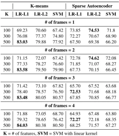
Our best average accuracy (84.03%) is obtained using 500 K-means features which are extracted over four frames (taken at a step of 2). This ac-curacy obtained for six languages is much higher than the 78% accuracy obtained for two sign lan-guages (Gebre et al., 2013). The latter uses lin-guistically motivated features that are extracted over video lengths of at least 10 seconds. Our sys-tem uses learned features that are extracted over much smaller video lengths (about half a second). All classification accuracies are presented in ta-ble 5 for 2D and tata-ble 5 for 3D. Classification con-fusions are shown in table 5. Figure 2 shows fea-tures learned by K-means and sparse autoencoder.
[image:4.595.313.508.295.408.2](a) K-means features (b) SAE features
Figure 2: All 100 features learned from 100,000 patches of size15∗15. K-means learned relatively more curving edges than the sparse auto encoder.
K-means Sparse Autoencoder K LR-L1 LR-L2 SVM LR-L1 LR-L2 SVM
# of frames = 1
100 69.23 70.60 67.42 73.85 74.53 71.8 300 76.08 77.37 74.80 72.27 70.67 68.90 500 83.03 79.88 77.92 67.50 69.38 66.20
# of frames = 2
100 71.15 72.07 67.42 72.78 74.62 72.08 300 77.33 78.27 76.60 71.85 71.07 68.27 500 83.58 79.50 79.90 67.73 70.15 66.45
# of frames = 3
100 71.42 73.10 67.82 65.70 67.52 63.68 300 78.40 78.57 76.50 72.53 71.68 68.18 500 83.48 80.05 80.57 67.85 70.85 66.77
# of frames = 4
100 71.88 73.05 68.70 64.93 67.48 63.80 300 79.32 78.65 76.42 72.27 72.18 68.35 500 84.03 80.38 80.50 68.25 71.57 67.27
K= # of features,SVM= SVM with linear kernel
LR-L?= Logistic Regression with L1 and L2 penalty
[image:4.595.319.513.477.700.2]1 2 3 4 5 6 7 8 9 10 1 2 3 4 5 6 7 8 9 10 BSL
1 2 3 4 5 6 7 8 9 10 1 2 3 4 5 6 7 8 9 10 DSL
1 2 3 4 5 6 7 8 9 10 1 2 3 4 5 6 7 8 9 10 FBSL
1 2 3 4 5 6 7 8 9 10 1 2 3 4 5 6 7 8 9 10 FSL
1 2 3 4 5 6 7 8 9 10 1 2 3 4 5 6 7 8 9 10 GSL
[image:5.595.111.477.70.254.2]1 2 3 4 5 6 7 8 9 10 1 2 3 4 5 6 7 8 9 10 NGT 0.0 0.1 0.2 0.3 0.4 0.5 0.6 0.7 0.8 0.9 1.0
Figure 3: Visualization of coefficients of Lasso (logistic regression with L1 penalty) for each sign lan-guage with respect to each of the 100 filters of the sparse autoencoder. The 100 filters are shown in figure 2(b). Each grid cell represents a frame and each filter is activated in 4 non-overlapping pooling regions.
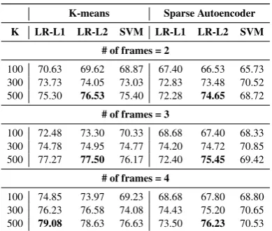
K-means Sparse Autoencoder K LR-L1 LR-L2 SVM LR-L1 LR-L2 SVM
# of frames = 2
100 70.63 69.62 68.87 67.40 66.53 65.73 300 73.73 74.05 73.03 72.83 73.48 70.52 500 75.30 76.53 75.40 72.28 74.65 68.72
# of frames = 3
100 72.48 73.30 70.33 68.68 67.40 68.33 300 74.78 74.95 74.77 74.20 74.72 70.85 500 77.27 77.50 76.17 72.40 75.45 69.42
# of frames = 4
[image:5.595.84.279.332.497.2]100 74.85 73.97 69.23 68.68 67.80 68.80 300 76.23 76.58 74.08 74.43 75.20 70.65 500 79.08 78.63 76.63 73.50 76.23 70.53
Table 2: 3D filters (15∗15∗2): Leave-one-signer-out cross-validation average accuracies.
BSL DSL FBSL FSL GSL NGT BSL 56.11 2.98 1.79 3.38 24.11 11.63
DSL 2.87 92.37 0.95 0.46 3.16 0.18
FBSL 1.48 1.96 79.04 4.69 6.62 6.21
FSL 6.96 2.96 2.06 60.81 18.15 9.07
GSL 5.50 2.55 1.67 2.57 86.05 1.65
NGT 9.08 1.33 3.98 18.76 4.41 62.44
Table 3: Confusion matrix – confusions averaged over all settings for K-means and sparse autoen-coder with 2D and 3D filters (i.e. for all # of frames, all filter sizes and all classifiers).
Tables 5 and 5 indicate that K-means performs better with 2D filters and that sparse autoencoder performs better with 3D filters. Note that features from 2D filters are pooled over each frame and
concatenated whereas, features from 3D filters are pooled over all frames.
Which filters are active for which language? Figure 3 shows visualization of the strength of fil-ter activation for each sign language. The figure shows what Lasso looks for when it identifies any of the six sign languages.
6 Conclusions and Future Work
Given that sign languages are under-resourced, unsupervised feature learning techniques are the right tools and our results show that this is realis-tic for sign language identification.
Future work can extend this work in two direc-tions: 1) by increasing the number of sign lan-guages and signers to check the stability of the learned feature activations and to relate these to iconicity and signer differences 2) by comparing our method with deep learning techniques. In our experiments, we used a single hidden layer of fea-tures, but it is worth researching into deeper layers to improve performance and gain more insight into the hierarchical composition of features.
Other questions for future work. How good are human beings at identifying sign languages? Can a machine be used to evaluate the quality of sign language interpreters by comparing them to a na-tive language model? The latter question is partic-ularly important given what happened at the Nel-son Mandela’s memorial service3.
[image:5.595.88.273.552.623.2]References
Timothy Baldwin and Marco Lui. 2010. Language identification: The long and the short of the mat-ter. In Human Language Technologies: The 2010 Annual Conference of the North American Chap-ter of the Association for Computational Linguistics, pages 229–237. Association for Computational Lin-guistics.
Tao Chen, Chao Huang, E. Chang, and Jingchun Wang. 2001. Automatic accent identification using gaus-sian mixture models. In Automatic Speech Recog-nition and Understanding, 2001. ASRU ’01. IEEE Workshop on, pages 343–346.
Ghinwa Choueiter, Geoffrey Zweig, and Patrick Nguyen. 2008. An empirical study of automatic ac-cent classification. InAcoustics, Speech and Signal Processing, 2008. ICASSP 2008. IEEE International Conference on, pages 4265–4268. IEEE.
Adam Coates and Andrew Y Ng. 2012. Learn-ing feature representations with k-means. In Neu-ral Networks: Tricks of the Trade, pages 561–580. Springer.
Adam Coates, Andrew Y Ng, and Honglak Lee. 2011. An analysis of single-layer networks in unsuper-vised feature learning. InInternational Conference on Artificial Intelligence and Statistics, pages 215– 223.
H. Cooper, E.J. Ong, N. Pugeault, and R. Bowden. 2012. Sign language recognition using sub-units.
Journal of Machine Learning Research, 13:2205– 2231.
Onno Crasborn, 2006. Nonmanual structures in sign languages, volume 8, pages 668–672. Elsevier, Ox-ford.
T. Dunning. 1994. Statistical identification of lan-guage. Computing Research Laboratory, New Mex-ico State University.
Dariu M Gavrila. 1999. The visual analysis of human movement: A survey. Computer vision and image understanding, 73(1):82–98.
Binyam Gebrekidan Gebre, Peter Wittenburg, and Tom Heskes. 2013. Automatic sign language identifica-tion. InProceedings of ICIP 2013.
Xavier Glorot, Antoine Bordes, and Yoshua Bengio. 2011. Deep sparse rectifier networks. In Proceed-ings of the 14th International Conference on Arti-ficial Intelligence and Statistics. JMLR W&CP Vol-ume, volume 15, pages 315–323.
Geoffrey E Hinton and Ruslan R Salakhutdinov. 2006. Reducing the dimensionality of data with neural net-works. Science, 313(5786):504–507.
Aapo Hyv¨arinen and Erkki Oja. 2000. Independent component analysis: algorithms and applications.
Neural networks, 13(4):411–430.
Haizhou Li, Bin Ma, and Chin-Hui Lee. 2007. A vector space modeling approach to spoken language identification. Audio, Speech, and Language Pro-cessing, IEEE Transactions on, 15(1):271–284. Andrew L Maas, Awni Y Hannun, and Andrew Y Ng.
2013. Rectifier nonlinearities improve neural net-work acoustic models. InProceedings of the ICML. Fabian Pedregosa, Ga¨el Varoquaux, Alexandre Gram-fort, Vincent Michel, Bertrand Thirion, Olivier Grisel, Mathieu Blondel, Peter Prettenhofer, Ron Weiss, Vincent Dubourg, et al. 2011. Scikit-learn: Machine learning in python. The Journal of Ma-chine Learning Research, 12:2825–2830.
Pamela Perniss, Robin L Thompson, and Gabriella Vigliocco. 2010. Iconicity as a general property of language: evidence from spoken and signed lan-guages. Frontiers in psychology, 1.
E. Singer, PA Torres-Carrasquillo, TP Gleason, WM Campbell, and D.A. Reynolds. 2003. Acous-tic, phoneAcous-tic, and discriminative approaches to auto-matic language identification. InProc. Eurospeech, volume 9.
E. Singer, P. Torres-Carrasquillo, D. Reynolds, A. Mc-Cree, F. Richardson, N. Dehak, and D. Sturim. 2012. The mitll nist lre 2011 language recogni-tion system. InOdyssey 2012-The Speaker and Lan-guage Recognition Workshop.
Thad Starner and Alex Pentland. 1997. Real-time american sign language recognition from video us-ing hidden markov models. InMotion-Based Recog-nition, pages 227–243. Springer.
Thad Starner, Joshua Weaver, and Alex Pentland. 1998. Real-time american sign language recogni-tion using desk and wearable computer based video.
IEEE Transactions on Pattern Analysis and Machine Intelligence, 20(12):1371–1375.
Sarah Taub. 2001. Language from the body: iconicity and metaphor in American Sign Language. Cam-bridge University Press, CamCam-bridge.
C. Teixeira, I. Trancoso, and A. Serralheiro. 1996. Ac-cent identification. InSpoken Language, 1996. IC-SLP 96. Proceedings., Fourth International Confer-ence on, volume 3, pages 1784–1787 vol.3.
Joel Tetreault, Daniel Blanchard, and Aoife Cahill. 2013. A report on the first native language identi-fication shared task. NAACL/HLT 2013, page 48. Tingyao Wu, Jacques Duchateau, Jean-Pierre Martens,
and Dirk Van Compernolle. 2010. Feature subset selection for improved native accent identification.
Speech Communication, 52(2):83–98.