How to Create a Monte Carlo Simulation Study using R: with Applications on Econometric Models

Munich Personal RePEc Archive

How to Create a Monte Carlo Simulation

Study using R: with Applications on

Econometric Models

Abonazel, Mohamed R.

30 December 2015

Workshop

How to Create a Monte Carlo Simulation

Study using R: with Applications on

Econometric Models

Dr. Mohamed Reda Abonazel Department of Applied Statistics and Econometrics

Summary

Contents of the workshop

1. Introduction to Monte Carlo Simulation.

2. The history of Monte Carlo methods.

3. The advantages of Monte Carlo methods.

4. The methodology of Monte Carlo methods in literatures.

5. The full steps to create a Monte Carlo simulation study (the proposed technic).

6. The Application: Multiple linear regression model with autocorrelation problem.

1.

Introduction to Monte Carlo Simulation

 Gentle (2003) defined the Monte Carlo methods, in general, are the experiments composed of random numbers to evaluate mathematical expressions

 To apply the Monte Carol method, the analyst constructs a mathematical model that simulates a real system.

 A large number of random sampling of the model is applied yielding a large number of random samples of output results from the model.

 For each sample, random data are generated on each input variable; computations are run through the model yielding random outcomes on each output variable.

2.

The history of Monte Carlo methods

 The Monte Carlo method proved to be successful and was an important instrument in the Manhattan Project. After the World War II, during the 1940s, the method was continually in use and became a prominent tool in the development of the hydrogen bomb.

 The Rand Corporation and the U.S. Air Force were two of the top organizations that were funding and circulating information on the use of the Monte Carlo method.

3.

The advantages of Monte Carlo methods

We can summarize the public advantages (goals) of Monte Carlo methods in the following points:

 Make inferences when weak statistical theory exists for an estimator

 Test null hypotheses under a variety of conditions

 Evaluate the quality of an inference method

 Evaluate the robustness of parametric inference to assumption violations

4.

The methodology of Monte Carlo methods in

literatures

Mooney (1997) presents five steps to make a Monte Carlo simulation study:

Step1: Specify the pseudo-population in symbolic terms in such a way that it can be used to generate samples by writing a code to generate data in a specific method.

Step2: Sample from the pseudo-population in ways that show the topic of interest

Step4: Repeat steps 2 and 3 t-times where t is the number of trials

Step5: Construct a relative frequency distribution of resulting values which is a Monte Carlo estimate of the sampling distribution of under the

conditions specified by the pseudo-population and the sampling procedures

5.

The proposed technic

:

The full steps to create

a Monte Carlo simulation study

 In this section, we proved the completed algorithm of Monte Carlo simulation study.

 We explain our algorithm through an application in regression framework, especially; we will use the Monte Carlo technic to prove that OLS estimators of GLR model are BLUEs.

That algorithm contents five main stages as follows:

Stage one: Planning for the study

 Satisfy our goals of the study (prove that OLS estimators of GLR model are BLUEs)

 Studying and understanding the model that will use in the study. (Studying theoretically framework of the GLR model)

The GLR model is given as:

(1)

where is dependent vector, is independent variables matrix, is unknown parameters vector, and is error term vector.

Assumptions:

A1: ( ) ( )

A3: is full column rank matrix, i.e., ( ) .

The OLS estimator of is given as:

̂ ( ) (2)

 Satisfy the simulation controls (sample size (n), number of the independent variables ( ), standard deviation of the error term ( ), theoretical assumptions of the GLR model (A1 to A3 above), and so on )

 Satisfy the criteria that will calculate in the simulation study (Bias and variance of OLS estimators, that are given as):

 Note that these criteria are given in econometric literature, but if they are not given theoretically, we can calculate them by simulation. As an example, see Abonazel (2014a), Youssef et al. (2014), and Youssef and Abonazel (2015).

Stage two: Building the model

We can build our model by generate all the simulation controls. In this stage, we must follow the following steps by order:

Step 1: Suppose any values as true values of the parameters vector .

Step 2: Choose the sample size n.

Step 4: Generate the fixed values of the independent variables matrix X under A2 and A3.

Step 5: Generate the values of dependent variable by using the regression equation, since we well know

.

Stage three: The treatment

 Once we obtain Y vector plus X matrix, thus we successes to build our model under the satisfied assumptions.

 We can summarize the treatment stage in the following steps:

Step 1: Regress Y on X by using the OLS formula in equation (2), then obtain the OLS estimations ̂ .

Step 2: Calculate the criteria that have been satisfied planning stage. Then we calculate ( ̂ ) and

( ̂ ) by using equation (3).

Stage four: The Replications

Step 1: Repeat this experiment (L-1) times, each time using the same values of the parameters and independent variables, if n and k are not changed. Of course, the u values will vary from experiment to experiment even though n and k are not changed. Therefore, in all we have L experiments, thus generating L values each of biases and variances.1

Step 2: Take the averages of these L estimates and call them Monte Carlo estimates:

( ̂ ) ∑ ̂

(4)

( ̂ ) ∑ ( ̂ )

(5)

Stage five: Evaluating and presenting the results

 After ending the treatment stage, we must check and evaluate the simulation result before put or discuss (display) it in our paper (research).

 The evaluation process aims to answer an important question: Are the results consistent with the theoretical framework or not?

 If the answer is yes, thus these results can be relied upon.

repeat the four stages with more accuracy to catch the mistake and correct it.

 The reviewing process contains two branches. First,

review the theoretical framework of the model from different books or papers. Second, review your software program, there may be programmatic mistakes.

 In the end, the results should be consistent with the theoretical framework. And then, we should display these results using a properly method.

 There are two main methods, to provide any simulation results, are tables and graphs. The researcher chooses between tables and graphs based on the contribution made by each method.

6.

The Application

:

Multiple linear regression

model with autocorrelation problem

In this application, we apply the above algorithm of Monte Carlo technic to compere between OLS and GLS estimators in multiple linear regression model when the errors are correlated with first-order autoregressive (AR(1)). In each stage, we proved R-code to create it. In this workshop, we suppose that the reader is familiar with R-programing basics. If you are not satisfied that, you can review the following references: Robert and Casella (2009), Crawley (2012), and Abonazel (2014b).

Stage one: Planning for the study

Now we apply the first stage, so we satisfy four factors as follows:

first-2. Studying theoretically framework of the model: this model is given in equation (1), where A2 and A3 are still valid, but A1 will be replaced to the following assumption:

A4: where ( ),

( ) and ( ) . The OLS and GLS estimators of under A2 to A4 are:

̂ ( ) ; ̂ ( )

where

( ) (

)

Since the elements of are usually unknowns, we develop a feasible Aitken estimator of based on consistent estimators of it:

̂ ∑ ̂_∑ ̂ ̂

̂ ∑ ̂

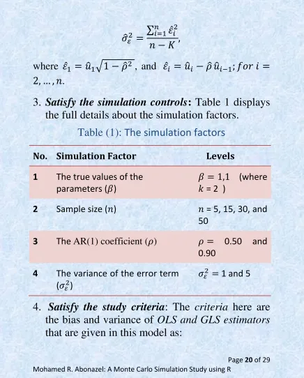
where ̂ ̂ √ ̂ , and ̂ ̂ ̂ ̂ .

3. Satisfy the simulation controls: Table 1 displays the full details about the simulation factors.

Table (1): The simulation factors

No. Simulation Factor Levels

1 The true values of the parameters ( )

(where = 2 )

2 Sample size ( ) = 5, 15, 30, and 50

3 The AR(1) coefficient ( ) 0.50 and 0.90

4 The variance of the error term ( )

1 and 5

4. Satisfy the study criteria: The criteria here are the bias and variance of OLS and GLS estimators

( ̂ ) ̂ ( ̂ ) ̂

( ̂ ) ( ) ( )

( ̂ ) ( ) Stage two: Building the model

We can build our model by generate all the simulation controls (factors) as given in table (1). The R-code is:

#---- Stage two: Building the model

#---- Step 1: Suppose the true values of the parameters vector β :

True.Beta<- c(1,1)

#---- Step 2: Choose the sample size n:

n=5

#---- Step 3: generate the random generate the of the error vector u under A1:

sigma.epsilon = sqrt(1) rho=0.50

epsilon= rnorm(n,0, sigma.epsilon) u=c(0)

u[1]=epsilon[1]/((1-(rho)^2)^0.5) for(i in 2:n) u[i]=rho*u[i-1]+epsilon[i]

#---- Step 4: Generate the fixed values of the independent variables matrix X under A2 and A3:

X = cbind(1,runif(n,-1,1))

#---- Step 5: Generate the values of dependent variable Y :

Stage three: The treatment

#---- Stage three: The treatment (by cerate estimation function): estimation<-function(Y=Y,X=X){

#---- Step 1: calculate OLS and GLS estimators

##1 ---- OLS estimator:

Beta.hat.ols = solve(t(X) %*% X) %*% t(X) %*% Y

## 2 ----GLS estimator:

rho.hat = (t(u[-n] )%*% u[-1])/sum(u[-1]^2) dim(rho.hat)=NULL

if(rho.hat>1) rho.hat=0.99; if(rho.hat<0) rho.hat=0.005 #---

epsilon.hat=NA

epsilon.hat[1]= u[1]*(1 - (rho.hat) ^2) ^0.5 epsilon.hat[2:n]= u[-1]+rho.hat * u[-n] sigma2.epsilon.hat= sum(epsilon.hat^2)/(n-2) dim(sigma2.epsilon.hat)=NULL

#---

v <- matrix(NA,nrow = n,ncol = n)

for (i in 1:n) for (j in 1:n) v[i,j] = (rho.hat) ^ abs(i - j) omega <- (sigma2.epsilon.hat / (1 - (rho.hat) ^ 2)) * v

Beta.hat.gls = solve(t(X) %*% solve(omega) %*% X) %*% (t(X) %*% solve(omega) %*% Y)

#---- Step 2: Calculate the Simulation criteria (bias and variance)

bias.ols = Beta.hat.ols - True.Beta

bias.gls = Beta.hat.gls - True.Beta

var.Beta.hat.gls = diag(solve(t(X) %*% solve(omega) %*% X))

var.Beta.hat.ols = diag (solve(t(X) %*% X) %*% t(X) %*% omega

%*% X %*% solve(t(X) %*% X))

Stage four: The Replications

Once we end the treatment stage, we obtain the values of biases and variances for only one experiment (one sample). Therefore, we Repeat this experiment (L-1) times, and then take the averages of these L estimates as follows:

#---- Stage four: The Replications L=5000

Sim.results=matrix (0,nrow=2,ncol=4)

for (l in 1:L) {

epsilon= rnorm(n,0, sigma.epsilon) u=c(0)

u[1]=epsilon[1]/((1-(rho)^2)^0.5) for(i in 2:n) u[i]=rho*u[i-1]+epsilon[i] Y=X%*%True.Beta+u

results.matrix = estimation (Y=Y,X=X) Sim.results = Sim.results + results.matrix }

average= Sim.results /l average

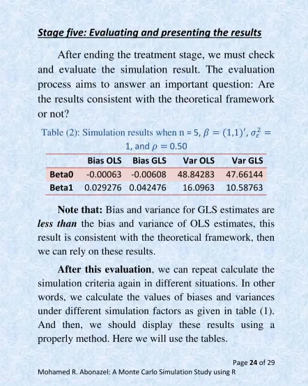
Stage five: Evaluating and presenting the results

After ending the treatment stage, we must check and evaluate the simulation result. The evaluation process aims to answer an important question: Are the results consistent with the theoretical framework or not?

Table (2): Simulation results when = 5, ( ) ,

1, and 0.50

Bias OLS Bias GLS Var OLS Var GLS

Beta0 -0.00063 -0.00608 48.84283 47.66144

Beta1 0.029276 0.042476 16.0963 10.58763

Note that: Bias and variance for GLS estimates are

less than the bias and variance of OLS estimates, this result is consistent with the theoretical framework, then we can rely on these results.

#---- Complete Program after definition our function (estimation)

###---Not Fixed--- n = c(5,15,30,50)

rho = c(0.50, 0.90)

sigma.epsilon = sqrt(c(1,5)) #---Fixed --- True.Beta <- c(1,1)

L = 1000

Sim.results = matrix (0,nrow = 2,ncol = 4) Final.table = array(NA,c(16,8))

colnames(Final.table) = c(

"n = 5","n = 5","n = 15","n = 15","n = 30","n = 30", "n = 50","n = 50")

#--- ro=0

for (rhoi in 1:2) { se = 0

for (sigma in 1:2) { sz = 0

for (ni in 1:4) {

X = cbind(1,runif(n[ni],-1,1)) for (l in 1:L) {

epsilon = rnorm(n[ni],0, sigma.epsilon[sigma]) u = c(0)

u[1] = epsilon[1] / ((1 - (rho[rhoi]) ^ 2) ^ 0.5) for (i in 2:n[ni])

u[i] = rho[rhoi] * u[i - 1] + epsilon[i] Y = X %*% True.Beta + u

results.matrix = estimation (Y = Y,X = X) Sim.results = Sim.results + results.matrix } ## for l

average = Sim.results / l

Final.table[(ro+se + 1):(ro+se + 4),(sz + 1):(sz + 2)] <- t(average) sz = sz + 2 }##for ni

se = se + 4 } ## for sigma ro=ro+8} ## for rhoi

Final.table

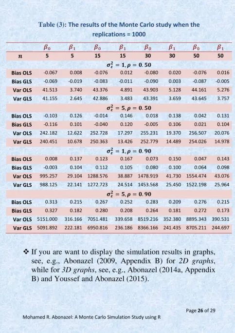
Table (3): The results of the Monte Carlo study when the replications = 1000

5 5 15 15 30 30 50 50

Bias OLS -0.067 0.008 -0.076 0.012 -0.080 0.020 -0.076 0.016

Bias GLS -0.069 -0.019 -0.083 -0.011 -0.090 0.003 -0.087 -0.005

Var OLS 41.513 3.740 43.376 4.891 43.903 5.128 44.161 5.276

Var GLS 41.155 2.645 42.886 3.483 43.391 3.659 43.645 3.757

Bias OLS -0.103 0.126 -0.014 0.146 0.018 0.138 0.042 0.131

Bias GLS -0.116 0.101 -0.040 0.120 -0.005 0.106 0.021 0.104

Var OLS 242.182 12.622 252.728 17.297 255.231 19.370 256.507 20.076

Var GLS 240.451 10.678 250.363 13.426 252.779 14.489 254.026 14.978

Bias OLS 0.008 0.137 0.123 0.167 0.073 0.150 0.047 0.143

Bias GLS -0.003 0.104 0.112 0.105 0.080 0.100 0.064 0.098

Var OLS 995.257 29.104 1288.576 38.887 1478.919 41.730 1554.474 43.076

Var GLS 988.125 22.141 1272.723 24.514 1453.568 25.450 1522.198 25.964

Bias OLS 0.313 0.215 0.267 0.252 0.283 0.209 0.276 0.215

Bias GLS 0.327 0.182 0.280 0.208 0.264 0.181 0.272 0.173

Var OLS 5151.000 316.166 7051.481 339.658 8519.216 352.380 8895.343 390.531

Var GLS 5091.892 222.181 6950.816 236.186 8366.166 241.435 8705.211 244.697

 In the previous example, we have studied the estimation properties of single-equation regression model. However there are studies are used the Monte Carlo simulation technics for multi-equation regression models (such as panel data models), see, e.g., Youssef and Abonazel (2009) and Mousa et al. (2011).

7.

General notes on simulation using R

 R is considered one of the fastest packages for

simulation.

 If the simulation time took too long or you want to end

the processing, you can press the red icon "STOP" in the tool menu anytime.

 Two way to reduce the bias (bias = mean of

experiments – true value):

o _{By increase the sample size.}

o _{By increase the number of iterations but it will}

not be as effective.

 In loops, we can create nested loops (a loop inside a

 In iterations, it is highly recommended to omit the

first 50 iterations from the calculations (such as bias or

variances values)

References

1. Abonazel, M. R. (2009). Some properties of random coefficients regression estimators. MSc thesis. Institute of Statistical Studies and Research. Cairo University.

2. Abonazel, M. R. (2014a). Some estimation methods for dynamic panel data models. PhD thesis. Institute of Statistical Studies and Research. Cairo University.

3. Abonazel, M. R. (2014b). Statistical analysis using R, Annual Conference on Statistics, Computer Sciences and Operations Research, Vol. 49. Institute of Statistical Studies and research, Cairo University. DOI: 10.13140/2.1.1427.2326.

4. Barreto, H., Howland, F. (2005). Introductory econometrics: using Monte Carlo simulation with Microsoft excel. Cambridge University Press.

5. Craft, R. K. (2003). Using spreadsheets to conduct Monte Carlo experiments for teaching introductory econometrics. Southern Economic Journal, 726-735.

6. Crawley, M. J. (2012). The R book. John Wiley & Sons.

7. Gentle, J. E. (2003). Random number generation and Monte Carlo methods. Springer Science & Business Media.

8. Gujarati, D. N. (2003) Basic econometrics. 4th ed. McGraw-Hill Education.

10.Mooney, C. Z. (1997). Monte Carlo simulation. Sage University Paper Series on Quantitative Applications in the Social Sciences, series no. 07-116. Thousand Oaks, CA: Sage.

11.Mousa, A., Youssef, A. H., Abonazel, M. R. (2011). A Monte

Carlo study for Swamy’s estimate of random coefficient panel data

model. Working paper, No. 49768. University Library of Munich, Germany.

12.Robert, C., Casella, G. (2009). Introducing Monte Carlo Methods with R. Springer Science & Business Media.

13.Robert, C., Casella, G. (2013). Monte Carlo statistical methods. Springer Science & Business Media.

14.Thomopoulos, N. T. (2012). Essentials of Monte Carlo Simulation: Statistical Methods for Building Simulation Models. Springer Science & Business Media.

15.Youssef, A. H., Abonazel, M. R. (2009). A comparative study for estimation parameters in panel data model. Working paper, No. 49713. University Library of Munich, Germany.

16.Youssef, A. H., Abonazel, M. R. (2015). Alternative GMM estimators for first-order autoregressive panel model: an improving efficiency approach. Communications in Statistics-Simulation and Computation (in press). DOI: 10.1080/03610918.2015.1073307. 17.Youssef, A. H., El-sheikh, A. A., Abonazel, M. R. (2014). New