Frequency Dependence of the Defect Sensitivity of Guided Wave Testing for Efficient Defect Detection at Pipe Elbows

Frequency Dependence of the Defect Sensitivity of Guided Wave Testing

for Ef

fi

cient Defect Detection at Pipe Elbows

Toshihiro Yamamoto

1,+

, Takashi Furukawa

1

and Hideo Nishino

2

1_{Nondestructive Evaluation Center, Japan Power Engineering and Inspection Corporation, Yokohama 230-0044, Japan} 2_{Institute of Technology and Science, the University of Tokushima, Tokushima 770-8506, Japan}

Guided wave testing offers an efficient screening method for thinning of pipe walls because of its long inspection range and its ability to inspect pipes with limited access. However, the existence of an elbow in pipes makes the interpretation of echo signals difficult. The present study investigates the sensitivity of defect detection when guided wave testing is applied to detect a defect at a pipe elbow. To examine the defect sensitivity when a defect exists at different locations on an elbow, an artificial defect was produced at one of 12 different locations on the outer surface of the elbow of each aluminum alloy piping specimen. The defect signals were observed as the defect depth was gradually increased at each defect location to obtain the defect sensitivity. The transmitted guided wave frequency was in turn set to 30 kHz, 40 kHz, and 50 kHz. At 30 kHz, high sensitivity values were obtained at the intrados of the elbows, whereas at 40 kHz and 50 kHz, high sensitivity values were obtained at their extrados. This paper also shows the results of computer simulations that used the same configuration as that used in the experiments to analyze the propagation behavior of guided waves passing through the elbow. In addition to the experimental results, the simulation results indicate that the defect-sensitive locations are controlled by the guided wave frequency. Thus, proper selection of the excitation frequency for guided wave testing enables efficient defect detection at pipe elbows. [doi:10.2320/matertrans.M2015319]

(Received November 9, 2015; Accepted December 4, 2015; Published January 18, 2016)

Keywords: nondestructive evaluation, ultrasonic testing, guided wave, pipe inspection, elbow, simulation

1. Introduction

Guided wave testing offers an efficient screening method for detecting thinning of pipe walls due to its long inspection range and ability to inspect pipes with limited access (e.g.,

covered with insulation and buried).1­8) However, the

applicability of guided wave testing for detecting defects in pipes with elbows is currently impractical due to complicated wave propagation through elbows. This problem is important for evaluating local wall thinning at pipe elbows because local wall thinning frequently occurs near elbows due to

liquid droplet impingement (LDI) erosion orflow-accelerated

corrosion (FAC).9­11)

Guided wave propagation around pipe elbows has been

studied from many viewpoints, including mode analysis12­15)

and mode conversions at elbows.16,17) Another concern

regarding guided wave testing for pipes with elbows is that waves reflected from the butt welds at both ends of an elbow produce spurious signals. Because the amplitudes of these spurious signals are much larger than those of defect signals,

defect signals may be completely obscured.18­20)

Conse-quently, masked defect signals must be extracted by some

kind of procedure, such as incremental monitoring18) _or

baseline subtraction.19,20)

Despite many studies on guided wave testing of piping that includes an elbow, the sensitivity of defect detection at the elbow has not been investigated in detail. In the present study, guided wave testing experiments were conducted using 50A Schedule 40 piping composed of aluminum alloy to examine the defect sensitivities at 12 locations around the pipe elbow at three different transmitted guided wave frequencies: 30 kHz, 40 kHz, and 50 kHz. The experimental results show that the defect sensitivity tends to be higher at the elbow intrados at 30 kHz. In contrast, it tends to be higher at the elbow extrados at 40 kHz and 50 kHz.

Computer simulations were also performed using the same configuration as that used in the experiments to analyze the propagation of guided waves passing through the elbow. The propagation of the guided waves could be observed by calculating the displacement of the outer surface of the pipe. The transient changes in the color map that depicted the magnitude distribution of the displacement caused by the guided waves helped realize the propagation behavior of the guided waves. To indicate where the displacement became relatively large during guided wave propagation using a single still image, a color map that depicted the maximum magnitude of the displacement over time at each point was used.

In the simulation results, the frequency-dependent distri-bution around the elbow exhibited by the maximum magnitude is similar to that exhibited by the experimentally derived defect sensitivity. Specifically, the displacement tends to have a larger magnitude at the elbow intrados at 30 kHz, whereas it tends to have a larger magnitude at the elbow extrados at 40 kHz and 50 kHz. This similarity between the defect sensitivity and the maximum magnitude is reasonably accepted because a high-amplitude echo signal is expected from a defect at a region where a large displacement arises. Since the computational cost of obtaining the displacement of the outer surface of a pipe is less than that of obtaining the defect sensitivity by computation, the maximum magnitude of the displacement is a convenient parameter for estimating the defect sensitivity at a certain location and a certain frequency of the transmitted guided waves.

2. Experiments to Investigate the Defect Sensitivity Characteristics at Pipe Elbows

2.1 Experimental setup

Laboratory experiments were conducted to investigate the defect sensitivity of guided wave testing applied to the detection of defects around pipe elbows. The piping used in +_{Corresponding author, E-mail: yamamoto-toshihiro@japeic.or.jp}

the experiments was made of aluminum alloy and comprised two straight pipes connected at an elbow, as shown in Fig. 1. The pipes were 50A Schedule 40 (outer diameter of 60.5 mm and wall thickness of 3.9 mm). The elbow was a long radius elbow that complied with JIS B2313 (comparable to ASME B16.9). Each end of the elbow was welded to one of the straight pipes.

The dry-coupled piezoelectric ring-shaped sensor system

presented in previous studies17,18) was used to transmit and

receive guided waves in the experiments. The sensor system comprised two sets of eight transducer elements aligned such that they were placed at equal intervals around the outer surface of the pipe. These transducer elements were oriented so that they would vibrate in the circumferential direction of the pipe to preferentially transmit and receive fundamental torsional-mode T(0, 1) guided waves. One set of the eight transducer elements was used as a transmitter, while the other set was used as a receiver. The transmitter was placed 485 mm before the inlet of the elbow and the receiver was placed 30 mm before the transmitter, as shown in Fig. 1.

Hanning window-modulated six-cycle sinusoidal tone burst signals were generated by a function generator (Tektronix AFG3102), amplified to 120 V peak-to-peak by a bipolar amplifier (NF BA4825), and fed into the transmitter.

A programmable filter (NF 3628) was employed to yield

25-fold signal amplification and to allow signals within the «10 kHz bandwidth around a given center frequency to pass through. The resulting signals were observed and captured by a digital oscilloscope (Tektronix DPO7054). Every 100 consecutive waveform samples were averaged in the oscilloscope to improve the signal-to-noise ratio

(S/N).

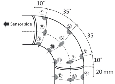
To determine the observed signal variations according to the elbow defect location, 12 piping specimens of the same configuration were prepared, as shown in Fig. 1. For each specimen, a single defect was made at one of the 12 locations presented in Fig. 2. Figure 3 shows the carbide cutting tool used to make these defects on the outer surface of the pipe wall. The diameter of the carbide cutting bit was 9.5 mm. The depth of each defect was gradually increased in 0.25 mm increments up to 2.0 mm. The observed signals were stored for each step of the defect depth on the 12 piping specimens. Three frequencies (30 kHz, 40 kHz, and 50 kHz) were applied as the center frequency of the excitation signal for the transmitter to determine how the characteristics of the observed signals changed according to the frequency of the guided waves.

2.2 Observations of defect signals

Figure 4 shows a typical waveform obtained from the measurements before a defect was made at the elbow. Signal

①is that of the guided waves propagating directly from the

transmitter to the receiver. Signal②is formed from several

wave packets reflected around the elbow. This group of wave

packets mainly comprises the two wave packets reflected

from the two butt welds at the ends of the elbow. Signal③

arises from the waves reflected by the lower right end of the piping specimen shown in Fig. 1.

485

120 2485

Receiver Transmitter

1000

Welds 30

60.

5

3.

9

(unit: mm)

Fig. 1 Schematic of the piping specimen with a piezoelectric ring-shaped sensor system.

10˚

10˚

35˚

35˚

20 mm

䐟

䐠

䐡

䐢 䐣

䐤

䐥

䐦 䐧

䐨

䐩

䐪 Sensor side

Fig. 2 Twelve locations at which artificial defects were made in elbows.

Fig. 3 Photograph of artificial defect and carbide cutting bit used to make it.

[image:2.595.330.522.71.211.2] [image:2.595.50.288.73.175.2] [image:2.595.329.523.251.389.2] [image:2.595.321.527.436.587.2]

In general, the amplitude of a signal caused by a defect is

much less than that of the spurious signal②(approximately

10% or less). In addition, the waveform of signal ② is

different for each specimen because of the irreproducibility of

welds between specimens.18­20) Since spurious signals such

as signal ② disturb or even obscure defect signals, signal

processing is necessary to extract the signal difference due to the defect. To solve this problem, incremental monitoring was suggested in Ref. 18) and the effectiveness of the baseline subtraction was studied in Ref. 19) and 20).

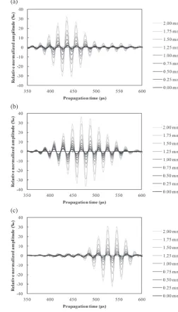
Figure 5 shows the waveforms of the observed signals with increasing defect depth when the frequency of the excitation signal was set to 50 kHz. The waveforms in Figs. 5(a), 5(b), and 5(c) were obtained when the defect was

made at locations①,②, and④, respectively; these locations

are stipulated in Fig. 2. To focus on the signal variations with defect depth, only the range from 350 µs to 600 µs is displayed. In these graphs, the signal amplitudes are normalized such that the amplitude of the signal that

corresponds to signal ① in Fig. 4 is unity for each

measurement condition. The normalized amplitudes are expressed in per mil (‰). Two overlapping wave packets

can be observed in these waveforms. The first one appears

near 400­450 µs, and the second one appears around 500­ 550 µs. These two wave packets are mainly caused by reflections from the two welds at the ends of the elbow. The amplitudes of these wave packets are different for each defect location (i.e., for each specimen) because of the differences in the welds.

The signal variations due to the defect depth increase appeared in the waveform at different times according to the defect location. In Fig. 5, signal variations are observable

around 430 µs, 480 µs, and 540 µs for defect locations①,②,

and ④, respectively. To clarify these signal variations, a

baseline subtraction method was adopted. Figures 6(a), 6(b), and 6(c) show the signals obtained by subtracting the baseline signal (the signal when the defect depth was 0 mm) from the signals in Figs. 5(a), 5(b), and 5(c), respectively. (a)

(b)

(c)

Fig. 5 Waveforms of observed signals for different defect depths at 50 kHz; (a) defect at①, (b) defect at②, (c) defect at④.

(a)

(b)

(c)

[image:3.595.54.311.70.512.2] [image:3.595.292.544.74.516.2]

Spurious signals were eliminated following subtraction, and thus, only the defect signals were extracted. For each defect location, the amplitude of the defect signal increases with the defect depth.

2.3 Defect sensitivity

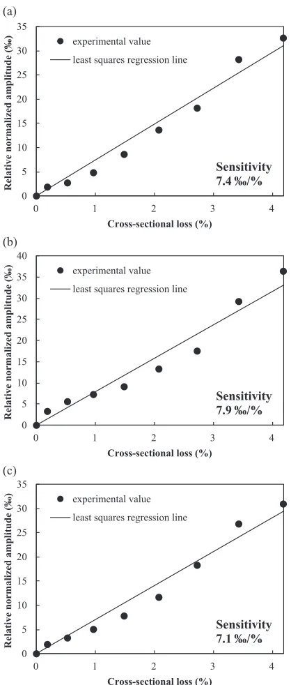
To quantify the increasing rate of the defect signal amplitude with respect to defect depth, Figs. 7(a), 7(b), and 7(c) show the correlations between the cross-sectional loss caused by the defect and the maximum amplitude of the

defect signal for defect locations①,②, and④, respectively.

In the graphs, the cross-sectional loss is represented as the

proportion (%) of the maximum cross-sectional area of the

defect to the cross-sectional area of the intact pipe wall. The

filled circles indicate the data obtained from the experiments, whereas the solid lines are the least-squares regression lines derived from the data. In this study, defect sensitivity is defined as the slope of the least-squares regression line of the correlation between the cross-sectional loss and the max-imum amplitude of the defect signal at each defect location. The measurements at the 12 piping specimens provide the defect sensitivity values at the 12 locations indicated in Fig. 2. Figure 8 shows the defect sensitivity values at these 12 locations for three frequencies: 30 kHz, 40 kHz, and 50 kHz. As shown in Fig. 8, the defect sensitivity depends on both location and frequency. For 30 kHz, higher sensitivity values are derived from the elbow intrados, whereas for 40 kHz and 50 kHz, higher sensitivity values are derived from the elbow extrados. In Fig. 9, the sensitivity values are normalized such that the defect sensitivity at a straight part of the piping is unity. The defect sensitivity at a straight part of the piping was obtained for each frequency with a 50A Schedule 40 straight pipe of aluminum alloy in the same manner as in the experiments to obtain the sensitivity at the elbow. The obtained defect sensitivities at the straight part

of the piping are 4.96‰/%, 4.76‰/%, and 6.79‰/% for

30 kHz, 40 kHz, and 50 kHz, respectively.

As shown in Fig. 9, at several locations around the elbow, the defect sensitivity is close to one, which is the defect sensitivity of the straight part of the piping. Furthermore, these sensitive locations differ depending on the guided wave frequency. For example, the defect sensitivity is nearly one at the elbow intrados for 30 kHz and at the elbow extrados for 50 kHz. This characteristic implies that appropriate frequency selection enables defect detection in the intended area of an elbow with the same sensitivity as that in a straight part of the piping. This frequency-dependent behavior of guided waves offers great potential for high-sensitivity defect detection by guided wave testing at pipe elbows.

(a) 0 5 10 15 20 25 30 35

0 1 2 3 4

Relative normalized amplitude (‰)

Cross-sectional loss (%) experimental value

least squares regression line

Sensitivity 7.4 ‰/% (b) 0 5 10 15 20 25 30 35 40

0 1 2 3 4

Relative normalized amplitude (‰)

Cross-sectional loss (%) experimental value

least squares regression line

Sensitivity 7.9 ‰/% (c) 0 5 10 15 20 25 30 35

0 1 2 3 4

Relative normalized amplitude (‰)

Cross-sectional loss (%) experimental value

least squares regression line

Sensitivity 7.1 ‰/%

Fig. 7 Correlations between cross-sectional loss caused by defect and maximum amplitude of defect signal at 50 kHz; (a) defect at①, (b) defect at②, (c) defect at④.

30 kHz Sens or s ide 2. 8 4.

1 1.4

40 kHz Sens or s ide 2. 8 3.

9 4.2

50 kHz Se nso r sid e 5. 6 4.

2 7.1

Fig. 8 Defect sensitivity (‰/%) at 12 locations at 30 kHz, 40 kHz, and 50 kHz. 30 kHz Se nso r sid e 0. 6 0.

8 0.3

40 kHz Se nso r sid e 0. 6 0.

8 0.9

50 kHz Sens or s ide 0. 8 0.

6 1.0

[image:4.595.65.274.68.559.2] [image:4.595.311.543.69.176.2] [image:4.595.312.544.218.325.2]

3. FEM Simulations to Investigate Characteristics of Guided Wave Propagation at Pipe Elbows

3.1 Configuration of FEM simulations

In the preceding section, the presented experimental results demonstrated that the defect sensitivity depends on both the defect location and the excitation signal frequency when guided wave testing is applied to detect defects at pipe elbows. This section shows the results of computer simulations conducted to determine the mechanism of this phenomenon. To conduct these simulations, the commercial simulation software ComWAVE was used.

ComWAVE, developed by ITOCHU Techno-Solutions Corporation, is ultrasonic simulation software that performs modeling, mesh generation, numerical computation, and

visualization of the results.21) _{ComWAVE employs finite}

element method (FEM) and performs computations using a finite element model developed with identical cubic elements (voxel elements). Creating a model with identical cubic elements simplifies the matrix formulation of FEM and significantly reduces computation time and memory. The time derivative of the equation to be solved is discretized by a second-order central difference scheme. Subsequently, the equation is solved explicitly.

Our group has been performing guided wave testing

simulations using ComWAVE. A previous study22)validated

the use of ComWAVE for simulations of guided waves propagating along piping by comparing the simulation results with theoretical and experimental results. This study also showed the influence of a pipe elbow on guided wave

propagation. In an experimental study,17) _{the mode}

con-versions of guided waves from the fundamental torsional mode T(0, 1) to the torsional modes T(1, 1), T(2, 1), T(3, 1), and T(4, 1) were investigated at the elbow of a piping specimen. Ring-shaped sensor systems, such as that shown in 2.1, were placed before and after the elbow and used as a transmitter and receiver, respectively. Signals received from the eight transducer elements of the receiver were used to

observe the mode conversions due to the elbow. The first

number of each mode notation, including T(1, 1), indicates the harmonic order of the vibration displacement in the circumferential direction of the pipe. The displacement direction is reversed at certain intervals along the circum-ference, and these intervals change according to the harmonic order. Subsequently, each guided wave mode was traced by analyzing the signal differences among the positions of the eight transducer elements aligned along the circumference. In Ref. 22), simulations applying the same configuration as that used in these experiments were conducted. In the simulations, the circumferential components of the displacements at the positions of the eight transducer elements were observed. The simulation results showed the same mode conversion phenomena as those observed in the experiments. In the present study, the same simulation procedure was used.

To conduct the simulations with the same configuration as that used in the experiments described in the preceding section, the shape of the specimens used in the experiments was reconstructed by combining basic geometric shapes for the simulation model. The two straight parts of the piping were modeled as hollow cylinders, and the elbow was

modeled as a quarter of a hollow torus. The weld beads at both ends of the elbow cause guided wave reflection, but they were omitted in the simulation model because they did not significantly affect the analysis results shown later in Sec. 3.2.

The specimens were made of aluminum alloy. The velocities of longitudinal and shear waves in the pipe wall

were set to 6,400 m/s and 3,120 m/s, respectively. The

density of aluminum alloy was set to 2,700 kg/m3. The

material properties were not defined in the regions other than the pipe walls. In ComWAVE, these undefined regions were

treated as perfect reflectors and computations were not

performed inside these regions to save computation time. A transmitter was placed 485 mm before the inlet of the elbow. This transmitter comprised eight vibrating blocks aligned at equal intervals in the circumferential direction of the outer surface of the pipe. All the blocks were synchronously vibrated in the same circumferential direction to generate fundamental torsional mode T(0, 1) guided waves. The displacement of each transmitter element during each time step comprised the excitation signal. The excitation signal was a Hanning window-modulated six-cycle sinus-oidal tone-burst signal with a certain center frequency. Since the aim of the simulation was to observe how guided waves propagate through an elbow, the receiver was omitted in the simulation model.

The whole simulation model was built with 0.5 mm voxels. Approximately 2 h were needed to perform the simulation for each condition via parallel computation on four processing cores of a computer with two Intel Xeon X5660 processors (2.8 GHz, six cores for each) and 32 GB of main memory.

3.2 Simulation results

Because ComWAVE calculates the output parameters during each time step, it can display the propagation of ultrasonic waves as transient changes in the magnitude distribution of the particle displacement caused by ultrasonic waves.

Figure 10(a) shows the magnitude distributions of the displacement on the outer surface of the piping at three moments when a wave packet passes through the elbow. The center frequency of the excitation signal is 50 kHz. Because the displacement has three vector components, the distribu-tions show the magnitudes of the vectors. The color changes from black to white as the magnitude increases. To indicate where the magnitude becomes relatively large using a single still image, the distribution of the maximum magnitude at each element is presented, as shown in Fig. 10(b).

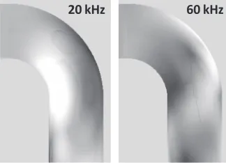
Figure 11 shows the distributions of the maximum magnitude of the displacement around the elbow when the center frequency of the excitation signal is 30 kHz, 40 kHz, and 50 kHz. These distributions reveal that the maximum magnitude of the displacement has a frequency dependence similar to that of the defect sensitivities obtained in the experiments, as shown in Fig. 9. Specifically, the maximum magnitude tends to be larger at the elbow intrados for 30 kHz, whereas it tends to be larger at the elbow extrados for 40 kHz and 50 kHz. These uneven distributions of the maximum magnitude are thought to be attributable to interference caused by guided waves at the elbow. Even if guided waves

entering the elbow are coherent, the shape of the elbow gives rise to constructive and destructive interference of the guided waves, as shown in Fig. 10(a). In this process, the wave-length of the guided waves changes how the guided waves interfere with each other. Figure 12 shows the distributions of the maximum magnitude around the elbow for 20 kHz and 60 kHz. Combined with the distributions in Fig. 11, these additional distributions support the tendency that the large displacement region is more centered at the elbow intrados for lower frequencies and more centered at the elbow extrados for higher frequencies.

For guided wave testing, a large displacement region is expected to be a defect-sensitive region. Thus, the defect sensitivity and maximum magnitude of the displacement are understood to have similar distributions. This similarity implies that the location of a defect-sensitive region is controlled by the excitation frequency and that an appropriate excitation frequency to inspect a certain region can be found from the distribution of the maximum magnitude of the

displacement obtained by the corresponding computer simulation. The calculation of the maximum magnitude of the displacement requires much less computational cost than the calculation for the defect sensitivity.

After careful inspection of Figs. 9 and 11, the defect sensitivity distributions and maximum magnitude of the displacement were determined to not match exactly. One possible reason for this difference is that the elbow was modeled as a quarter of a hollow torus in the simulation model. In reality, the wall thickness of the elbow is not constant throughout the elbow. However, it was made constant in the simulation model for simplicity. Using a more precise model may yield a better correlation. Further-more, a particular directional component of the particle displacement can be assumed to have a stronger influence on the defect sensitivity than the other components. Thus, a stronger correlation between the defect sensitivity and the particle displacement may be obtained by focusing on only a certain directional component of the particle displacement.

4. Conclusion

In our experiments, the defect sensitivity of guided wave testing at pipe elbows was investigated. Guided wave testing was performed using fundamental torsional mode T(0, 1) guided waves at three different frequencies: 30 kHz, 40 kHz, and 50 kHz. The defect sensitivity was evaluated based on the rate of increase of the maximum amplitude of the defect

signal with the cross-sectional loss of an incremental artificial

defect. An artificial defect was produced, and the size of the defect was gradually increased at one of 12 different locations on the outer surface of the elbow of a 50A Schedule 40 aluminum alloy piping specimen. The derived defect sensitivity was relatively high at the elbow intrados for 30 kHz. In contrast, it was relatively high at the elbow extrados for 40 kHz and 50 kHz. The results imply that an appropriately selected frequency enables defect detection at pipe elbows with a sensitivity high enough to be comparable to that obtained from straight pipes. Additionally, the echo signal observations showed that incremental monitoring or baseline subtraction is essential for defect detection in a pipe with an elbow. These procedures were exploited in order to extract defect signals masked by spurious signals due to the existence of an elbow.

Along with the simulation results, the experimental results indicate that the location of a defect-sensitive region can be (a)

[image:6.595.74.261.63.330.2]

(b)

Fig. 10 Simulation results for 50 kHz (black: small magnitude, white: large magnitude); (a) transient changes, (b) maximum magnitude at each element.

30 kHz 40 kHz 50 kHz

Fig. 11 Maximum magnitude distributions around the elbow at 30 kHz, 40 kHz, and 50 kHz (black: small magnitude, white: large magnitude).

[image:6.595.345.507.72.189.2]

20 kHz 60 kHz

[image:6.595.47.290.390.502.2]

controlled by adjusting the guided wave frequency when guided wave testing is applied to detect defects in pipe elbows. This fact can enable defect detection in intended regions of elbows with high sensitivity by applying an appropriate guided wave frequency. The whole elbow region can be inspected with high sensitivity using multiple frequencies. If guided wave testing is conducted using multiple frequencies, the defect may be located via the frequency at which a strong defect signal is obtained, because a strong defect signal can be obtained from a defect at the supposed location only when that frequency is used.

The locations that become defect-sensitive at a certain guided wave frequency are expected to depend upon the elbow shape and size because the mutual interference of guided waves depends on these two factors. A more detailed study of the interference of guided waves at elbows is needed to enable more accurate estimations of defect sensitivities at elbows.

Acknowledgments

This work was supported by Nuclear and Industrial Safety Agency (NISA) project on Enhancement of Ageing Manage-ment and Maintenance of Nuclear Power Plants 2010.

REFERENCES

1) D. C. Gazis:J. Acoust. Soc. Am.31(1959) 568­578.

2) A. H. Fitch:J. Acoust. Soc. Am.35(1963) 706­708.

3) D. N. Alleyne and P. Cawley:J. Nondestruct. Eval.15(1996) 11­20.

4) D. N. Alleyne and P. Cawley: Mater. Eval.55(1997) 504­508. 5) M. J. S. Lowe, D. N. Alleyne and P. Cawley:Ultrasonics36(1998)

147­154.

6) J. L. Rose: Ultrasonic Waves in Solid Media, (Cambridge University Press, Cambridge, 1990) pp. 154­175.

7) H. Kwun and K. A. Bartels:Ultrasonics36(1998) 171­178.

8) H. Nishino, S. Takashina, F. Uchida, M. Takemoto and K. Ono:Jpn. J. Appl. Phys.40(2001) 364­370.

9) J. M. Pietralik: E-J. Adv. Maintenance4(2012) 63­78.

10) N. Fujisawa, R. Morita, A. Nakamura and T. Yamagata: E-J. Adv. Maintenance4(2012) 79­87.

11) R. Morita, F. Inada, M. Sakai, S. Matsuura, S. Onishi and M. Kugimoto: E-J. Adv. Maintenance4(2012) 88­95.

12) A. Demma, P. Cawley and M. J. S. Lowe: Review of Progress in Quantitative Nondestructive Evaluation 21, ed. by D. O. Thomson and D. E. Chimenti, (Plenum, New York, 2002) pp. 157­164.

13) T. Hayashi, K. Kawashima, Z. Sun and J. L. Rose:J. Pressure Vessel Technol.127(2005) 322­327.

14) A. Demma, P. Cawley and M. J. S. Lowe: J. Pressure Vessel Technol.

127(2005) 328­335.

15) H. Nishino, K. Yoshida, H. Cho and M. Takemoto: Ultrasonics44

(2006) e1139­e1143.

16) A. Demma, P. Cawley and M. J. S. Lowe: Review of Progress in Quantitative Nondestructive Evaluation 20, ed. by D. O. Thomson and D. E. Chimenti, (Plenum, New York, 2001) pp. 172­179.

17) H. Nishino, T. Tanaka, S. Katashima and K. Yoshida: Jpn. J. Appl. Phys.50(2011) 046601.

18) H. Nishino, S. Masuda, Y. Mizobuchi, T. Asano and K. Yoshida:Jpn. J. Appl. Phys.49(2010) 116602.

19) A. Galvagni and P. Cawley: Review of Progress in Quantitative Nondestructive Evaluation 31, ed. by D. O. Thomson and D. E. Chimenti, (Plenum, New York, 2011) pp. 1591­1598.

20) A. Galvagni and P. Cawley: Review of Progress in Quantitative Nondestructive Evaluation 32, ed. by D. O. Thomson and D. E. Chimenti, (Plenum, New York, 2012) pp. 159­166.

21) Y. Ikegami, Y. Sakai and H. Nakamura: Proc. 7th Int. Conf. on NDE in Relation to Structural Integrity for Nuclear and Pressurized Compo-nents, (2009) pp. 177­190.