Improvement of Calculation Stability for Slow Fluid Flow Analysis
Using Particle Method
*Naoya Hirata and Koichi Anzai
Department of Metallurgy, Graduate School of Engineering, Tohoku University, Sendai 980–8579, Japan
MPS (Moving particle semi-implicit) method is one of the popular particle methods. It is well known that calculation instability occurs especially for a slow fluid flow analysis, and the instability appears as unnatural pressure and velocity oscillation. This is because the MPS method adopts predictor-corrector method, and tentative position of particles are not corrected enough at the corrector phase. Therefore an im-proved multiple relaxation method is proposed in this study to improve the calculation stability. Pressure and velocity correction is conducted multiply in the correction phase, and also adjusting coefficient is adopted in the source term in the Poisson equation for the pressure. As a result, the proposed method improved the pressure and velocity distribution instability. The method was applied to complex shaped casting with a shoulder. The conventional method showed unnatural high pressure and the fluid hopped, whereas smooth and natural pressure field could be obtained using the proposed method. [doi:10.2320/matertrans.F-M2016841]
(Received October 21, 2016; Accepted December 2, 2016; Published February 25, 2017)
Keywords: flow, simulation, particle method, moving particle semi-implicit (MPS) method
1. Introduction
Recently, particle methods, which are based on a fully La-grangian method, have been developing to calculate complex phenomena occurring in the casting processes1–4). Nowadays, the typical particle methods for computational continuum dy-namics are usually categorized into two methods, SPH (Smoothed Particle Hydrodynamics)2) method and MPS (Moving Particle Semi-implicit)3,4) method. Discrete objects are used as calculation elements in the particle methods, and they can be placed and moved freely in the space. This feature allows the particle methods to simulate the heat and mass transfer phenomena that are observed in the casting process more easily and directly than other methods that use the cal-culation lattice.
However, the particle methods have still some problems. Calculation stability is one of the significant problems in the particle methods. Casting process involves a variety of phe-nomena which occur simultaneously from the pouring to the solidification. Because it is difficult to expect what kind of phenomena will occur at where and at which timing, higher calculation stability is required for the integrated simulation using particle methods. It is known that the oscillation of ve-locity and pressure occurs in the flow simulation, and the os-cillation decreases the calculation stability especially for a slow flow5). Hirata et al. have proposed a stable and rapid calculation method for the slow flow by ignoring inertia force and adjusting the gravitational force after the fluid flow can be assumed to be almost stopped5). However, the procedure requires precise estimation of the flow stop time. The original flow calculation by the particle method3) is unstable for the slow fluid flow. Therefore the flow calculation without any improvement will decrease the calculation stability when the flow becomes slow during the casting processes. Recently, Hirata et al. reported the multiple relaxation method which improves calculation stability and speed6) in the case of slow
fluid flow. However, the oscillation of pressure and velocity are still not negligible. Therefore further improvement in the accuracy is expected. In this study, we tried further improve-ment of the calculation stability and accuracy of the particle method in the case of slow fluid flow by improving the multi-ple relaxation method.
2. Numerical Method
We adopted MPS method to combine flow and solidifica-tion simulasolidifica-tions. In the MPS method, the calculasolidifica-tions such as gradient operation are evaluated by calculating an interaction among the surrounding particles. The interaction is calculated with the particles by weighted averaging within a certain dis-tance, which is referred to as the kernel size. A summary of the proposed calculation algorithms is shown in this section.
2.1 Weight function and particle interaction models
A weight function w is used in the MPS method to calcu-late the interaction of particles by weighted averaging. Equa-tion (1) was used in this study because of its higher stability for the flow calculation7).
w(r,ckr0)
= 40 7πck2
1−c6r2
k2r02 +
6r3
ck3r03 (0≤r<0.5ckr0)
10 7πck2
2−c2r
kr0
3
(0.5ckr0≤r<ckr0)
0 (ckr0<r)
(1)
Here, r is a distance between particles i and j. ckr0 is the kernel size which represents interaction calculation range. The MPS method uses particle size r0 which has the same significance as the lattice size in the Eulerian methods such as FDM (finite difference method). ck is the kernel size coeffi-cient and usually varies between 2 and 4. ck = 2.1 was used in this study as a commonly used value3,7).
Particle number density ni of the particle i is used in the particle method to calculate the interaction between particle i *
This Paper was Originally Published in Japanese in J. JFS. 87 (2015) 702– 708.
and the surrounding particles. ni is the sum of the weight function of the particles surrounding the particle i, and is ex-pressed as follows.
ni= i j
w rj−ri ,ckr0 (2)
Here, ri and rj are the position vectors of particle i and j, respectively. Assuming that the fluid is incompressible and considering that the particle number density is directly related to the fluid density, ni is equal to n0 in the case that a particle has no surface particle around it. And we can use n0 for the mass conservation condition in the incompressible fluid flow analysis using the MPS method.
Particle interaction models are used to describe the differ-ential operators in the MPS method. If ϕi and ϕj are arbitrary scalars at positions ri and rj, then the particle interaction mod-els for the differential operators at the particle i can be ex-pressed as follows.
∇φi= d
ni i j
(φi−φj) rj−ri ·
(rj−ri) rj−ri
w rj−ri ,ckr0 (3)
∇2φi= 2d
ni i j
(φi−φj) rj−ri2
w rj−ri ,ckr0 (4)
Equation (3) is a gradient model, and eq. (4) is a Laplacian model. Suffixes i and j represent the assigned numbers of par-ticles. The d is the number of space dimensions.
2.2 Flow simulation
The governing equations for incompressible flow calcula-tion by the MPS method consist of the continuity equacalcula-tion and the Navier-Stokes equation as follows.
Dρ
Dt =0, Du
Dt =−
1
ρ∇p+ν∇
2u+f (5)
Here, ρ indicates density (kg/m3); u, velocity vector (m/s); p, pressure (Pa); ν, kinematic viscosity (m2/s); and f (m/s2), the body force acceleration vector including gravity. The left-hand side of the second equation, D/Dt, is the Lagrangian derivative, having the same significance as temporal differen-tiation.
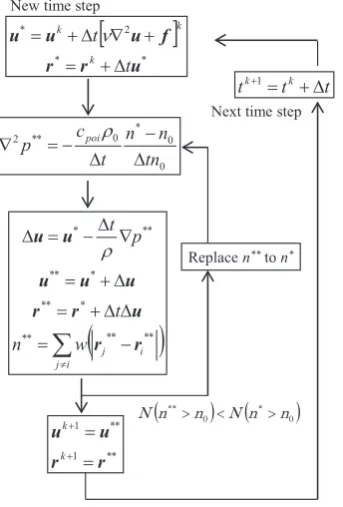
Flow calculation by the MPS method is based on the pre-dictor-corrector method similar to that in the case of the FDM or other Eulerian methods. The major differences between the MPS method and the FDM are the formulation of the Poisson equation of pressure and the calculation of particle position. In the MPS method, the tentative particle position is calculat-ed using tentative velocity in the prcalculat-ediction phase. Therefore, the correction in position is calculated along with the correc-tion in velocity in the correccorrec-tion phase. The Poisson equacorrec-tion for pressure in the MPS method is described using the tenta-tive particle number density n* and n0 as follows1).
∇2pk+1=− ρ
∆t2
n∗−n 0
n0 (6)
Here, n* is the tentative particle number density calculated using the tentative particle positions r* and eq. (2).
In the MPS method, the pressure is calculated so as to make the tentative particle number density n* to the constant
value n0, whereas making the divergence of velocity to zero in the FDM.
In the flow simulation with a free surface, the pressure at the free surface is assumed to be zero. The criteria to deter-mine the free surface particles is described as following equa-tion because the particle number density decrease at the free surface.
ni
n0 < β (7)
β = 0.97 is usually used in the MPS method with a different weight function to the eq. (1)3). In this study, β = 0.985 was used for eq. (1), which shows the most natural free surface particle criteria.
The time increment Δt is calculated by using Courant num-ber Cn using the following equation.
∆t=Cn r0
|umax| (8) Here, umax is the maximum velocity of the particles. It is
known that the use of small Δt sometimes worsens the calcu-lation stability. This is because the source term of the Poisson equation includes Δt2 in its denominator, and too small Δt produces unnatural high pressure. In this study, constant val-ue Cn = 0.1 was used.
3. Improvement of Calculation Stability for Slow Fluid Flow
The authors have reported that the multiple relaxation method improves calculation stability and speed in the previ-ous report6). However unnatural pressure oscillation and un-natural movement of the surface particle are still at issues. Pressure oscillation should be avoided as far as possible to predict a feeding behavior to the solidification shrinkage pre-cisely. Therefore an improved multiple relaxation method was proposed in this study to avoid unnatural pressure oscil-lation.
3.1 Improved multiple relaxation method
the expected position without excess movement. The flow-chart for the flow simulation with the improved multiple re-laxation method is shown in the Fig. 1. The Poisson equation is solved more than once in the multiple relaxation method. Accordingly the velocity and position are also corrected more than once during one time step. The improved method uses the adjustment coefficient cpoi in the source term in the Pois-son equation for the pressure.
3.2 Calculation model
Two-dimensional flow calculation is conducted for still flu-id as shown in the Fig. 2. The wflu-idth of casting (fluflu-id) is 40 mm and the height is 80 mm. Particle size is 2 mm; thus, we use 800 particles for the casting, 384 particles for the mold. The calculation is conducted for 2 seconds. The maxi-mum time increment Δtmax, the number of multiple relax-ations (MR) and the adjustment coefficient in the source term of the Poisson equation cpoi, and the pressure value at three
points were measured. The measuring points were at the cen-ter in the horizontal directions and the depth from the casting surface were h = 30, 50 70 mm. The physical properties and the calculation conditions are shown in Table 1 and 2. The relationship between Δtmax and the number of multiple relax-ation is determined to optimize the stability and the efficiency of calculation referring the past research6). Four c
poi values (cpoi = 1.0, 0.5, 0.2, 0.1) were used for each MR and Δtmax conditions.
3.3 Results 3.3.1 Pressure
Figure 3 shows a pressure distribution at 0.1 s. From now on, the calculation conditions are expressed using the combi-nation of the number of multiple relaxation and cpoi; for ex-ample, in the case of two times of multiple relaxation and cpoi = 0.5, the condition is expressed as MR2-0.5. An ideal hydrostatic pressure at the bottom of the casting is 1960 Pa. Figure 3(a) is the result in the case of the basic MPS method without multiple relaxations and cpoi = 1.0. The pressure dis-tribution was non-uniform, and the maximum value exceeded 5000 Pa. Such non-uniform distribution was not settled during 2 s calculation, and the particles continued to flow in Fig. 1 Flow chart for the flow simulation.
Fig. 2 Calculation model.
Table 2 Calculation condition.
Δtmax (s) MR (Multiple relaxation) cpoi
0.0001 1 1.0
0.0005 2 0.5
0.001 5 0.2
0.002 10 0.1
[image:3.595.86.258.71.325.2]Fig. 3 Pressure distribution at 0.1 s. Table 1 Physical properties for simulation.
Casting
Materials Pure Al
Density, kg/m3 2500
[image:3.595.318.536.227.462.2] [image:3.595.65.268.369.529.2]whole unnaturally. Figure 3(b) is the result in the case of two times multiple relaxations with cpoi = 1.0. The pressure at the bottom was around 2000 Pa which is similar to the ideal val-ue, however remains non-uniform distribution. Figure 3(c) is the results in the case of five times multiple relaxations and cpoi = 0.5. In this case, significant improvement was found compared with the former two results. We could obtain al-most similar results under the conditions shown in the Ta-ble 2, except for MR1-1.0 and MR2-1.0 as shown in the Fig. 3(a) and (b).
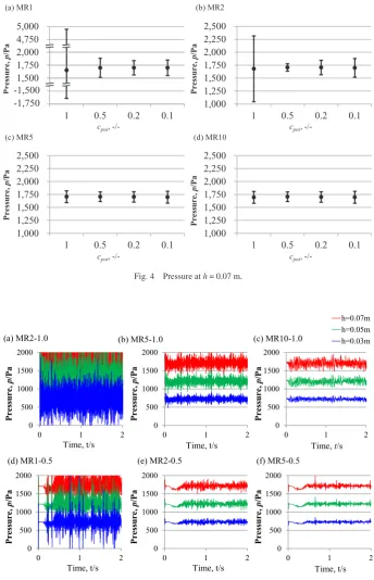
Next, an average pressure value during 2 s at h = 70 mm and a standard deviation of the pressure are shown in the
Fig. 4. Black dots are the average value and the error bars correspond to the standard deviation. The ideal pressure value at h = 70 mm is 1715 Pa. The average values indicated by the black dots agreed well with the ideal value in each condition. On the other hand, the standard deviation of MR1-1.0 and MR2-1.0 were larger than the other conditions, showing a similar tendency in the Fig. 3. As a result, the ideal pressure distribution could be achieved in the case that the standard deviation was less than 200 Pa in this study.
For further discussion, the pressure change in time under typical six conditions are shown in Fig. 5. The figures show the pressure oscillation at h = 30, 50, 70 mm. Figure 5(a) to
Fig. 4 Pressure at h = 0.07 m.
[image:4.595.124.469.242.777.2](c) show the results in the case of cpoi = 1.0. The results show that the multiple relaxation reduced the pressure oscillation, and the effect was more obvious if the number of multiple relaxations is higher. Figure 5(d) to (f) are the case of cpoi = 0.5. Figure 5(d) shows that the pressure oscillation could not be reduced enough without multiple relaxations. From the Fig. 5(e) and (f), the combination of the multiple relaxations and adjustment coefficient cpoi significantly reduces the pres-sure oscillation.
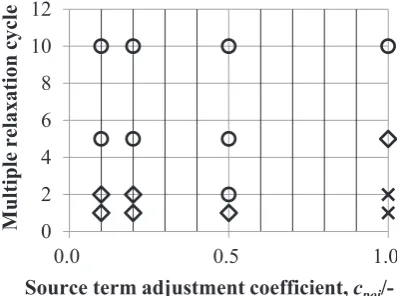
A relationship between calculation conditions and the fluid behavior was summarized in Fig. 6. The circle indicates the conditions showing the excellent stability of still fluid with less pressure oscillation. Cross mark means poor stability conditions which show an unnatural rapid increase of pres-sure, and the calculation resulted in failure with a divergence of the velocity field. Diamond shows the conditions which do not result in failure, however, unnatural behavior such as hop-ping of fluid occurs. Overall, a use of multiple relaxations and less cpoi conditions improved calculation stability. Whereas in the case of 2 times multiple relaxations, too small cpoi could reduce the stability. This is because 2 times multiple relax-ations is not enough for pressure, velocity and positional cor-rection in the corcor-rection phase if cpoi is too small.
3.3.2 Velocity
Figure 7 shows a variation of the maximum velocity of par-ticles. Figure 7(a) and (b) are the results in the case of MR1 and MR5, respectively. The results in the case of MR2 and MR10 were similar to the case of MR5. In the case without multiple relaxations shown in the Fig. 7(a), the use of smaller cpoi decrease the maximum velocity, whereas the values were larger than any case with multiple relaxations shown in the Fig. 7(b). However, the maximum velocity was over 0.05 m/s and the average velocity was over 0.02 m/s even using the multiple relaxations. Therefore, if the maximum or average velocity is expected to be under such values, some artificial operation will be useful; such as ignoring the inertia force of fluid particles after pouring as reported by Hirata et al.5)
3.3.3 Pressure stability in complex shaped casting
Finally, we discuss the pressure stability in the complex shaped casting. In this section, three-dimensional flow calcu-lation was conducted for a cylindrical casting with a shoulder.
Fig. 7 Maximum velocity of particles.
Fig. 6 Effect of multiple relaxation and source term adjustment on the pres-sure stability of the flow simulation for gently placed fluid. Circle indi-cates excellent stability, diamond shows good stability but large
[image:5.595.326.524.71.415.2] [image:5.595.324.521.76.764.2] [image:5.595.336.512.399.769.2] [image:5.595.68.267.591.739.2]The height of the casting was 180 mm, and the upper half of the casting was 25 mm and the lower half was 40 mm in di-ameter, respectively. The physical properties used in the cal-culation are shown in the Table 1, and the fluid was poured from the upper side with a rate of 100 g/s and pouring finish within 4 s. The results are shown in the Fig. 8. Figure 8(a) is the result of MR1-1.0 at 4.5 s, showing unnatural pressure distribution at the bottom of the casting, and hopping of the casting particles. At the last moment, the fluid flow was very slow. However the pressure in the casting was unnaturally high under the shoulder. In such shapes with shoulders, posi-tional correction in the correction phase tends to be insuffi-cient, and the pressure under the shoulder will be accumulat-ed unnaturally. As a result, unnatural hopping occurs, and the calculation will result in failure. In the Fig. 8(b), we can find that the proposed method improves the calculation stability. The calculated pressure value at the bottom agreed well with the theoretical value, 4410 Pa. It is possible to improve calcu-lation stability by using smaller Δt. However the pressure or velocity oscillation problem will remain, and also, longer cal-culation time will be required because of higher maximum velocity.
The series of results show that the multiple relaxation method and the use of adjustment coefficient cpoi are effective to reduce unnatural oscillation of the pressure and the veloci-ty, and to improve calculation stability for slow fluid flow, even for the complex shaped casting with the shoulder. Im-proved multiple relaxation method can improve the unnatural velocity decay and calculation stability for faster fluid flow.
The results of the faster flow calculation are discussed in the next report8).
4. Conclusions
The improved multiple relaxation method was proposed to improve calculation stability for slow fluid flow based on the MPS method; one of the particle methods. The multiple re-laxation method is combined with the adjustment coefficient of the source term in the Poisson equation of pressure. As a result, the pressure oscillation was significantly reduced by the proposed method, and the calculation stability was also improved. The proposed method can calculate stably even for the complex shaped casting with the shoulder.
Acknowledgement
The authors wish to thank the young researchers support program 2012 of JFS for its support.
REFERENCES
1) S.Koshizuka: Suuchi Ryutai Rikigaku, (Baifukan, 1997). 2) S. Koshizuka: Ryushihou Simulation, (Baifukan, 2008). 3) S. Koshizuka: Ryushihou, (Maruzen, 2005).
4) S. Koshizuka:, Ryushihou Nyumon, (Maruzen, 2014). 5) N. Hirata and K. Anzai: Mater. Trans. 52 (2011) 1931–1938. 6) N. Hirata and K. Anzai: J.JFS 86 (2014) 127.