Evaluating Spatial Distribution Randomness of Overlap Permissive
Second Phase in Three- and Two-Dimensions
Kenjiro Sugio
*1, Yasutaka Momota
*2, Di Zhang
*2, Hiroshi Fukushima and Osamu Yanagisawa
Mechanical System Engineering, Graduate School of Engineering, Hiroshima University, Higashi-Hiroshima 739-8527, Japan
Three-dimensional local number, LN3D, and two-dimensional local number, LN2D, were defined as the number of gravity centers (GCs) of second phase particles in the measuring sphere and circle with specially determined radiuses, respectively, whose centers were put on GCs of noticed particles. LN3D and LN2D represent local number density including a noticed and its neighboring particles and each particle has a specific value. We suggested the quantitative method to evaluate the particle spatial distribution using the relative frequency distributions of LN3D and LN2D, and this method was examined by computer experiments using overlap permissive spheres. It was shown that randomness of second phase particles was correctly evaluated in 3- and 2-dimensions by this method, and the average and variance of LN3D and LN2D are proper descriptors to evaluate the spatial distribution randomness of second phase particles. It was also shown that spatial distribution randomness of 2-dimensional particles appeared on cut planes of 3-dimensional particles having uniform random arrangement can be evaluated by this method regardless of both the particle volume fraction and the particle size distribution. [doi:10.2320/matertrans.MER2007125]
(Received June 4, 2007; Accepted August 10, 2007; Published September 12, 2007)
Keywords: spatial distribution, randomness, second phase, particle reinforced metal matrix composite, computer experiment
1. Introduction
Particle reinforced metal matrix composites (PMMCs) are now emerging as an important class of engineering materials due to their superior mechanical properties and amenability to the conventional metal working processes. Over the last decade, experimental and numerical studies1–11) have been indicated that the spatial distribution of second phase particles played an important role on the mechanical proper-ties. Tessellation techniques,12,13)correlation functions,14–16) nearest neighbor distances17–19) contact distribution20) and counting methods21) have been suggested to describe the spatial distribution of second phase particles. However, the developments of techniques for characterizing the spatial distribution of second phase particles have not been enough. The descriptors for the spatial distribution of particles have to be sensitive to their arrangements. Simple scalar descrip-tors such as volume fraction have been successful in understanding and predicting material behaviors of PMMCs using the simple formula, ‘rule of mixtures’. Therefore, simple scalar descriptors for the spatial distribution, which links to material behaviors, are desired.
In general, the spatial distribution of second phase particles is experimentally evaluated in 2-dimension by analyzing scanning electron microscope (SEM) or optical microscope (OM) images. The spatial distribution in 3-dimension has been also evaluated by serial sectioning method10,22) or synchrotron X-ray micro-tomography,23) but these tech-niques are not common. Computer modeling is a powerful tool for analyzing the spatial distribution of second phase particles in 3-dimension, and some researchers14–17,24) have investigated the statistical relationship between 3- and 2-dimensional spatial distributions. If the simple statistical relationship between 3- and 2-dimensional spatial distribu-tions is derived, material behaviors of PMMCs may be
predicted only by the 2-dimensional spatial distribution, which is evaluated by analyzing SEM or OM images.
We have employed the average of 2-dimensional local number, LN2D, as a spatial distribution descriptor for aluminum–silicon carbide (Al-SiC) composites, and indicat-ed that this descriptor was sensitive to the spatial distribution of second phase particles.25)We have also investigated the relation between the average of LN2D and tensile behavior. However, the formulation of this relation has not been completed because statistical properties of LN2D have not been interpreted.
In the present work, we have individually defined 3-dimensional local number, LN3D, and 2-3-dimensional local number, LN2D, and suggested the quantitative method to evaluate the particle spatial distribution using the relative frequency distributions of LN3D and LN2D. This method was examined by computer experiments using overlap permissive spheres of uniform random arrangement.
2. Procedure of Computer Experiments
2.1 Definitions of LN3D and LN2D
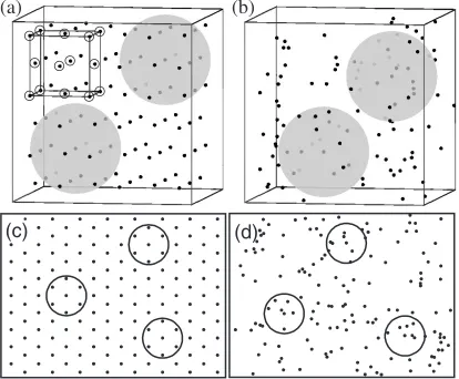
At first, let us assume that gravity centers (GCs) of second phase particles are arranged in the closed-packed, face-centered, structure in 3-dimension as shown in Fig. 1(a). We defined the measuring sphere with center at GC of a noticed particle and a radius, R3D, whereR3D is given so that the measuring sphere includes GCs of the nearest neighbor particles. In this definition, the number of GCs included in the measuring sphere is equal to 13 and the number density per unit volume is equal to13=ð4R3D3=3Þ. Then, the measuring radius,R3D, is determined so that the number density of the measuring spheres is equal to the whole number density,V, andR3Dis represented by
13
4R3D3=3
¼V )R3D¼ 13
4V=3
1=3
¼1:459
V1=3
: ð1Þ
*1Corresponding author, E-mail: [email protected]
In the present work, the number of GCs included in the measuring sphere with the radius, R3D, is defined as 3-dimensional local number, LN3D. When GCs are randomly distributed with keeping the number densityV, the identical measuring sphere with the radius,R3D, is used for measure-ments as shown in Fig. 1(b), putting the centers of measuring sphere on GCs of particles.
Secondly, let us assume that GCs of second phase particles are arranged in the closest hexagonal structure in 2-dimension as shown in Fig. 1(c). We defined the measuring circle with center at GC of a noticed particle and a radius, R2D, whereR2Dis given so that the measuring circle includes GCs of nearest neighbor particles. In this definition, the number of GCs included in the measuring circle is equal to 7 and the number density per unit area is equal to 7=R2D2. Then, the measuring radius, R2D, is determined so that the number density of the measuring circle is equal to the whole number density,A, andR2Dis represented by
7
R2D2
¼A)R2D¼ 7
A
1=2
¼1:493
A1=2
: ð2Þ
In the present work, the number of GCs included in the measuring circle with radius, R2D, is defined as 2-dimen-sional local number, LN2D. When GCs are randomly distributed with keeping the number densityA, the identical measuring sphere with the radius,R2D, is used for measure-ments as shown in Fig. 1(d).
Since the center of the measuring window (sphere and circle) is located at GCs of particles both in 3- and 2-dimensions, each particle has one specific value of LN3D or LN2D, which is regarded as one of characteristics of a noticed particle similar to particle-size or particle-shape factor and so on. Then we consider that the evaluation of spatial distribution is possible by observing the frequency distributions of LN3D or LN2D as well as using size distribution to characterize the over all particle character-istics, for example.
2.2 Measurements of LN3D and LN2D
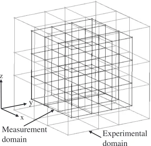
Figure 2 shows the 3-dimensional computational space to arrange second phase particles. In order to eliminate errors close to the outer surfaces of the space, this computational space consists of the measurement- and the experimental domain. The measurement domain is included in the experimental domain. The size of the measurement domain is L0L0L0, where L0 is non-dimensional length. The
size of the experimental domain was extended to ensure that the measuring spheres and circles on cut planes stayed within the experimental domain. The extended length was 1.2 times as large as the radius of the measuring sphere. Since the particles were distributed in the experimental domain but LN3D and LN2D were measured only for the noticed GCs in the measurement domain, this extension could eliminate errors near surfaces.
(c)
(d)
(b)
(a)
[image:2.595.92.506.77.419.2]We assumed that the shape of second phase particles was spherical and overlaps of particles were permitted. The number of second phase particles in the measurement domain, N0, was set at 6000 as setting value. The GCs of
second phase particles were positioned randomly in the experimental domain including the measurement domain by computer-generated random number, keeping the number densityN0=L03.
Three kinds of particle diameter,d0, and three kinds of size
distribution were evaluated as shown in Table 1, where d0 was given by the extended volume fraction, overlap
permissive volume fraction,
Vex¼
4
3
d0
2
3
N0=L03)d0 ¼L0
6Vex
N0
1=3 : ð3Þ
The shape of size distribution is shown in Fig. 3. The size distribution 1 (SID 1) is the mono-sized distribution and the diameter of all particles is set atd0. The size distributions 2
and 3 (SID 2 and SID 3) have eleven classes of particle diameters, and the particle diameters are varied linearly. The maximum and the minimum diameters were set at1:9d0and
0:1d0, respectively. The particle numbers of each class are
also varied linearly, and the maximum and the minimum particle numbers were set at 1:9N0=11 and 0:1N0=11,
respectively. Nine models (Model 1–Model 9) were totally evaluated in the present calculation, changing Vex and size distribution as shown in Table 1.
Figures 4(a) and (b) show the particle configurations of Model 2 and Model 8. Mono-sized particles are randomly distributed in Fig. 4(a) and poly-dispersed particles are randomly distributed in Fig. 4(b).
The measurement of LN3D was carried out in two iterations. In the first iteration, total number of GCs of second phase particles included in the measurement domain, NV, was counted. Whole number density per unit volume,V, was calculated byV ¼NV=L03, andR3Dwas calculated by eq. (1). In the second iteration, measuring sphere with the radius,R3D, was defined, and GCs included in each measur-ing sphere, whose center was positioned at the noticed GC, were counted.
A given volume is not necessary in the measurement of LN3D because LN3D is measured only by GCs of second phase particles. Three series of the particle configurations (Config 1, Config 2 and Config 3) with different seeds of random number were evaluated in the present calculation. Because about 6000 data of LN3D were obtained in one calculation and eleven calculations were carried out for each series changing the seed of random number, data of LN3D more than 60000 were collected for each series. Then, the relative frequency distribution of LN3D was obtained finally. When Model 2 and Model 8 are cut by arbitrary planes, circles appear on the cut planes as shown in Figs. 4(c) and (d). We used these planes to measure LN2D. The measure-ment of LN2D was also carried out in two iterations. In the first iteration, total number of GCs of circles on cut planes, NA, and total area of cut planes,A, was measured, changing positions and normal vectors of cut planes randomly. Whole number density per unit area, A, was calculated by
A¼NA=A, andR2Dwas calculated by eq. (2). In the second iteration, measuring circles with the radius,R2D, were defined for all GCs of circles on cut planes and GCs included in each measuring circle, whose center was positioned at the noticed GC, were counted. Positions and normal vectors of cut planes
x
y
z
Experimental
domain
Measurement
domain
Fig. 2 The 3-dimensional computational space to arrange second phase particles.
Table 1 Nine models evaluated in the present calculation.
Extended volume fraction,Vex
Particle
diameter,d0 Size distribution
Model 1 0.01 0.015L0 SID 1
Model 2 0.4 0.05L0 SID 1
Model 3 3.14 0.1L0 SID 1
Model 4 0.01 0.015L0 SID 2
Model 5 0.4 0.05L0 SID 2
Model 6 3.14 0.1L0 SID 2
Model 7 0.01 0.015L0 SID 3
Model 8 0.4 0.05L0 SID 3
Model 9 3.14 0.1L0 SID 3
0.0 0.0 0.2 0.4 0.6 0.8 1.0 1.2 1.4 1.6 1.8 2.0
d0
Ratio of par
ticle n
umber
Ratio of particle size
SID 1 SID 2 SID 3
1.8 1.6 1.4 1.2 1.0 0.8 0.6 0.4 0.2
[image:3.595.50.290.72.305.2] [image:3.595.312.542.75.257.2]used in the second iteration were identical to those in the first iteration.
A volume is necessary for the measurement of LN2D. If particles don’t have a volume, circles will not appear on cut planes. As shown in Table 1, nine models were evaluated in the present calculation so as to investigate the effect of the particle volume on the relative frequency distribution of LN2D. The identical particle configuration in 3-dimension, Config 1, is employed for all models. Because about 6000 data of LN2D were obtained in one calculation and eleven calculations were carried out for each model, data of LN2D more than 60000 were collected for each model. Then, the relative frequency distribution of LN2D was obtained finally.
3. Results and Discussion
3.1 Relative frequency distribution of LN3D
When the points are randomly distributed in 3-dimansion, the number of points in a window whose volume is WV at arbitrary position is Poisson distributed.26)Probability of the
point number,k, is represented by
PðkÞ ¼ðVWVÞ
k
k! expðVWVÞ k¼0;1;2 : ð4Þ
In the measurement of LN3D, we have defined so that the measuring sphere has the volume of WV ¼4R3D3=3, and then VWV ¼13 using eq. (1). When the centers of the measuring sphere are put on GCs of all particles, the measuring spheres always include one GC. Therefore, Poisson distribution shifts to the larger LN3D by 1, and we can expect that the probability of LN3D is represented by
PðLN3D¼kþ1Þ ¼13
k
k! expð13Þ k¼0;1;2 : ð5Þ
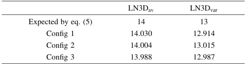
The average and the variance of this modified Poisson distribution are 14 and 13, respectively. Figure 5 shows the probability distribution of eq. (5) and the relative frequency distributions of LN3D measured using three series of particle configurations (Config 1, Config 2 and Config 3), with changing the seeds of random number. Table 2 shows the
(a) Model 2
(b) Model 8
(c) Model 2
Cut plane
(d) Model 8
Cut plane
[image:4.595.85.516.73.497.2]average and the variance of the theoretical distribution expected by eq. (5) and the measured distributions. All the measured distributions agree with the distribution expected by eq. (5), the 3-dimensional uniform random arrangement. As a result, when GCs of second phase particles have the uniform random arrangement in 3-dimension, the relative frequency distribution of LN3D exhibits the modified Poisson distribution whose average and variance were 14 and 13, respectively. In other words, randomness of second phase particles in 3-dimension can be correctly evaluated by using the relative frequency distribution of LN3D, and the average and variance of LN3D are proper descriptors.
3.2 Relative frequency distribution of LN2D
When the points are randomly distributed in 2-dimension, the number of points in a window whose area is WA at arbitrary position is Poisson distributed. Probability of the point number,k, is represented by
PðkÞ ¼ðAWAÞ
k
k! expðAWAÞ k¼0;1;2 : ð6Þ
In the measurement of LN2D, we defined so that the measuring circle has the area of WA ¼R2D2, and then
AWA¼7using eq. (2). When the centers of the measuring circles are put on GCs of all particles, the measuring circle always includes one GC. Therefore, Poisson distribution is expected to shift to the larger LN2D by 1, and the probability of LN2D is expected to be
PðLN2D¼kþ1Þ ¼7
k
k!expð7Þ k¼0;1;2 : ð7Þ
The average and the variance of this modified Poisson distribution are 8 and 7, respectively. Figure 6 shows the probability distribution of eq. (7) and the relative frequency distributions of LN2D measured using nine models (Mod-el 1–Mod(Mod-el 9). Table 3 shows the average and the variance of the theoretical distribution and the measured distributions. The whole number density of circles on cut planes per unit area,A, is also shown in Table 3. When the size of second phase particles is smaller, A decreases. When the size of second phase particles is larger,A increases. In spite of the difference inA, all the measured distributions agree with the expected eq. (7), the 2-dimensional uniform random arrange-ment. In the present method, the effects of particle-volume fraction or particle-size distribution do not appear on LN2D but appear onA, because size of the measuring window has been defined based onA, which has already included their effects.
By observing the frequency of LN2D defined in this study, spatial distribution randomness of 2-dimensional particles appeared on sectional planes of 3-dimensional particles having the uniform random arrangement can be evaluated regardless of both the volume fraction and particle-size distribution. Thus the randomness of second phase particles was correctly evaluated in 2-dimension using the 0
0.00 0.02 0.04 0.06 0.08 0.10 0.12
Relative frequency
, Probability
LN3D
Theory Config 1 Config 2 Config 3
35 30 25 20 15 10 5
[image:5.595.61.276.71.234.2]Fig. 5 The relative frequency distributions of LN3D measured for three particle configurations (Config 1, Config 2 and Config 3) comparing with the expected probability distribution.
Table 2 The average, LN3Dav, and the variance, LN3Dvar, of the expected probability distribution and the measured relative frequency distribution of LN3D.
LN3Dav LN3Dvar
Expected by eq. (5) 14 13
Config 1 14.030 12.914
Config 2 14.004 13.015
Config 3 13.988 12.987
0 0.00 0.02 0.04 0.06 0.08 0.10 0.12 0.14 0.16
Relativ
e frequenc
y,
Probability
LN2D
Theory Model 1 Model 2 Model 3 Model 4 Model 5 Model 6 Model 7 Model 8 Model 9
20 15
10 5
[image:5.595.319.535.74.236.2]Fig. 6 The relative frequency distributions of LN2D measured for nine models (Model 1–Model 9) comparing with the expected probability distribution.
Table 3 The average, LN2Dav, and the variance, LN2Dvar, of the expected probability distribution and the measured relative frequency distributions of LN2D. The whole number density of GCs of circles on cut planes,A, is also shown.
LN2Dav LN2Dvar A(number=L20)
Expected by eq. (7) 8 7 —
Model 1 7.920 6.911 88.12
Model 2 8.018 7.028 300.95
Model 3 8.020 7.007 595.59
Model 4 7.996 7.071 112.64
Model 5 8.024 7.068 384.56
Model 6 7.998 7.046 764.82
Model 7 7.850 6.942 58.57
Model 8 8.022 7.141 199.81
[image:5.595.45.291.333.398.2] [image:5.595.304.548.343.480.2]relative frequency distribution of LN2D, and the average and variance of LN2D are proper descriptors.
Since the present method of evaluating 3- and 2-dimen-sional spatial distributions has no concern with both the particle-volume fraction and particle-size distribution and there is the correspondence of parameters each other in the 3-and 2- dimensions, we can simply judge the spatial distribution randomness only by analyzing SEM or OM images.
4. Conclusions
Three-dimensional local number, LN3D, and two-dimen-sional local number, LN2D, were defined as the number of GCs of second phase particles in the measuring sphere and circle with specially determined radiuses, respectively, whose centers were put on GCs of noticed particles. The radiuses of the measuring sphere and circle were determined so that the number densities in the sphere and the circle, including GCs of 13 and 7 particles, correspond to the whole number density in 3-dimension and 2-dimension, respective-ly. One specific value of LN3D or LN2D is given to each particle and this is regarded as one of characteristics of a noticed particle similar to particle-size or particle-shape factor and so on. The quantitative method was proposed to evaluate the particle spatial distribution using the relative frequency of LN3D and LN2D, in 3- and 2-dimensions, respectively. This method was examined by computer experiments using overlap permissive spheres of uniform random distribution.
When GCs of overlap permissive second phase particles have uniform random arrangement in 3-dimension, the relative frequency distribution of LN3D exhibits modified Poisson distribution with average of 14 and variance of 13 and that of LN2D for the 2-dimensional particles on cut planes exhibits modified Poisson distribution with average of 8 and variance of 7. Randomness of second phase particles was correctly evaluated in 3- and 2-dimensions using the relative frequency distribution of LN3D and LN2D, respec-tively, and the average and variance of them are proper descriptors for judgment of the randomness.
Spatial distribution randomness of 2-dimensional particles appeared on cut planes of 3-dimensional ones having uniform random arrangement can be evaluated by the proposed
method regardless of both the particle volume fraction and the particle size distribution.
REFERENCES
1) K. T. Conlon and D. S. Wilkinson: Mater. Sci. and Eng. A317(2001) 108–114.
2) T. Oki, K. Matsugi, K. Shimizu and O. Yanagisawa: J. of Japan Institute of Light Metals52(2002) 243–249 (in Japanese).
3) V. V. Bhanu Prasad, B. V. R. Bhat, Y. R. Mahajan and P. Ramakrishnan: Mater. Sci. and Eng. A337(2002) 179–186. 4) J. Boselli, P. J. Gregson and I. Sinclair: Mater. Sci. and Eng. A379
(2004) 72–82.
5) A. Slipenyuk, V. Kuprin, Yu. Milmana, J. E. Spowart and D. B. Miracle: Mater. Sci. and Eng. A381(2004) 165–170.
6) I. G. Watsona, M. F. Forstera, P. D. Leea, R. J. Dashwooda, R. W. Hamiltona and A. Chirazi: Composites: Part A36(2005) 1177–1187. 7) J. Boselli, P. D. Pitcher, P. J. Gregson and I. Sinclair: Mater. Sci. and
Eng. A300(2001) 113–124.
8) J. Segurado, C. Gonzalez, J. LLorca: Acta Mater.51(2003) 2355– 2369.
9) J. Segurado and J. LLorca: Mech. of Mater.38(2006) 873–883. 10) M. Li, S. Ghosh and O. Richmond: Acta Mater.47(1999) 3515–3532. 11) L. Qian a, H. Toda, S. Nishido and T. Kobayashi: Acta Mater54(2006)
4881–4893.
12) S. Ghosh, Z. Nowak and K. Lee: Acta Mater.45(1997) 1215–2234. 13) J. Boselli, P. D. Pitcher, P. J. Gregson and I. Sinclair: Scripta Mater.38
(1998) 839–844.
14) A. Tewari, A. M. Gokhale, J. E. Spowart and D. B. Miracle: Acta Mater.52(2004) 307–319.
15) B. Bochenek and R. Pyrz: Comp. Mater. Sci.31(2004) 93–112. 16) H. Singh, A. M. Gokhale, Y. Mao and J. E. Spowart: Acta Mater.54
(2006) 2131–2143.
17) A. Tewari and A. M. Gokhale: Acta Mater.52(2004) 5165–5168. 18) A. Tewari and A. M. Gokhale: Comp. Mater. Sci.31(2004) 13–23. 19) A. Tewari and A. M. Gokhale: Mater. Sci. Eng. A396(2005) 22–27. 20) A. Tewari and A. M. Gokhale: Comp. Mater. Sci.38(2006) 75–82. 21) J. E. Spowart, B. Maruyama and D. B. Miracle: Mater. Sci. Eng. A307
(2001) 51–66.
22) M. Li, S. Ghosh, O. Richmond, H. Weiland and T. N. Rouns: Mater. Sci. Eng. A265(1999) 153–173.
23) J. Y. Buffiere, E. Maire, P. Cloetens, G. Lormand and R. Fougeres: Acta Mater.47(1999) 1613–1625.
24) O. Yanagisawa, M. Morokuma, T. Hatayama and K. Matsugi: Journal of Japan Foundry Engineering Society 73 (2001) 733–740 (in Japanese).
25) D. Zhang, K. Sugio, K. Sakai, H. Fukushima and O. Yanagisawa: Mater. Trans.48(2007) 171–177.