Correcting Errors in Speech Recognition with Articulatory Dynamics

Correcting errors in speech recognition with articulatory dynamics

Frank Rudzicz

University of Toronto, Department of Computer Science Toronto, Ontario, Canada

[email protected]

Abstract

We introduce a novel mechanism for incorporating articulatory dynamics into speech recognition with the theory of task dynamics. This system reranks sentence-level hypotheses by the likelihoods of their hypothetical articulatory realizations which are derived from relationships learned with aligned acoustic/articulatory data. Experiments compare this with two baseline systems, namely an acoustic hid-den Markov model and a dynamic Bayes network augmented with discretized rep-resentations of the vocal tract. Our sys-tem based on task dynamics reduces

word-error rates significantly by 10.2% relative

to the best baseline models.

1 Introduction

Although modern automatic speech recognition (ASR) takes several cues from the biological per-ception of speech, it rarely models its biological production. The result is that speech is treated as a surface acoustic phenomenon with lexical or phonetic hidden dynamics but without any phys-ical constraints in between. This omission leads

to some untenable assumptions. For example,

speech is often treated out of convenience as a se-quence of discrete, non-overlapping packets, such as phonemes, despite the fact that some major dif-ficulties in ASR, such as co-articulation, are by definition the result of concurrent physiological phenomena (Hardcastle and Hewlett, 1999).

Many acoustic ambiguities can be resolved with knowledge of the vocal tract’s configuration (O’Shaughnessy, 2000). For example, the three

nasal sonorants, /m/, /n/, and /ng/, are

acousti-cally similar (i.e., they have large concentrations of energy at the same frequencies) but uniquely and reliably involve bilabial closure, tongue-tip

elevation, and tongue-dorsum elevation, respec-tively. Having access to the articulatory goals of the speaker would, in theory, make the identifica-tion of linguistic intent almost trivial. Although we don’t typically have access to the vocal tract

during speech recognition, its configuration can

be estimated reasonably well from acoustics alone within adequate models or measurements of the vocal tract (Richmond et al., 2003; Toda et al., 2008). Evidence that such inversion takes place naturally in humans during speech perception sug-gests that the discriminability of speech sounds de-pends powerfully on their production (Liberman and Mattingly, 1985; D’Ausilio et al., 2009).

This paper describes the use of explicit models of physical speech production within recognition systems. Initially, we augment traditional models of ASR with probabilistic relationships between acoustics and articulation learned from appropri-ate data. This leads to the incorporation of a high-level, goal-oriented, and control-based theory of speech production within a novel ASR system.

2 Background and related work

The use of theoretical (phonological) features of the vocal tract has provided some improvement over traditional acoustic ASR systems in phoneme recognition with neural networks (Kirchhoff, 1999; Roweis, 1999), but there has been very little work in ASR informed by direct

measure-ments of the vocal tract. Recently, Markov et

al. (2006) have augmented hidden Markov models with Bayes networks trained to describe articula-tory constraints from a small amount of Japanese vocal tract data, resulting in a small

phoneme-error reduction. This work has since been

ex-panded upon to inform ASR systems sensitive to physiological speech disorders (Rudzicz, 2009). Common among previous efforts is an interpre-tation of speech as a sequence of short, instanta-neous observations devoid of long-term dynamics.

2.1 Articulatory phonology

Articulatory phonology bridges the divide be-tween the physical manifestation of speech and its underlying lexical intentions. Within this

disci-pline, the theory of task dynamicsis a combined

model of physical articulator motion and the plan-ning of abstract vocal tract configurations (Saltz-man, 1986). This theory introduces the notion that all observed patterns of speech are the result of

overlapping gestures, which are abstracted

goal-oriented reconfigurations of the vocal tract, such as bilabial closure or velar opening (Saltzman and Munhall, 1989). Each gesture occurs within one

of the followingtract variables(TVs): velar

open-ing (VEL), lip aperture (LA) and protrusion (LP),

tongue tip constriction location (TTCL) and

de-gree (TTCD)1, tongue body constriction location

(TBCL) and degree (TBCD), lower tooth height

(LTH), and glottal vibration (GLO). For example,

the syllable pub consists of an onset (/p/), a

nu-cleus (/ah/), and a coda (/b/). Four gestural goals

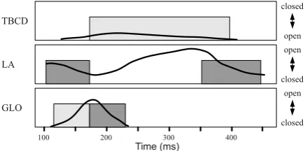
are associated with the onset, namely the shutting of GLO and of VEL, and the closure and release of LA. Similarly, the nucleus of the syllable consists of three goals, namely the relocation of TBCD and TBCL, and the opening of GLO. The presence and extent of these gestural goals are represented by filled rectangles in figure 1. Inter-gestural timings between these goals are specified relative to one another according to human data as described by Nam and Saltzman (2003).

TBCD

closed

open

GLO

open

closed

LA

open

closed

100 200 300 400

Time (ms)

Figure 1: Canonical examplepubfrom Saltzman

and Munhall (1989).

The presence of these discrete goals influences the vocal tract dynamically and continuously as modelled by the following non-homogeneous second-order linear differential equation:

Mz00+Bz0+K(z−z∗) =0. (1)

1_{Constrictionlocationsgenerally refer to the front-back}

dimension of the vocal tract and constrictiondegrees gener-ally refer to the top-down dimension.

Here,zis a continuous vector representing the

in-stantaneous positions of the nine tract variables,

z∗ is the target (equilibrium) positions of those

variables, and vectorsz0 andz00 represent the first

and second derivatives of z with respect to time

(i.e., velocity and acceleration), respectively. The

matrices M, B, and K are syllable-specific

coef-ficients describing the inertia, damping, and stiff-ness, respectively, of the virtual gestures. Gener-ally, this theory assumes that the tract variables are mutually independent, and that the system is criti-cally damped (i.e., the tract variables do not oscil-late around their equilibrium positions) (Nam and

Saltzman, 2003). The continuous state,z, of

equa-tion (1) is exemplified by black curves in figure 1.

2.2 Articulatory data

Tract variables provide the dimensions of an ab-stract gestural space independent of the physical characteristics of the speaker. In order to com-plete our articulatory model, however, we require physical data from which to infer these high-level articulatory goals.

Electromagnetic articulography (EMA) is a method to measure the motion of the vocal tract

during speech. In EMA, the speaker is placed

within a low-amplitude electromagnetic field pro-duced within a cube of a known geometry. Tiny sensors within this field induce small electric cur-rents whose energy allows the inference of artic-ulator positions and velocities to within 1 mm of error (Yunusova et al., 2009). We derive data for the following study from two EMA sources:

• The University of Edinburgh’s MOCHA

database, which provides

phonetically-balanced sentences repeated from TIMIT (Zue et al., 1989) uttered by a male and a female speaker (Wrench, 1999), and

• The University of Toronto’s TORGO

database, from which we select sentences repeated from TIMIT from two females and three males (Rudzicz et al., 2008). (Cerebrally palsied speech, which is the focus of this database, is not included here).

these onto the midsagittal plane. (Additionally, the MOCHA database provides velum (V) data on this plane, and TORGO provides the left and right lip corners (LL and RL) but these are excluded from study except where noted).

All articulatory data is aligned with its associ-ated acoustic data, which is transformed to Mel-frequency cepstral coefficients (MFCCs). Since the 2D EMA system in MOCHA and the 3D EMA system in TORGO differ in their recording rates, the length of each MFCC frame in each database must differ in order to properly align acoustics with articulation in time. Therefore, each MFCC frame covers 16 ms in the TORGO database, and 32 ms in MOCHA. Phoneme boundaries are de-termined automatically in the MOCHA database by forced alignment, and by a speech-language pathologist in the TORGO database.

We approximate the tract variable space from the physical space of the articulators, in general, through principal component analysis (PCA) on the latter, and subsequent sigmoid normalization

on[0,1]. For example, the LTH tract variable is

in-ferred by calculating the first principal component of the two-dimensional lower incisor (LI) motion in the midsagittal plane, and by normalizing the resulting univariate data through a scaled sigmoid. The VEL variable is inferred similarly from velum (V) EMA data. Tongue tip constriction location and degree (TTCL and TTCD, respectively) are

inferred from the 1stand 2ndprincipal components

of tongue tip (TT) EMA data, with TBCL and TBCD inferred similarly from tongue body (TB) data. Finally, the glottis (GLO) is inferred by voic-ing detection on acoustic energy below 150 Hz (O’Shaughnessy, 2000), lip aperture (LA) is the normalized Euclidean distance between the lips,

and lip protrusion (LP) is the normalized 2nd

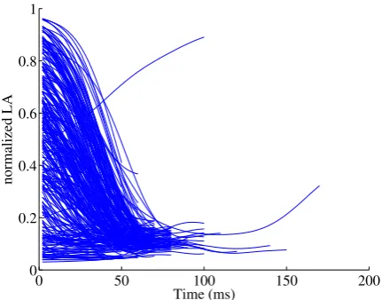
prin-cipal component of the midpoint between the lips. All PCA is performed without segmentation of the data. The result is a low-dimensional set of contin-uous curves describing goal-relevant articulatory variables. Figure 2, for example, shows the degree of the lip aperture (LA) over time for all instances

of the/b/phoneme in the MOCHA database. The

relevant articulatory goal of lip closure is evident.

3 Baseline systems

We now turn to the task of speech recognition. Traditional Bayesian learning is restricted to uni-versal or immutable relationships, and is

agnos-0 50 100 150 200

0 0.2 0.4 0.6 0.8 1

Time (ms)

normalized LA

Figure 2: Lip aperture (LA) over time during all

MOCHA instances of/b/.

tic towards dynamic systems or time-varying rela-tionships. Dynamic Bayes networks (DBNs) are directed acyclic graphs that generalize the power-ful stochastic mechanisms of Bayesian represen-tation to temporal sequences. We are free to ex-plicitly provide topological (i.e., dependency) re-lationships between relevant variables in our mod-els, which can include measurements of tract data.

We examine two baseline systems. The

first is the standard acoustic hidden Markov model (HMM) augmented with a bigram language

model, as shown in figure 3(a). Here,Wt →Wt+1

represents word transition probabilities, learned

by maximum likelihood estimation, and Pht →

Pht+1 represents phoneme transition probabilities

whose order is explicitly specified by the

relation-shipWt →Pht. Likewise, each phonemePh

con-ditions the sub-phoneme state, Qt, whose

transi-tion probabilitiesQt →Qt+1describe the

dynam-ics within phonemes. The variable Mt refers to

hidden Gaussian indices so that the likelihoods

of acoustic observations,Ot, are represented by a

mixture of 4, 8, 16, or 32 Gaussians for each state and each phoneme. See Murphy (2002) for a fur-ther description of this representation.

The second baseline model is the articulatory dynamic Bayes network (DBN-A). This augments the standard acoustic HMM by replacing hidden

indices, Mt, with discrete observations of the

vo-cal tract,Kt, as shown in figure 3(b). The pattern

of acoustics within each phoneme is dependent on a relatively restricted set of possible articulatory configurations (Roweis, 1999). To find these

de-scribe the articulatory data according to k-means clustering with the sum-of-squares error function.

During training, the DBN variable Kt is set

ex-plicitly to theindexof the mean vector nearest to

the current frame of EMA data at timet. In this

way, the relationship Kt →Ot allows us to learn

how discretized articulatory configurations affect acoustics. The training of DBNs involves a spe-cialized version of expectation-maximization, as described in the literature (Murphy, 2002;

Ghahra-mani, 1998). During inference, variablesWt,Pht,

and Kt become hidden and we marginalize over

their possible values when computing their likeli-hoods. Bigrams are computed by maximum like-lihood on lexical annotations in the training data.

M_t

O_t

M_t+1

O_t+1

Q_t

Ph_t

Q_t+1

Ph_t+1

W_t W_t+1

(a) HMM

K_t

O_t K_t+1

O_t+1 Q_t

Ph_t

Q_t+1 Ph_t+1 W_t W_t+1

(b) DBN-A

Figure 3: Baseline systems: (a) acoustic hidden Markov model and (b) articulatory dynamic Bayes

network. NodeWtrepresents the current word,Pht

is the current phoneme,Qt is that phoneme’s

dy-namic state, Ot is the acoustic observation,Mt is

the Gaussian mixture component, andKtis the

dis-cretized articulatory configuration. Filled nodes represent observed variables during training,

al-though only Ot is observed during recognition.

Square nodes are discrete variables while circular nodes are continuous variables.

4 Switching Kalman filter

Our first experimental system attempts speech recognition given only articulatory data. The true

state of the tract variables at timet−1 constitutes

a 9-dimensional vector, xt−1, of continuous

val-ues. Under the task dynamics model of section 2.1, the motions of these tract variables obey crit-ically damped second-order oscillatory relation-ships. We start with the simplifying assumption of linear dynamics here with allowances for random

Gaussianprocess noise, vt, since articulatory

be-haviour is non-deterministic. Moreover, we know that EMA recordings are subject to some error (usually less than 1 mm (Yunusova et al., 2009)),

so the actual observation at timet, yt, will not in

general be the true position of the articulators.

As-suming that the relationship betweenyt andxt is

also linear, and that the measurement noise, wt,

is also Gaussian, then the dynamical articulatory system can be described by

xt=Dtxt−1+vt

yt=Ctxt+wt.

(2)

Eqs. 2 form the basis of the Kalman filter which allows us to use EMA measurements di-rectly, rather than quantized abstractions thereof as in the DBN-A model. Obviously, since artic-ulatory dynamics vary significantly for different goals, we replicate eq. (2) for each phoneme and connect these continuous Kalman filters together with discrete conditioning variables for phoneme and word, resulting in the switching Kalman

fil-ter (SKF) model. Here, paramefil-tersDt andvt are

implicit in the relationshipxt →xt+1, and

param-eters Ct and wt are implicit in xt →yt. In this

model, observation yt is the instantaneous

mea-surements derived from EMA, andxt is their true

hidden states. These parameters are trained using expectation-maximization, as described in the lit-erature (Murphy, 1998; Deng et al., 2005).

5 Recognition with task dynamics

Our goal is to integrate task dynamics within an ASR system for continuous sentences called

TD-ASR. Our approach is to re-rank anN-best list of

sentence hypotheses according to a weighted like-lihood of their articulatory realizations. For

ex-ample, if a word sequenceWi :wi,1 wi,2 ... wi,m

has likelihoods LX(Wi) and LΛ(Wi) according to

purely acoustic and articulatory interpretations of an utterance, respectively, then its overall score would be

L(Wi) =αLX(Wi) + (1−α)LΛ(Wi) (3)

given a weighting parameterαset manually, as in

section 6.2. Acoustic likelihoodsLX(Wi) are

ob-tained from Viterbi paths through relevant HMMs in the standard fashion.

5.1 TheTADAcomponent

In order to obtain articulatory likelihoods,LΛ(Wi),

to task dynamics. To this end, we use

compo-nents from the open-source TADA system (Nam

and Goldstein, 2006), which is a complete imple-mentation of task dynamics. From this toolbox, we use the following components:

• A syllabic dictionary supplemented with

the International Speech Lexicon Dictionary (Hasegawa-Johnson and Fleck, 2007). This

breaks word sequences Wi into syllable

se-quencesSi consisting of onsets, nuclei, and

coda and covers all of MOCHA and TORGO.

• A syllable-to-gesture lookup table. Given

a syllabic sequence, Si, this table provides

the gestural goals necessary to produce those

syllables. For example, given the syllable

pub in figure 1, this table provides the

tar-gets for the GLO, VEL, TBCL, and TBCD tract variables, and the parameters for the

second-order differential equation, eq. 1,

that achieves those goals. These parameters have been empirically tuned by the authors

of TADA according to a generic,

speaker-independent representation of the vocal tract (Saltzman and Munhall, 1989).

• A component that produces the continuous

tract variable paths that produce an utter-ance. This component takes into account var-ious physiological aspects of human speech production, including intergestural and in-terarticulator co-ordination and timing (Nam and Saltzman, 2003; Goldstein and Fowler, 2003), and the neutral (“schwa”) forces of the vocal tract (Saltzman and Munhall, 1989). This component takes a sequence of gestu-ral goals predicted by the segment-to-gesture lookup table, and produces appropriate paths for each tract variable.

The result of the TADA component is a set of

N 9-dimensional articulatory paths, TVi,

neces-sary to produce the associated word sequences,Wi

for i=1..N. Since task dynamics is a

prescrip-tive model and fully deterministic,TVisequences

are the canonical or default articulatory

realiza-tions of the associated sentences. These canonical realizations are independent of our training data, so we transform them in order to more closely re-semble the observed articulatory behaviour in our EMA data. Towards this end, we train a switch-ing Kalman filter identical to that in section 4,

ex-cept the hidden state variablext is replaced by the

observed instantaneous canonical TVs predicted

by TADA. In this way we are explicitly learning

a relationship betweenTADA’s task dynamics and

human data. Since the lengths of these sequences are generally unequal, we align the articulatory

be-haviour predicted byTADAwith training data from

MOCHA and TORGO using standard dynamic time warping (Sakoe and Chiba, 1978). During

run-time, the articulatory sequenceyt most likely

to have been produced by the human data given the

canonical sequenceTVi is inferred by the Viterbi

algorithm through the SKF model with all other variables hidden. The result is a set of articulatory

sequences, TV∗i, for i=1..N, that represent the

predictions of task dynamics that better resemble our data.

5.2 Acoustic-articulatory inversion

In order to estimate the articulatory likelihood of an utterance, we need to evaluate each

trans-formed articulatory sequence,TV∗_i, within

proba-bility distributions ranging over all tract variables. These distributions can be inferred using acoustic-articulatory inversion. There are a number of ap-proaches to this task, including vector quantiza-tion, and expectation-maximization with Gaussian mixtures (Hogden and Valdez, 2001; Toda et al., 2008). These approaches accurately inferred the

xyposition of articulators to within 0.41 mm and

2.73 mm. Here, we modify the approach taken

by Richmond et al. (2003), who estimate proba-bility functions over the 2D midsagittal positions of 7 articulators, given acoustics, with a mixture-density network (MDN). An MDN is essentially a typical discriminative multi-layer neural network whose output consists of the parameters to Gaus-sian mixtures. Here, each GausGaus-sian mixture de-scribes a probability function over TV positions

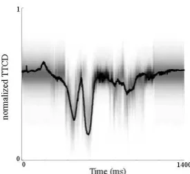
given the acoustic frame at time t. For

exam-ple, figure 4 shows an intensity map of the likely values for tongue-tip constriction degree (TTCD) for each frame of acoustics, superimposed with the ‘true’ trajectory of that TV. Our networks are trained with acoustic and EMA-derived data as de-scribed in section 2.2.

5.3 Recognition by reranking

During recognition of a test utterance, a standard acoustic HMM produces word sequence

hypothe-ses,Wi, and associated likelihoods,L(Wi), fori=

1..N. The expected canonical motion of the tract

Figure 4: Example probability density of tongue tip constriction degree over time, inferred from acoustics. The true trajectory is superimposed as a black curve.

for each of these word sequences and transformed by an SKF to better match speaker data, giving

TV∗i. The likelihoods of these paths are then

eval-uated within probability distributions produced by an MDN. The mechanism for producing the artic-ulatory likelihood is shown in figure 5. The overall likelihood, L(Wi) =αLX(Wi) + (1−α)LΛ(Wi), is

then used to produce a final hypothesis list for the given acoustic input.

6 Experiments

Experimental data is obtained from two sources,

as described in section 2.2. We procure 1200

sentences from Toronto’s TORGO database, and 896 from Edinburgh’s MOCHA. In total, there are 460 total unique sentence forms, 1092 total unique word forms, and 11065 total words uttered. Ex-cept where noted, all experiments randomly split the data into 90% training and 10% testing sets for 5-cross validation. MOCHA and TORGO data are never combined in a single training set due to dif-fering EMA recording rates. In all cases, models are database-dependent (i.e., all TORGO data is conflated, as is all of MOCHA).

For each of our baseline systems, we calcu-late the phoneme-error-rate (PER) and word-error-rate (WER) after training. The phoneme-error-rate is calculated according to the proportion of frames of speech incorrectly assigned to the proper

phoneme. The word-error-rate is calculated as

the sum of insertion, deletion, and substitution er-rors in the highest-ranked hypothesis divided by the total number of words in the correct orthogra-phy. The traditional HMM is compared by vary-ing the number of Gaussians used in the modellvary-ing

System Parameters PER (%) WER (%)

HMM

|M|=4 29.3 14.5

|M|=8 27.0 13.9

|M|=16 26.1 10.2

|M|=32 25.6 9.7

DBN-A

|K|=4 26.1 13.0

|K|=8 25.2 11.3

|K|=16 24.9 9.8

|K|=32 24.8 9.4

Table 1: Phoneme- and Word-Error-Rate (PER and WER) for different parameterizations of the baseline systems.

No. of Gaussians

1 2 3 4

LTH −0.28 −0.18 −0.15 −0.11

LA −0.36 −0.32 −0.30 −0.29

LP −0.46 −0.44 −0.43 −0.43

GLO −1.48 −1.30 −1.29 −1.25

TTCD −1.79 −1.60 −1.51 −1.47

TTCL −1.81 −1.62 −1.53 −1.49

TBCD −0.88 −0.79 −0.75 −0.72

TDCL −0.22 −0.20 −0.18 −0.17

Table 2: Average log likelihood of true tract vari-able positions in test data, under distributions pro-duced by mixture density networks with varying numbers of Gaussians.

of acoustic observations. Similarly, the DBN-A model is compared by varying the number of dis-crete quantizations of articulatory configurations, as described in section 3. Results are obtained by direct decoding. The average results across both databases, between which there are no significant

differences, are shown in table 1. In all cases

the DBN-A model outperforms the HMM, which highlights the benefit of explicitly conditioning acoustic observations on articulatory causes.

6.1 Efficacy of TD-ASR components

In order to evaluate the whole system, we start by evaluating its parts. First, we test how accurately the mixture-density network (MDN) estimates the position of the articulators given only information from the acoustics available during recognition. Table 2 shows the average log likelihood over each

tract variable across both databases. These

Acoustics

ASR

ASR

MDN

MDN W₁

W₂ ... W_N N-best hypotheses

TADA

TADA

TV₁ TV₂ ... TV_N Canonical

Tract Variables

TRANS

TRANS

TV*₁ TV*₂ ... TV*_N Modified

Tract Variables

P(TV_i*) _W* 1 W*₂ ... W*_N

Reranked list

Figure 5: The TD-ASR mechanism for deriving articulatory likelihoods,LΛ(Wi), for each word sequence

Wiproduced by standard acoustic techniques.

Manner Canonical Transformed

approximant 0.19 0.16

fricative 0.37 0.29

nasal* 0.24 0.18

retroflex 0.23 0.19

plosive 0.10 0.08

vowel 0.27 0.25

Table 3: Average difference between predicted

tract variables and observed data, on [0,1] scale.

(*) Nasals are evaluated only with MOCHA data, since TORGO data lacks velum measurements.

We evaluate how closely transformations to the

canonical tract variables predicted byTADAmatch

the data. Namely, we input the known orthography

for each test utterance intoTADA, obtain the

pre-dicted canonical tract variablesTV, and transform

these according to our trained SKF. The resulting predicted and transformed sequences are aligned with our measurements derived from EMA with dynamic time warping. Finally, we measure the average difference between the observed data and the predicted (canonical and transformed) tract variables. Table 3 shows these differences accord-ing to the phonological manner of articulation. In all cases the transformed tract variable motion is more accurate, and significantly so at the 95% con-fidence level for nasal and retroflex phonemes, and at 99% for fricatives. The practical utility of the transformation component is evaluated in its effect on recognition rates, as described below.

6.2 Recognition with TD-ASR

With the performance of the components of TD-ASR better understood, we combine these and study the resulting composite TD-ASR system.

0 0.2 0.4 0.6 0.8 1

8 8.5 9 9.5 10

α

WER (%)

TORGO MOCHA

Figure 6: Word-error-rate according to varyingα,

for both TORGO and MOCHA data.

Figure 6 shows the WER as a function ofαwith

TD-ASR andN=4 hypotheses per utterance. The

effect ofαis clearly non-monotonic, with

articula-tory information clearly proving useful. Although systems whose rankings are weighted solely by the articulatory component perform better than the ex-clusively acoustic systems, the lists available to the former are procured from standard acoustic ASR. Interestingly, the gap between systems trained to

the two databases increases as αapproaches 1.0.

Although this gap is not significant, it may be the result of increased inter-speaker articulatory varia-tion in the TORGO database, which includes more than twice as many speakers as MOCHA.

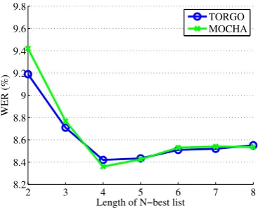
Figure 7 shows the WER obtained with

TD-ASR given varying-length N-best lists and α =

0.7. TD-ASR accuracy at N=4 is significantly

better than both TD-ASR atN=2 and the

base-line approaches of table 1 at the 95% confidence

level. However, for N >4 there is a noticeable

2 3 4 5 6 7 8 8.2

8.4 8.6 8.8 9 9.2 9.4 9.6 9.8

Length of N−best list

WER (%)

TORGO MOCHA

Figure 7: Word-error-rate according to

vary-ing lengths of N-best hypotheses used, for both

TORGO and MOCHA data.

The optimal parameterization of the TD-ASR model results in an average word-error-rate of

8.43%, which represents a 10.3% relative error

re-duction over the best parameterization of our base-line models. The SKF model of section 4 differs from the HMM and DBN-A baseline models only in its use of continuous (rather than discrete) hid-den dynamics and in its articulatory observations. However, its performance is far more variable, and

less conclusive. On the MOCHA database the

SKF model had an average of 9.54% WER with

a standard deviation of 0.73 over 5 trials, and an

average of 9.04% WER with a standard deviation

of 0.64 over 5 trials on the TORGO database.

De-spite the presupposed utility of direct articulatory observations, the SKF system does not perform significantly better than the best DBN-A model.

Finally, the experiments of tables 6 and 7 are repeated with the canonical tract variables passed untransformed to the probability maps generated by the MDNs. Predictably, resulting articulatory

likelihoodsL_Λare less representative and

increas-ing their contributionα to the hypothesis

rerank-ing does not improve TD-ASR performance sig-nificantly, and in some instances worsens it.

Al-though TADA is a useful prescriptive model of

generic articulation, its use must be tempered with knowledge of inter-speaker variability.

7 Discussion and conclusions

The articulatory medium of speech rarely informs

modern speech recognition. We have

demon-strated that the use of direct articulatory knowl-edge can substantially reduce phoneme and word

errors in speech recognition, especially if that knowledge is motivated by high-level abstrac-tions of vocal tract behaviour. Task dynamic the-ory provides a coherent and biologically plausible model of speech production with consequences for phonology (Browman and Goldstein, 1986), neu-rolinguistics (Guenther and Perkell, 2004), and the evolution of speech and language (Goldstein et al., 2006). We have shown that it is also useful within speech recognition.

We have overcome a conceptual impediment in integrating task dynamics and ASR, which is the former’s deterministic nature. This integration is accomplished by stochastically transforming pre-dicted articulatory dynamics and by calculating the likelihoods of these dynamics according to speaker data. However, there are several new av-enues for exploration. For example, task dynamics lends itself to more general applications of con-trol theory, including automated self-correction, rhythm, co-ordination, and segmentation (Fried-land, 2005). Other high-level questions also re-main, such as whether discrete gestures are the correct biological and practical paradigm, whether a purely continuous representation would be more appropriate, and whether this approach general-izes to other languages.

In general, our experiments have revealed very little difference between the use of MOCHA and

TORGO EMA data. Anad hocanalysis of some

of the errors produced by the TD-ASR system found no particular difference between how sys-tems trained to each of these databases recognized nasal phonemes, although only those trained with MOCHA considered velum motion. Other errors common to both sources of data include phoneme insertion errors, normally vowels, which appear to co-occur with some spurious motion of the tongue

between segments, especially for longer N-best

lists. Despite the relative slow motion of the ar-ticulators relative to acoustics, there remains some intermittent noise.

As more articulatory data becomes available and as theories of speech production become more refined, we expect that their combined value to speech recognition will become indispensable.

Acknowledgments

References

Catherine P. Browman and Louis M. Goldstein. 1986. To-wards an articulatory phonology. Phonology Yearbook, 3:219–252.

Alessandro D’Ausilio, Friedemann Pulvermuller, Paola Salmas, Ilaria Bufalari, Chiara Begliomini, and Luciano Fadiga. 2009. The motor somatotopy of speech percep-tion.Current Biology, 19(5):381–385, February. Jianping Deng, M. Bouchard, and Tet Yeap. 2005. Speech

Enhancement Using a Switching Kalman Filter with a Per-ceptual Post-Filter. InAcoustics, Speech, and Signal Pro-cessing, 2005. Proceedings. (ICASSP ’05). IEEE Interna-tional Conference on, volume 1, pages 1121–1124, 18-23,. Bernard Friedland. 2005. Control System Design: An

Intro-duction to State-Space Methods. Dover.

Zoubin Ghahramani. 1998. Learning dynamic Bayesian net-works. In Adaptive Processing of Sequences and Data Structures, pages 168–197. Springer-Verlag.

Louis M. Goldstein and Carol Fowler. 2003. Articulatory phonology: a phonology for public language use. Phonet-ics and Phonology in Language Comprehension and Pro-duction: Differences and Similarities.

Louis Goldstein, Dani Byrd, and Elliot Saltzman. 2006. The role of vocal tract gestural action units in understanding the evolution of phonology. In M.A. Arib, editor,Action to Language via the Mirror Neuron System, pages 215– 249. Cambridge University Press, Cambridge, UK. Frank H. Guenther and Joseph S. Perkell. 2004. A

neu-ral model of speech production and its application to studies of the role of auditory feedback in speech. In Ben Maassen, Raymond Kent, Herman Peters, Pascal Van Lieshout, and Wouter Hulstijn, editors, Speech Motor Control in Normal and Disordered Speech, chapter 4, pages 29–49. Oxford University Press, Oxford.

William J. Hardcastle and Nigel Hewlett, editors. 1999.

Coarticulation – Theory, Data, and Techniques. Cam-bridge University Press.

Mark Hasegawa-Johnson and Margaret Fleck. 2007. Inter-national Speech Lexicon Project.

John Hogden and Patrick Valdez. 2001. A stochastic articulatory-to-acoustic mapping as a basis for speech recognition. InProceedings of the 18th IEEE Instrumen-tation and Measurement Technology Conference, 2001. IMTC 2001, volume 2, pages 1105–1110 vol.2.

Katrin Kirchhoff. 1999. Robust Speech Recognition Us-ing Articulatory Information. Ph.D. thesis, University of Bielefeld, Germany, July.

Alvin M. Liberman and Ignatius G. Mattingly. 1985. The motor theory of speech perception revised. Cognition, 21:1–36.

Konstantin Markov, Jianwu Dang, and Satoshi Nakamura. 2006. Integration of articulatory and spectrum features based on the hybrid HMM/BN modeling framework.

Speech Communication, 48(2):161–175, February. Kevin Patrick Murphy. 1998. Switching Kalman Filters.

Technical report.

Kevin Patrick Murphy. 2002. Dynamic Bayesian Networks: Representation, Inference and Learning. Ph.D. thesis, University of California at Berkeley.

Hosung Nam and Louis Goldstein. 2006. TADA (TAsk Dy-namics Application) manual.

Hosung Nam and Elliot Saltzman. 2003. A competitive, cou-pled oscillator model of syllable structure. InProceedings of the 15th International Congress of Phonetic Sciences (ICPhS 2003), pages 2253–2256, Barcelona, Spain. Douglas O’Shaughnessy. 2000. Speech Communications –

Human and Machine. IEEE Press, New York, NY, USA. Korin Richmond, Simon King, and Paul Taylor. 2003.

Modelling the uncertainty in recovering articulation from acoustics.Computer Speech and Language, 17:153–172. Sam T. Roweis. 1999. Data Driven Production Models for

Speech Processing. Ph.D. thesis, California Institute of Technology, Pasadena, California.

Frank Rudzicz, Pascal van Lieshout, Graeme Hirst, Gerald Penn, Fraser Shein, and Talya Wolff. 2008. Towards a comparative database of dysarthric articulation. In Pro-ceedings of the eighth International Seminar on Speech Production (ISSP’08), Strasbourg France, December. Frank Rudzicz. 2009. Applying discretized articulatory

knowledge to dysarthric speech. In Proceedings of the 2009 IEEE International Conference on Acoustics, Speech, and Signal Processing (ICASSP09), Taipei, Tai-wan, April.

Hiroaki Sakoe and Seibi Chiba. 1978. Dynamic program-ming algorithm optimization for spoken word recognition.

IEEE Transactions on Acoustics, Speech, and Signal Pro-cessing, ASSP-26, February.

Elliot L. Saltzman and Kevin G. Munhall. 1989. A dynam-ical approach to gestural patterning in speech production.

Ecological Psychology, 1(4):333–382.

Elliot M. Saltzman, 1986.Task dynamic co-ordination of the speech articulators: a preliminary model, pages 129–144. Springer-Verlag.

Tomoki Toda, Alan W. Black, and Keiichi Tokuda. 2008. Statistical mapping between articulatory movements and acoustic spectrum using a Gaussian mixture model.

Speech Communication, 50(3):215–227, March.

Alan Wrench. 1999. The MOCHA-TIMIT articulatory database, November.

Yana Yunusova, Jordan R. Green, and Antje Mefferd. 2009. Accuracy Assessment for AG500, Electromagnetic Artic-ulograph. Journal of Speech, Language, and Hearing Re-search, 52:547–555, April.

Victor Zue, Stephanie Seneff, and James Glass. 1989. Speech Database Development: TIMIT and Beyond. In