Munich Personal RePEc Archive
Catch-Up: A Rule That Makes Service
Sports More Competitive
Brams, Steven J. and Ismail, Mehmet S. and Kilgour, D.
Marc and Stromquist, Walter
19 December 2016
Catch-Up: A Rule That Makes Service Sports More
Competitive
∗
Steven J. Brams
Department of Politics, New York University, New York, NY 10012, USA
steven.brams@nyu.edu
Mehmet S. Ismail
Department of Political Economy, King’s College London, London, WC2R 2LS, UK
mehmet.s.ismail@gmail.com
D. Marc Kilgour
Department of Mathematics, Wilfrid Laurier University, Waterloo, Ontario N2L 3C5, Canada
mkilgour@wlu.ca
Walter Stromquist
132 Bodine Road, Berwyn, PA 19312, USA
mail@walterstromquist.com
February 2018
Abstract
Service sports include two-player contests such as volleyball, badminton, and squash. We analyze four rules, including the Standard Rule (SR), in which a player continues to serve until he or she loses. The Catch-Up Rule (CR) gives the serve to the player who has lost the previous point—as opposed to the player who won the previous point, as underSR. We also consider two Trailing Rules that make the server the player who trails in total score. Surprisingly, compared with SR, only
CR gives the players the same probability of winning a game while increasing its expected length, thereby making it more competitive and exciting to watch. Unlike one of the Trailing Rules, CR is strategy-proof. By contrast, the rules of tennis fix who serves and when; its tiebreaker, however, keeps play competitive by being fair—not favoring either the player who serves first or who serves second.
1
Introduction
In service sports, competition between two players (or teams) involves one player serving some object—usually a ball, but a “shuttlecock” in badminton—which the opponent tries to return. Service sports include tennis, table tennis (ping pong), racquetball, squash, badminton, and volleyball.
If the server is successful, he or she wins the point; otherwise—in most, but not all, of these sports—the opponent does. If the competitors are equally skilled, the server generally has a higher probability of winning than the receiver. We will say more later about what constitutes winning in various service sports.
In some service sports, such as tennis and table tennis, the serving order is fixed—the rules specify when and for how long each player serves. By contrast, the serving order in most service sports, including racquetball, squash, badminton, and volleyball, is variable: It depends on who won the last point.1
In these sports, if the server won the last point, then he or she serves on the next point also, whereas if the receiver won, he or she becomes the new server. In short, the winner of the last point is the next server. We call this the Standard Rule (SR).
In this paper, we analyze three alternatives to SR, all of which are variable. The simplest is the
• Catch-Up Rule (CR): Server is the loser of the previous point—instead of the winner, as under SR.2
The two other serving rules are Trailing Rules (TRs), which we also consider variable: A player who is behind in points becomes the server. Thus, these rules take into account the entire history of play, not just who won or lost the previous point. If there is a tie, then who becomes the server depends on the situation immediately prior to the tie:
• TRa: Server is the player who was ahead in points prior to the tie;
• TRb: Server is the player who was behind in points prior to the tie.
We calculate the players’ win probabilities under all four rules. Our only data about the players are their probabilities of winning a point on serve, which we take to be equal exactly when the players are equally skilled. We always assume that all points (rounds) are independent. Among other findings, we prove that SR, CR, and TRa are strategy-proof (or incentive compatible)—neither the server nor the receiver can ever benefit from deliberately losing a point. But TRb is strategy-vulnerable: UnderTRb, it is possible for
1
In game theory, a game is defined by “the totality of the rules that describe it” [14, p. 49]. The main difference between fixed-order and variable-order serving rules is that when the serving order is variable, the course of play (order of service) may depend on the results on earlier points, whereas when the order is fixed, then so is the course of play. Put another way, the serving order is determined exogenously in fixed-order sports but endogenously in variable-order sports.
2
The idea of catch-up is incorporated in the game of Catch-Up (see
a player to increase his or her probability of winning a game by losing a point deliberately, under certain conditions that we will spell out.
We analyze the probability that each player wins a game by being the first to score a certain number of points (Win-by-One); later, we analyze Win-by-Two, in which the winner is the first player to score at least the requisite number of points and also to be ahead by at least two points at that time. We also assess the effects of the different rules on the expected length of a game, measured by the total number of points until some player wins.
Most service sports, whether they use fixed or variable serving rules, use Win-by-Two. We compare games with and without Win-by-Two to assess the effects of this rule. Although Win-by-Two may prolong a game, it has no substantial effect on the probability of a player’s winning if the number of points needed to win is sufficiently large and the players are equally skilled. The main effect of Win-by-Two is to increase the drama and tension of a close game.
The three new serving rules give a break to a player who loses a point, or falls behind, in a game. This change can be expected to make games, especially games between equally skilled players, more competitive—they are more likely to stay close to the end and, hence, to be more exciting to watch.
CR, like SR, is Markovian in basing the serving order only on the outcome of the previous point, whereas TRa and TRb take accumulated scores into account.3
The two
TRs may give an extra advantage to weaker players, which is not true of CR. As we will show, under Win-by-One,CR gives the players exactly the same probabilities of winning a game as SR does. At the same time, CR increases the expected length of games and, therefore, also their competitiveness. For this reason, our major recommendation is that
CR replaceSR to enhance competition in service sports with variable service rules.
2
Win-by-One
2.1
Probability of Winning
Assume thatAhas probability pof winning a point whenAserves, and B has probability
q of winning a point when B serves. (Warning! In this paper, q is not an abbreviation for 1−p.) We always assume that A serves first, and that 0< p <1 and 0< q <1. We will use pronouns “he” for A, “she” forB.
We begin with the simple case of Best-of-3, in which the first player to reach 2 points wins. There are three ways for A to win: (1) by winning the first two points (which we denote AA), (2) by winning the first and third points (ABA), and (3) by winning the second and third points (BAA).
3
Any of these “win sequences” can occur under any of the four rules described in the Introduction (SR, CR, TRa, TRb), but each rule would imply a different sequence of servers. A win sequence tells us which player won each point, but it does not tell us which player served each point. For this purpose we define an “outcome” as a win sequence that includes additional information: We use A or B when either player wins when serving, and A and B when either player wins when the other player is serving. Thus, a bar over a letter marks a server loss.
For example, under SR, the win sequence AA occurs when A wins two serves in a row, and so the outcome is AA (no server losses). The win sequence ABA occurs when
A serves the first point and wins, A retains the serve for the second point and loses, and thenB gains the serve for the third point and loses, giving the outcomeABA(two server losses). Under SR the win sequence BAA corresponds to the outcome BAA.
Because we assume that serves are independent events—in particular, not dependent on the score at any point—we can calculate the probability of an outcome by multiplying the appropriate probabilities serve by serve. For example, the outcome AA occurs with probability p2
, because it requires two server wins by A. The outcome ABA has prob-ability p(1−p)(1−q), and the outcome BAA has probability (1−p)(1−q)p. Adding these three probabilities gives the total probability thatA wins Best-of-3 under SR:
P rSR(A) = p
2
+p(1−p)(1−q) + (1−p)(1−q)p= 2p−p2 −2pq+ 2p2q.
The translation from outcome to probability is direct: A, B, A, B correspond to probabilities p, q, (1−q), (1−p), respectively, whatever the rule. Under CR, the win sequences AA, ABA, BAAcorrespond to the outcomes AA (probability p(1−q)),ABA
(probability pqp) and BAA(probability (1−p)p(1−q)) respectively. So the probability that A wins Best-of-3 under CR is
P rCR(A) =p(1−q) +pqp+ (1−p)p(1−q) = 2p−p
2
−2pq+ 2p2
q.
Thus, the totals for SR and CR are the same, even though the probabilities being added are different.
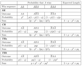
Table 1 extends this calculation to TRa and TRb. It shows that A has the same probability of winning when using SR, CR, and TRa, but a different probability when using TRb. The latter probability is generally smaller:
P rSR(A) = P rCR(A) =P rT Ra(A)≥P rT Rb(A),
with equality only whenp+q = 1. The intuition behind this result is thatTRb most helps the player who falls behind. This player is likely to be B when Aserves first, making B’s probability of winning greater, and A’s less, than under the other rules. (Realistically, serving is more advantageous than receiving in most service sports, though volleyball is an exception, as we discuss later.)
Probability thatAwins Expected Length
Win sequence: AA ABA BAA
SR
Outcome AA ABA BAA
Probability p2 p(1−p)(1−q) (1−p)(1−q)p
Sum 2p−p2−2pq+ 2p2q 3−q−p2+pq
CR
Outcome AA ABA BAA
Probability p(1−q) pqp (1−p)p(1−q)
Sum 2p−p2−2pq+ 2p2q 2 +p−p2+pq
TRa
Outcome AA ABA BAA
Probability p(1−q) pqp (1−p)p(1−q)
Sum 2p−p2−2pq+ 2p2q 2 +p−p2+pq
TRb
Outcome AA ABA BAA
Probability p(1−q) pq(1−q) (1−p)p2
[image:7.612.129.481.75.357.2]Sum p+p2−p3−pq2 2 +p−p2+pq
Table 1: Probability that A wins and Expected Length for a Best-of-3 game
and tedious. Instead of three possible ways in which each player can win, there are ten. We carried out these calculations and found that
P rSR(A) =P rCR(A)≥P rT Ra(A),
with equality only in the case ofp+q = 1. When the players are of equal strength (p=q) we also haveP rT Ra(A)≥P rT Rb(A),with equality only whenp= 1/2. But in the
Best-of-5 case, whenp6=q, no inequality holds generally. We can even haveP rT Rb(A)> P rSR(A)
for certain values of pand q.
But does the equality of A’s winning under SR and CR hold generally? Theorem 1 below shows that this is indeed the case.
Theorem 1. Let k ≥1. In a Best-of-(2k+ 1) game, P rSR(A) = P rCR(A).
For a proof, see the Appendix. Kingston [9] proved that, in a Best-of-(2k+ 1) game with k ≥ 1, the probability of A’s winning under SR is equal to the probability of A’s winning under any fixed rule that assignsk+ 1 serves to A, andk serves toB; this proof was simplified, and made more intuitive, by Anderson [2]. We extend their proof to the case ofCR and even more generally to the case in which a player’s probability of winning a point when he or she serves is variable.4
4
The basis of the proof is the idea of serving schedule, which is a record of server wins and server losses organized according to the server. The schedule lists the results of k1 serves by A, and then k serves by B. To illustrate, the description of a Best-of-3
game requires a server schedule of length 3, consisting of a record of whether the server won or lost on A’s first and second serves, and on B’s first serve. The serving schedule (W, L, L), for instance, records that A1 =W (i.e., A won on his first serve), A2 = L (A
lost on his second serve), and B1 =L (B lost on her first serve). The idea is that, if the
serving schedule is fixed, then both serving rules, SR and CR, give the same outcome as an Auxiliary Rule (AR), in which A serves twice and thenB serves once. Specifically,
• AR: (A1 =W, A2 =L, B1 =L), outcomeABA. A wins 2-1. • SR: (A1 =W, A2 =L, B1 =L), outcome ABA. A wins 2-1. • CR: (A1 =W, B1 =L), outcome AA. A wins 2-0.
Observe that the winner is the same under each rule, despite the differences in outcomes and scores. The basis of our proof is a demonstration that, if the serving schedule is fixed, then the winners under AR, SR, and CR are identical.
The AR service rule is particularly simple and permits us to establish a formula to determine win probabilities. The fact that the AR,SR, and CR service rules have equal win probabilities makes this representation more useful.
Corollary 1. The probability that Awins a Best-of-(2k+1)game under any of the service rules SR, CR, or AR is
P rAR(A) = P rSR(A) = P rCR(A)
=
k+1
X
n=1
n−1
X
m=0
pn(1−p)k+1−n
qm(1−q)k−m
k+ 1
n
k m
.
Proof. As shown in the proof of Theorem 1, each of these probabilities is equal to the probability of choosing a service schedule in whichAhas at leastk+1 total wins. Suppose that A has exactly n server wins among his k+1 serves. If n= 0, A must lose under any of the rules. If n= 1,2, . . . , k+ 1, thenA wins if and only if B has m server wins among her firstk serves, with m≤n−1. The probability above follows directly.
2.2
Expected Length of a Game
The different service rules may affect not only the probability of A’s winning but also the expected length (EL) of a game. To illustrate the latter calculation, consider SR for
of her serves with the same probability q. But what if A wins his ith serve with probability pi, for
i = 1,2, . . ., and that B wins her jth serve with probability qj, for j = 1,2, . . .? Then, the proof of
Theorem 1 still applies. We can even make A’s probability pi depend on the results of A’s previous
Best-of-3 in the case p = q. Clearly, the game lasts either two or three serves. Table 1 shows that Awill win with probabilityp2
after 2 serves; also, B will win with probability
p(1−p) after 2 serves. Therefore, the probability that the game ends after two serves is
p2
+p(1−p) =p, so the probability that it ends after three serves is (1−p). Hence, the expected length is
ELSR = 2p+ 3(1−p) = 3−p.
To illustrate, if p = 0, servers always lose, so the game will take 3 serves—and 2 switches of server—before the player who starts (A) loses 2 points to 1. On the other hand, if p= 1, ELSR = 2, because A will win on his first two serves.
By a similar calculation,ELCR = 2 +p. We also give results for the twoTRs in Table
1, producing the following ranking of expected lengths for Best-of-3 games if p > 1 2,
ELT Rb =ELT Ra=ELCR > ELSR.
Observe that the expected length of a game for Best-of-3 is a minimum underSR. To give an intuition for this conclusion, if A is successful on his first serve, he can end play with a second successful serve, which is fairly likely if p is large. On the other hand, CR and the TRs shift the service to the other player, who now has a good chance of evening the score if p > 1
2.
Calculations for Best-of-5 games show that
ELT Rb =ELT Ra> ELCR > ELSR.
Thus, both TRs have a greater expected length than CR, and the length of CR in turn exceeds the length of SR.5
Theorem 2. In a Best-of-(2k+ 1) game for any k ≥ 1 and 0 < p < 1, 0 < q < 1, the expected length of a game is greater under CR than under SR if and only if p+q >1.
The proof of Theorem 2 appears in the Appendix. The proof involves a long string of sums that we were unable to simplify or evaluate. However, we were able to manipulate them enough to prove the theorem. A more insightful proof would be welcome.
Henceforth, we focus on the comparison between SR and CR for two reasons:
1. UnderCR, the probability of a player’s winning is the same as under SR (Theorem 1).
2. Under CR, the length of the game is greater (in expectation) than under SR, pro-vided p+q >1 (Theorem 2).
For these reasons, we believe that most service sports currently using the SR rule would benefit from the CR rule. Changes should not introduce radical shifts, such as changing the probability of winning. At the same time, CR would make play appear to be more
5
competitive and, therefore, more likely to stimulate fan (and player) interest. CR satisfies both of our criteria.
CR keeps games close by giving a player who loses a point the opportunity to serve and, therefore, to catch up, given p+q >1. Consequently, the expected length of games will, on average, be greater under CR than SR. For Best-of-3 games, if p = q = 2
3, then
ELCR = 83, whereasELSR = 7
3. Still, the probability thatAwins is the same under both
rules (16
27 = 0.592, from Table 1). By Theorem 1, each player can rest assured that CR,
compared with SR, does not affect his or her chances of winning. It is true under SR and CR that if p = 2
3, then A has almost a 3:2 advantage in
probability of winning (16
27 = 0.592) in Best-of-3. But this is less than the 2:1 advantageA
would enjoy if a game were decided by just one serve. Furthermore, A’s advantage drops ask increases for Best-of-(2k+ 1), so games that require more points to win tend to level the playing field. In Best-of-5, A’s winning probability drops to 0.568.
Because the two TRs do even better than CR in lengthening games, would not one be preferable in making games closer and more competitive? The answer is “yes,” but they would reduce P r(A), relative to SR (and CR), and so would be a more significant departure from the present rule. For Best-of-3, P rT Rb(A) = 1427 = 0.519, which is 12.5%
lower than P rSR(A) = P rCR(A) =
16
27 = 0.592. 6
But TRb has a major strike against it that the other rules do not, which we explore next.
2.3
Incentive Compatibility
As discussed in the Introduction, a rule is strategy-proof or incentive compatible if no player can ever benefit from deliberately losing a point; otherwise, it isstrategy-vulnerable.7
Theorem 3. TRb is strategy-vulnerable, whereas SR and CR are strategy-proof. TRa is strategy-proof whenever p+q >1.
Proof. To show that TRb is strategy-vulnerable, assume a Best-of-3 game played under
TRb. We will show that there are values ofpandqsuch thatAcan increase his probability of winning the game by deliberately losing the first point.
Recall that A serves first. If A loses on the initial serve, the score is 0-1, so under
TRb,A serves again. If he wins the second point (with probabilityp), he ties the score at 1-1 and serves once more, again winning with probability p. Thus, by losing deliberately,
A wins the game with probability p2
.
If A does not deliberately lose his first serve, then there are three outcomes in which he will win the game:
6
We recognize that it may be desirable to eliminate entirely the first-server advantage, but this is difficult to accomplish in a service sport, as the ball must be put into play somehow. In fact, the first-server advantage decreases as the number of points required to win increases. Of course, any game is ex-ante fair if the first server is chosen randomly according to a coin toss, but it would be desirable to align ex-ante and ex-post fairness. As we show later, the serving rules of the tiebreaker in tennis achieve this alignment exactly
7
• AA with probability p(1−q)
• ABAwith probability pq(1−q)
• BAAwith probability (1−p)p2
.
Therefore, A’s probability of winning the game is greater when A deliberately loses the first serve if and only if
p2
>(p−pq) + (pq−pq2
) + (p2 −p3
),
which is equivalent to p(1−p2 −q2
)<0. Because p >0, it follows that Amaximizes the probability that he wins the game by deliberately losing his first serve when
p2+q2 >1.
In (p, q)-space, this inequality describes the exterior of a circle of radius 1 centered at (p, q) = (0,0). Because the probabilities p and q can be any numbers within the unit square of this space, it is possible that (p, q) lies outside this circle. If so,A’s best strategy is to deliberately lose his initial serve.
We next show that SRis strategy-proof. In a Best-of-(2k+ 1) game played underSR, let (C, x, y) denote a state in which playerC(C =A orB) is the server,A’s score isx, and
B’s isy. For example, when the game starts, the state is (A,0,0). LetWAS(C, x, y) denote A’s win probability from state (C, x, y) under SR. It is clear that A’s win probability
WAS(A, x, y) is increasing in x.
To show that a game played under SR is strategy-proof for A, we must show that
WAS(A, x+ 1, y)≥WAS(B, x, y+ 1) for any xand y. Now
WAS(A, x, y) =pWAS(A, x+ 1, y) + (1−p)WAS(B, x, y+ 1),
which implies that
p[WAS(A, x+ 1, y)−WAS(A, x, y)]
+ (1−p)[WAS(B, x, y+ 1)−WAS(A, x, y)] = 0.
Because 0< p <1 andWAS(A, x+ 1, y)≥WAS(A, x, y), the first term is nonnegative, so
the second must be nonpositive. It follows that
WAS(B, x, y+ 1) ≤WAS(A, x, y)≤WAS(A, x+ 1, y),
as required. Thus, A cannot gain under SR by deliberately losing a serve, so SR is strategy-proof for A. By an analogous argument, SR is also strategy-proof for B.
We next show that CR is strategy-proof. We use the same notation for states, and denoteA’s win probability from state (C, x, y) byWAC(C, x, y) andB’s byWBC(C, x, y).
To show that a game played under CR is strategy-proof for A, we must show that
WAC(B, x+ 1, y)≥WAC(A, x, y + 1) for any xand y. Now
WAC(A, x, y) =pWAC(B, x+ 1, y) + (1−p)WAC(A, x, y+ 1),
which implies that
p[WAC(B, x+ 1, y)−WAC(A, x, y)]
+ (1−p) [WAC(A, x, y+ 1)−WAC(A, x, y)] = 0.
Again, it follows that
WAC(A, x, y+ 1)≤WAC(A, x, y)≤WAC(B, x+ 1, y),
as required. Thus a game played under CR is strategy-proof for A, and by analogy it is strategy-proof for B.
The proof that TRa is strategy-proof is left for the Appendix.
To illustrate the difference between TRa and TRb and indicate its implications for strategy-proofness, suppose that the score is tied and that A has the serve. If A delib-erately loses, B will be ahead by one point, so A will serve the second point. If A is successful, the score is again tied, and TRb awards the next serve to A, whereas TRa
gives it to B, who was ahead prior to the most recent tie. If p >1−q, the extra serve is an advantage to A.
Suppose that the players are equally skilled at serving (p =q) in the Best-of-3 coun-terexample establishing that TRb is not strategy-proof. Then the condition for deliber-ately losing to be advantageous under TRb is p > 0.707. Thus, strategy-vulnerability arises in this simple game if both players have a server win probability greater than about 0.71, which is high but not unrealistic in most service sports.
From numerical calculations, we know that for Best-of-5 (and longer) games, neither
TRa (nor the strategy-vulnerableTRb) has the same win probability forAasSR, whereas by Theorem 1 CR maintains it in Win-by-One games of any length. This seems a good reason for focusing on CR as the most viable alternative to SR, especially because our calculations show that CR increases the expected length of Best-of-5 and longer games, thereby making them appear more competitive.
Most service sports are not Win-by-One but Win-by-Two (racquetball is an exception, discussed in Section 3). Ifk+ 1 points are required to win, and if the two players tie atk
points, then one player must outscore his or her opponent by two points in a tiebreaker in order to win.
We next analyze Win-by-Two’s effect on A’s probability of winning and the expected length of a game.8
We note that the service rule, which we take to beSR orCR, affects
8
the tiebreak; starting in a tied position,SR gives one player the chance of winning on two consecutive serves, whereas underCR a player who loses a tiebreak must lose at least once on serve. We later consider sports with fixed rules for serving and ask how Win-by-Two affects them.
3
Win-by-Two
To illustrate Win-by-Two, consider Best-of-3, in which a player wins by being the first to receive 2 points and by achieving at least two more points than the opponent. In other words, 2-0 is winning but 2-1 is not; if a 1-1 tie occurs, the winner will be the first player to lead by 2 points and will thus require more than 3 points.
3.1
Standard Rule Tiebreaker
Consider the ways in which a 1-1 tie can occur under SR. There are two sequences that produce such a tie:
• AB with probability p(1−p)
• BA with probability (1−p)(1−q).
Thus, the probability of a 1-1 tie is
(p−p2
) + (1−p−q+pq) = 1 +pq−p2 −q,
or 1−p if p = q. As p approaches 1 (and p= q), the probability of a tie approaches 0, whereas if p= 2
3, the probability is 1 3.
We now assume that p = q (as we will do for the rest of the paper). In a Best-of-(2k+ 1) tiebreaker played under SR, recall that P rSR(A) is the probability thatA wins
when he serves first. Then 1−P rSR(A) is the probability that B wins when A serves
first. Sincep=q, 1−P rSR(A) is also the probability that Awins the tiebreaker when B
serves first. Then it follows that P rSR(A) must satisfy the following recursion:
P rSR(A) =p
2
+ [p(1−p)(1−P rSR(A))] + [(1−p)
2
P rSR(A)].
The first term on the right-hand side gives the probability that A wins the first two points. The second term gives the probability of sequence AB—so A wins initially and then loses, recreating a tie—times the probability that A wins whenB serves first in the next tiebreaker. The third term gives the probability of sequence BA—in whichA loses
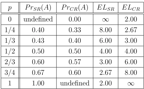
p P rSR(A) P rCR(A) ELSR ELCR
[image:14.612.183.424.76.224.2]0 undefined 0.00 ∞ 2.00 1/4 0.40 0.33 8.00 2.67 1/3 0.43 0.40 6.00 3.00 1/2 0.50 0.50 4.00 4.00 2/3 0.60 0.57 3.00 6.00 3/4 0.67 0.60 2.67 8.00 1 1.00 undefined 2.00 ∞
Table 2: Probability (P r) that A wins, and Expected Length of a Game (EL), under SR
and CR for various values of p.
initially and then B loses, recreating a tie—times the probability that A wins the next tiebreaker. Because p >0, this equation can be solved for P rSR(A) to yield
P rSR(A) =
1 3−2p.
Table 2 presents the probabilities and expected lengths underSRand CR correspond-ing to various values of p. Under SR, observe that A’s probability of winning is greater than p when p = 1
3 and less when p = 2
3. More generally, it is easy to show that
P rSR(A) > p if 0 < p < 21, and P rSR(A) < p if 1
2 < p < 1. Thus, A does worse in a
tiebreaker than if a single serve decides a tied game when 1
2 < p <1. Whenp= 1, A will
win the tiebreaker with certainty, because he serves first and will win every point. At the other extreme, whenp approaches 0, P rSR(A) approaches 13.
When there is a tie just before the end of a game, Win-by-Two not only prolongs the game over Win-by-One but also changes the players’ win probabilities. If p = 2
3,
under Win-by-One, sequence AB has twice the probability of producing a tie as BA. Consequently,Bhas twice the probability of serving the tie-breaking point (and, therefore, winning) than A does under Win-by-One.
But under Win-by-Two, if p= 2
3 and B serves first in the tiebreaker, B’s probability
of winning is not 2
3, as it is under Win-by-One, but 3
5. Because we assume p > 1 2, the
player who serves first in the tiebreaker is hurt—compared with Win-by-One—except when p = 1.9
By how much, on average, does Win-by-Two prolong a game? Recall our assumption that p=q. It follows that the expected length (EL) of a tiebreaker does not depend on which player serves first (for notational convenience below, we assume that
9
In gambling, the player with a higher probability of winning individual games does better the more games are played. Here, however, when the players have the same probability pof winning points when they serve, the player who goes first, and therefore would seem to be advantaged underSR whenp > 1
2,
A serves first). The following recursion gives the expected length (EL) under SR when
p >0:
ELSR = [p2+ (1−p)p](2) + [p(1−p) + (1−p)2](ELSR+ 2).
The first term on the right-hand side of the equation contains the probability that the tiebreaker is over in two serves (in sequences AA and BB). The second term contains the probability that the score is again tied after two serves (in sequences AB and BA), which implies that the conditional expected length is ELSR+ 2.
Assuming that p > 0, this relation can be solved to yield
ELSR(A) =
2
p.
Clearly, if p= 1,A immediately wins the tiebreaker with 2 successful serves, whereas the length increases without bound as p approaches 0; in the limit, the tiebreaker under SR
never ends.
3.2
Catch-Up Rule Tiebreaker
We suggested earlier that CR is a viable alternative to SR, so we next compute the probability that A wins under CR using the following recursion, which mirrors the one for SR:
P rCR(A) = p(1−p) +p
2
P rCR(A) + [(1−p)(p)[1−P rCR(A)].
The first term on the right-hand side is the probability of sequenceAA, in which A wins the first point and B loses the second point, so A wins at the outset. The second term gives the probability of sequence AB—A wins the first point and B the second, creating a tie—times the probability that A wins eventually. The third term gives the probability of sequenceBA—soA loses initially and then wins, creating a tie—times the probability that Awins whenB serves first in the tiebreaker, the complement of the probability that
A wins when he serves first.
This equation can be solved for P rCR(A) provided p <1, in which case
P rCR(A) =
2p
1 + 2p.
Note that when p = 1, P rCR(A) is undefined—not 23—because the game will never end
since each win by one player leads to a win by the other player, precluding either player from ever winning by two points. For various values of p < 1, Table 2 gives the corre-sponding probabilities.
What is the expected length of a tiebreaker under CR? When p = q < 1, ELCR
satisfies the recursion
ELCR = [p(1−p) + (1−p)
2
](2) + [p2
+ (1−p)p](ELCR+ 2),
which is justified by reasoning similar to that given earlier for ELSR. This equation can
be solved for ELCR only ifp < 1, in which case
ELCR =
0.0 0.2 0.4 0.6 0.8 1.0
0.0 0.2 0.3 0.5 0.6 0.8 1.0
P
ro
b
ab
il
it
y
o
f
A
's
w
in
n
in
g
u
n
d
er
S
R
a
n
d
C
R
p
Pr. under SR
[image:16.612.105.508.78.312.2]Pr. under CR
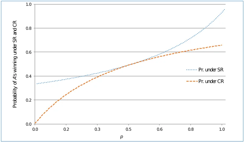
Figure 1: Graph of P rSR(A) and P rCR(A) as a function ofp.
Unlike ELSR, ELCR increases with p, but it approaches infinity at p = 1, because the
tiebreaker never ends when both players alternate successful serves.
3.3
Comparison of Tiebreakers
We compare P rSR(A) and P rCR(A) in Figure 1. Observe that both are increasing in p,
though at different rates. The two curves touch at p= 1
2, where both probabilities equal 1
2. But as p approaches 1, P rSR(A) increases at an increasing rate toward 1, whereas
P rCR(A) increases at a decreasing rate toward 23. Whenp > 1
2,Ahas a greater advantage
under SR, because he is fairly likely to win at the outset with two successful serves, compared to underCR where, if his first serve is successful,B (who has equal probability of success) serves next.
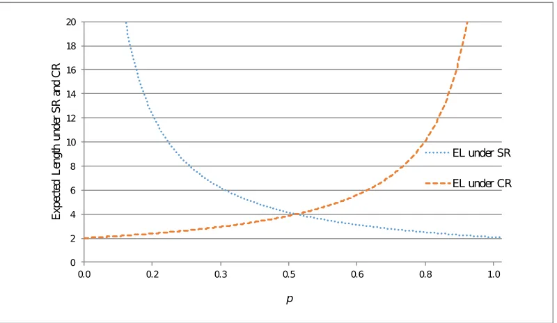
The graph in Figure 2 shows the inverse relationship between ELSR and ELCR as a
function of p. If p = 2
3, which is a realistic value in several service sports, the expected
length of the tiebreaker is greater underCR than underSR (6 vs. 3), which is consistent with our earlier finding for Win-by-One: ELCR > ELSR for Best-of-(2k+ 1) (Theorem 2).
Compared with SR, CR adds 3 serves, on average, to the tiebreaker, and also increases the expected length of the game prior to any tiebreaker, making a tiebreaker that much more likely.
But we emphasize that in the Win-by-One Best-of-(2k+1) game,P rSR(A) =P rCR(A)
(Theorem 1). Thus, compared with SR,CR does not change the probability thatA orB
wins in the regular game. But if there is a tie in this game, the players’ win probabilities may be different in anSRtiebreaker versus a CR tiebreaker. For example, ifp= 2
0 2 4 6 8 10 12 14 16 18 20
0.0 0.2 0.3 0.5 0.6 0.8 1.0
E
x
p
ec
te
d
L
en
g
th
u
n
d
er
S
R
a
n
d
C
R
p
EL under SR
[image:17.612.108.508.78.310.2]EL under CR
Figure 2: Graph of ELSR and ELCR as a function of p.
is the first player to serve in the tiebreaker, he has a probability of 3
5 = 0.600 of winning
under SR and a probability of 4
7 = 0.571 of winning under CR.
3.4
Numerical Comparisons
Clearly, serving first in the tiebreaker is a benefit under both rules. For Best-of-3, we showed in Section 2 that ifp= 2
3, the probability of a tie is 1
3, andB is twice as likely as
A to serve first in the tiebreaker under SR.
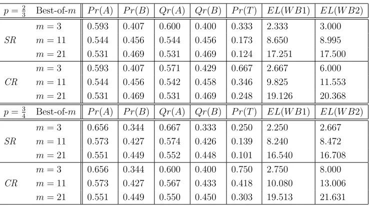
In Table 3, we extend Best-of-3 to the more realistic cases of Best-of-11 and Best-of-21 for both Win-by-One (WB1) and Win-by-Two (WB2) for the cases p = 2
3 and p = 3 4.
Under WB1, the first player to score m = 6 or 11 points wins; under WB2, if there is a 5-5 or 10-10 tie, there is a tiebreaker, which continues until one player is ahead by 2 points.
We compareP rSR(A) andP rCR(A), which assume WB1, with the probabilitiesQrCR(A)
and QrCR(A), which assume WB2, for p = 23 and 3
4. The latter probabilities take into
account the probability of a tie, P r(T), which adjusts the probabilities of A and B’s winning.
For the values of m = 3, 11, and 21 and p = 2 3 and
3
4, we summarize below how the
probabilities of winning and the expected lengths of a game are affected by SR and CR
and Win-by-One and Win-by-Two:
1. Asm increases from m = 3 to 11 to 21, the probability of a tie, P r(T), decreases by more than a factor of two for both p= 2
3 and p= 3
p=2
3 Best-of-m P r(A) P r(B) Qr(A) Qr(B) P r(T) EL(W B1) EL(W B2)
m= 3 0.593 0.407 0.600 0.400 0.333 2.333 3.000
SR m= 11 0.544 0.456 0.544 0.456 0.173 8.650 8.995
m= 21 0.531 0.469 0.531 0.469 0.124 17.251 17.500
m= 3 0.593 0.407 0.571 0.429 0.667 2.667 6.000
CR m= 11 0.544 0.456 0.542 0.458 0.346 9.825 11.553
m= 21 0.531 0.469 0.531 0.469 0.248 19.126 20.368
p=3
4 Best-of-m P r(A) P r(B) Qr(A) Qr(B) P r(T) EL(W B1) EL(W B2)
m= 3 0.656 0.344 0.667 0.333 0.250 2.250 2.667
SR m= 11 0.573 0.427 0.574 0.426 0.139 8.240 8.472
m= 21 0.551 0.449 0.552 0.448 0.101 16.540 16.708
m= 3 0.656 0.344 0.600 0.400 0.750 2.750 8.000
CR m= 11 0.573 0.427 0.567 0.433 0.418 10.080 13.006
[image:18.612.122.491.76.282.2]m= 21 0.551 0.449 0.550 0.450 0.303 19.513 21.631
Table 3: Probability (P r) thatA Wins and B Wins in Best-of-m, and (Qr) thatAWins and B Wins in Best-of-m with a tiebreaker, and that the tiebreaker is implemented (T), and Expected Length of a game (EL), for p= 2
3 and 3 4.
P r(T) is always at least 12% for SR and at least 25% for CR, indicating that, especially for CR, Win-by-Two will often end in a tiebreaker.
2. For p = 2
3, the probability of a tie, P r(T), is twice as great under CR as SR; it
is three times greater for p = 3
4. Thus, games are much closer under CR than SR
because of the much greater frequency of ties under CR.
3. For Best-of-11 and Best-of-21, the probability of A’s winning under Win-by-One (P r(A)) and Win-by-Two (Qr(A)) falls within a narrow range (53–57%), whether
CR or SR is used, echoing Theorem 1 that P r(A) for CR and SR are equal for Win-by-One. They stay quite close for Win-by-Two.
4. The expected length of a game, EL, is always greater under Win-by-Two than under Win-by-One. Whereas EL for Win-by-Two never exceeds EL for Win-by-One by more than one game under SR, under CR this difference may be two or more games, whether p = 2
3 or 3
4. Clearly, the tiebreaker under Win-by-Two may
significantly extend the average length of a game under CR, rendering the game more competitive.
All the variable-rule service sports mentioned in Section 1—except for racquetball, which uses Win-by-One—currently use SR coupled with Win-by-Two. The normal win-ning score of a game in squash is 11 (Best-of-21) and of badminton is 21 (Best-of-41), but a tiebreaker comes into play when there is a tie at 10-10 (squash) or 20-20 (badminton).10
10
In volleyball, the winning score is usually 25; in a tiebreaker it is the receiving team, not the serving team, that is advantaged, because it can set up spike as a return, which is usually successful [13].
The winning score in racquetball is 15, but unlike the other variable-rule service sports, a player scores points only when he or she serves, which prolongs games if the server is unsuccessful. This scoring rule was formerly used in badminton, squash, and volleyball, lengthening games in each sport by as much as a factor of two. The rule was abandoned because this prolongation led to problems in tournaments and discouraged television coverage [3, p. 103]. We are not sure why it persists in racquetball, and why this is apparently the only service sport to use Win-by-One.
We believe that all the aforementioned variable-rule service sports would benefit from
CR. Games would be extended and, hence, be more competitive, without significantly altering win probabilities. Specifically, CR gives identical win probabilities to SR under Win-by-One, and very similar win probabilities under Win-by-Two.
4
The Fixed Rules of Table Tennis and Tennis
Both table tennis and tennis use Win-by-Two, but neither uses SR. Instead, each uses a fixed rule. In table tennis, the players alternate, each serving on two consecutive points, independent of the score and of who wins any point. The winning score is 11 unless there is a 10-10 tie, in which case there is a Win-by-Two tiebreaker, in which the players alternate, but serve on one point instead of two.
There would be little or no advantage to serving first (on two points) in table tennis if there were little or no advantage to serving, as seems to be the case. Ifp= 1
2, the playing
field is level, so neither player gains a probabilistic advantage from being the first double server.
Tennis is a different story.11
It is generally acknowledged that servers have an advan-tage, perhaps ranging from aboutp= 3
5 top= 3
4 in a professional match. In tennis, points
are organized into games, games into sets, and sets into matches. Win-by-Two applies to games and sets. In the tiebreaker for sets, which occurs after a 6-6 tie in games, one player begins by serving once, after which the players alternate serving twice in a row.12
A tennis tiebreaker begins with one player—for us, A—serving. Either A wins the point or B does. Regardless of who wins the first point, there is now a fixed alternating sequence of double serves, BBAABB . . ., for as long as is necessary (see the rule for winning in the next paragraph). When A starts, the entire sequence can be viewed as one of two alternating single serves, broken by the slashes shown below,
AB/BA/AB/BA . . . .
11
Part of this section is adapted from [5].
12
Between each pair of adjacent slashes, the order of A and B switches as one moves from left to right. We call the serves between adjacent slashes a block.
The first player to score 7 points, and win by a margin of at least two points, wins the tiebreaker. Thus, if the players tie at 6-6, a score of 7-6 is not winning. In this case, the tiebreaker would continue until one player goes ahead by two points (e.g., at 8-6, 9-7, etc.).
Notice that, after reaching a 6-6 tie, a win by one player can occur only after the players have played an even number of points, which is at the end of anAB orBA block. This ensures that a player can win only by winning twice in a block—once on the player’s own serve, and once on the opponent’s. The tiebreaker continues as long as the players continue to split blocks after a 6-6 tie, because a player can lead by two points only by winning both serves in a block. When one player is finally ahead by two points, thereby winning the tiebreaker, the players must have had exactly the same number of serves.
The fixed order of serving in the tennis tiebreaker, which is what precludes a player from winning simply because he or she had more serves, is not the only fixed rule that satisfies this property. The strict alternation of single serves,
AB/AB/AB/AB . . . ,
or what Brams and Taylor [4] call “balanced alternation,”
AB/BA/BA/AB . . . ,
are two of many alternating sequences that create adjacent AB or BA blocks.13
All are fair—they ensure that the losing player does not lose only because he or she had fewer serves—for the same reason that the tennis sequence is fair.14
Variable-rule service sports, including badminton, squash, racquetball, and volleyball, do not necessarily equalize the number of times the two players or teams serve. Under
SR, ifA holds his serve throughout a game or a tiebreaker, he can win by serving all the time.
This cannot happen underCR, becauseAloses his serve when he wins; he can hold his serve only when he loses. But this is not to say that Acannot win by serving more often. For example, in Best-of-3 CR,A can beatB 2-1 by serving twice. But the tiebreaker rule in tennis, or any other fixed rule in which there are alternating blocks of AB and BA, does ensure that the winner did not benefit by having more serves.
13
Brams and Taylor [4, p. 38] refer to balanced alternation as “taking turns taking turns taking turns . . .” This sequence was proposed and analyzed by several scholars, and is also known as the Prouhet– Thue–Morse (PTM) sequence [10, pp. 82–85]. Notice that the tennis sequence maximizes the number of double repetitions when written asA/BB/AA/BB/ . . ., because after the first serve by one player, there are alternating double serves by each player. This minimizes changeover time and thus the “jerkiness” of switching servers.
14
5
Summary and Conclusions
We have analyzed four rules for service sports—including the Standard Rule (SR) cur-rently used in many service sports—that make serving variable, or dependent on a player’s (or team’s) previous performance. The three new rules we analyzed all give a player, who loses a point or falls behind in a game, the opportunity to catch up by serving, which is advantageous in most service sports. The Catch-Up Rule (CR) gives a player this oppor-tunity if he or she just lost a point—instead of just winning a point, as under SR. Each of the Trailing Rules (TRs) makes the server the player who trails; if there is a tie, the server is the player who previously was ahead (TRa) or behind (TRb).
For Win-by-One, we showed that SR and CR give the players the same probability of a win, independent of the number of points needed to win. We proved, and illustrated with numerical calculations, that the expected length of a game is greater underCR than under SR, rendering it more likely to stay close to the end.
By contrast, the two TRs give the player who was not the first server, B, a greater probability of winning, making it less likely that they would be acceptable to strong players, especially those who are used to SR and have done well under it. In addition,
TRb is not strategy-proof: We exhibited an instance in which a player can benefit by deliberately losing, which also makes it less appealing.
We analyzed the effects of Win-by-Two, which most service sports currently combine with SR, showing that it is compatible with CR. We showed that the expected length of a game, especially under CR, is always greater under Win-by-Two than Win-by-One.
On the other hand, Win-by-Two, compared with Win-by-One, has little effect on the probability of winning (compareQr(A) and Qr(B) with P r(A) and P r(B) in Table 3).15
The latter property should make CR more acceptable to the powers-that-be in the differ-ent sports who, generally speaking, eschew radical changes that may have unpredictable consequences. But they want to foster competitiveness in their sports, which CR does.
Table tennis and tennis use fixed rules for serving, which specify when the players serve and how many serves they have. We focused on the tiebreaker in tennis, showing that it was fair in the sense of precluding a player from winning simply as a result of having served more than his or her opponent. CR does not offer this guarantee in variable-rule sports, although it does tend to equalize the number of times that each player serves.
There is little doubt that suspense is created, which renders play more exciting and unpredictable, by making who serves next dependent on the success or failure of the server—rather than fixing in advance who serves and when. But a sport can still generate keen competition, as the tennis tiebreaker does, even with a fixed service schedule. Thus, the rules of tennis, and in particular the tiebreaker, seem well-chosen; they create both fairness and suspense.
15
6
Appendix
6.1
Theorem 1:
SR
and
CR
Give Equal Win Probabilities
We define a serving schedule for a Best-of-(2k+ 1) game to be
(A1, . . . , Ak+1, B1, . . . , Bk)∈ {W, L}
2k+1
,
where for i = 1,2, . . . , k+ 1, Ai records the result of A’s ith serve, with W representing
a win for A and La loss forA, and for j = 1,2, . . . , k, Bj represents the result ofB’sjth
serve, where now W represents a win for B and Lrepresents a loss for B.
The order in which random variables are determined does not influence the result of a game. So we may as well let A and B determine their service schedule in advance, and then play out their game under SR or CR, using the predetermined result of each serve.
The auxiliary rule, AR, is a serving rule for a Best-of-(2k+ 1) game in whichA serves
k+ 1 times consecutively, and then B serves k times consecutively. For convenience, we can assume that AR continues for 2k+ 1 serves, even after one player accumulatesk+ 1 points. The basis of our proof is a demonstration that, if the serving schedule is fixed, then games played under all three serving rules, AR, SR, and CR, are won by the same player.
Theorem 1. Let k ≥1. In a Best-of-(2k+ 1) game, P rSR(A) =P rCR(A).
Proof. Suppose we have already demonstrated that, for any serving schedule, the three service rules—AR, SR, and CR—all give the same winner. It follows that the subset of service schedules under whichA wins underSRmust be identical to the subset of service schedules under which A wins under CR. Moreover, regardless of the serving rule, any serving schedule that contains n wins for A as server and m wins for B as server must be associated with the probability pn(1−p)k+1−nqm(1−q)k−m.16
Because the probability that a player wins under a service rule must equal the sum of the probabilities of all the service schedules in which the player wins under that rule, the proof of the theorem will be complete.
Fix a serving schedule (A1, . . . , Ak+1, B1, . . . , Bk)∈ {W, L}2k+1. Leta be the number
of A’s server losses andb be the number ofB’s server losses. (For example, fork = 2 and serving schedule (W, L, L),a= 1 and b= 1.)
Under service rule AR, there are 2k + 1 serves in total. Then A must accumulate
k+ 1 +b−a points andB must accumulate k−b+a points. Clearly,A has strictly more points than B if and only if b≥a.
Now consider service ruleSR, under which service switches whenever the server loses. First we prove that, if b ≥ a, A will have the opportunity to serve at least k + 1 times.
16
What really matters is that any serving schedule is associated with some probability. For example, as discussed in footnote 4, ifA wins his ith serve with probabilitypi, fori = 1,2, . . ., and thatB wins
herjth serve with probabilityqj, for j= 1,2, . . ., then the formula would be more complicated, but the
A serves until he loses, and then B serves until she loses, so immediately after B’s first loss, A has also lost once and is to serve next. Repeating, immediately afterB’sath loss,
A has also losta times and is to serve next. Either A’s prior loss was his (k+ 1)st serve, or A wins every serve from this point on, including A’s (k+ 1)st serve. After this serve,
A has k+ 1−a+b ≥k+ 1 points, so A must have won either on this serve or earlier. Now suppose thata > bunder service ruleSR. Then, afterB’sbth loss,Ahas also lost
b times and is to serve. Moreover, A must lose again (since b < a), and then B becomes server and continues to serve (without losing) until B has served k times. By then, B
will have gained k−b+a ≥k+ 1 points, so B will have won. In conclusion, under SR,
A wins if and only if b≥a.
Consider now service rule CR, under whichA serves until he wins, thenB serves until she wins, etc. Clearly, B cannot win a point on her own serve until after A has won a point on his own serve. Repeating, ifB has just won a point on serve, then A must have already won the same number of points on serve asB.
Again assume that b ≥ a. Note that A has k+ 1−a server wins in his first k + 1 serves, B has k−b server wins in her first k serves, and k+ 1−a > k−b. Consider the situation under CR immediately after B’s (k −b)th server win. (All of B’s serves after this point up to and including the kth serve must be losses.) At this point, both A and
B have k−b server wins. Suppose that A also has a′ ≤ a server losses, and that B has b′ ≤b server losses. Then the score at this point must be (k−b+b′, k−b+a′).
Immediately afterB’s (k−b)th server win,Ais on serve. ForA, the schedule up toA’s (k+1)st serve must containa−a′ server losses andk+1−a−(k−b) =b−a+1>0 server
wins. Immediately after A’s next server win, which is A’s (k−b+ 1)st server win, A’s score isk−b+b′+ 1, andB’s score is at most k−b+a′+ (a−a′) =k−b+a ≤k. Then B
is on serve, and all ofB’sb−b′ remaining serves (up to and includingB’skth serve) must
be server losses. Therefore, afterB’skth serve,A’s score isk−b+b′+ 1 + (b−b′) =k+ 1,
and A wins.
If b < a, an analogous argument shows that B wins under CR. This completes the
proof that, under any serving schedule, the winner under AR is the same as the winner under SR and under CR.
6.2
Theorem 2: Expected Lengths under
SR
and
CR
Lemma 1. Let 1≤t≤s≤r. If a subset ofs dots is selected uniformly from a sequence of r dots, the expected position of the tth selected dot in the full sequence is
t
r+ 1
s+ 1
.
Proof. If i is any nonselected dot, let Xi be an indicator variable such that Xi = 1 if
dot i precedes the tth selected dot, and Xi = 0 otherwise. Then E[Xi] = P(Xi = 1)
and the expected position of thetth dot is E[P
iXi] +t, where the sum is taken over all
nonselected dots.
Now P(Xi = 1) depends only on the position of dot i and the s selected dots;
tth position. In other words, for any nonselected dot i, P(Xi = 1) = s+1t . Therefore, the
expected position of the tth dot is (r−s) t
s+1 +t=t
r+1
s+1, as required.
Theorem 2. If 0 < p < 1, 0 < q < 1, and k ≥ 1, then the expected length of
Best-of-(2k+ 1) game under CR is greater than under SR if and only if p+q >1.
Proof. As defined earlier, a service schedule is a sequence of exactlyk+1 wins and losses on
A’s serves and exactlyk wins and losses onB’s serves. A service schedule has parameters (n, m) if it containsn server wins forA and m server wins forB. The probability of any particular service schedule with parameters (n, m) is
P r0(n, m) =pn(1−p)k +1−n
qm(1−q)k−m.
The probability that some service schedule with parameters (n, m) occurs is
P r(n, m) =
k+ 1
n
k m
pn(1−p)k+1−nqm(1−q)k−m.
Consider a service schedule with parameters (n, m). Using SR, if n > m, thenA wins and exhausts his part of the service schedule. B uses her part of the schedule through her (k+ 1−n)th loss. From Lemma 1 withr=k,s=k−m,t =k+ 1−n, the expected length of the game is
EL0
SR(n, m) = k+ 1 + (k+ 1−n)
k+ 1
k+ 1−m
= 2(k+ 1)−(n−m)
m
k+ 1−m + 1
.
However, if n ≤ m, then B wins and exhausts her part of the service schedule, while A
uses his part of the schedule through his (k+1−m)th loss. From Lemma 1 withr=k+1,
s=k+ 1−n, t =k+ 1−m, the expected length of the game is
EL0
SR(n, m) = k+ (k+ 1−m)
k+ 1 + 1
k+ 1−n+ 1
= 2(k+ 1)−(m−n+ 1)
n
k+ 1−n+ 1 + 1
.
Using CR, if n > m, then A wins, B exhausts her part of the service schedule, and
A uses his schedule through his (m+ 1)st win. From Lemma 1 with r = k+ 1, s = n,
t=m+ 1, the expected length of the game is
EL0
CR(n, m) = k+ (m+ 1)
k+ 1 + 1
n+ 1
= 2(k+ 1)−(n−m)
k+ 1−n
n+ 1 + 1
But if n ≤ m, then B wins, A exhausts his part of the service schedule, and B uses her part through her nth win. From Lemma 1 withr =k, s=m,t =n, the expected length of the game is
EL0
CR(n, m) =k+ 1 +n
k+ 1
m+ 1
= 2(k+ 1)−(m−n+ 1)
k−m
m+ 1 + 1
.
Combining the first two formulas, we can write the expected length of a game played under SR, 17
ELSR =
X
n>m
P r(n, m)
2(k+ 1)−(n−m)
m
k+ 1−m + 1
+X
n≤m
P r(n, m)
2(k+ 1)−(m−n+ 1)
n
k+ 1−n+ 1 + 1
,
and the expected length of a game played under CR,
ELCR =
X
n>m
P r(n, m)
2(k+ 1)−(n−m)
k+ 1−n
n+ 1 + 1
+X
n≤m
P r(n, m)
2(k+ 1)−(m−n+ 1)
k−m
m+ 1 + 1
.
When we subtract these expressions, many terms cancel:
ELCR−ELSR =
X
n>m
P r(n, m)(n−m)
m
k+ 1−m −
k+ 1−n
n+ 1
+X
n≤m
P r(n, m)(m−n+ 1)
n
k+ 1−n+ 1 −
k−m
m+ 1
.
Our objective now is to show that this quantity, the expected number of points by which the length of aCR game exceeds the length of anSRgame, has the same sign asp+q−1. To simplify this expected difference in lengths, we extract the binomial coefficients
k+1
n
and mk
from the probability factors and use the following identities:
k m
· m
k+ 1−m =
k
m−1
;
k+ 1
n
· k+ 1−n
n+ 1 =
k+ 1
n+ 1
;
k+ 1
n
· n
k+ 1−n+ 1 =
k+ 1
n−1
; k m
· k−m
m+ 1 =
k
m+ 1
.
17
We take the sumP
n>m to include terms for every integer pair (n, m) withn > m. Ifn > k+ 1 or
m > k, we takeP r(n, m) = 0, so the sum includes only finitely many nonzero terms. Similarly, the sum P
n≤m includes terms for every integer pair (n, m) withn ≤m. In general, we interpret the binomial
coefficient a
The result is
ELCR−ELSR
= X
n>m
P r0(n, m)(n−m)
k+ 1
n
k
m−1
−
k+ 1
n+ 1
k m +X n≤m
P r0(n, m)(m−n+ 1)
k+ 1
n−1
k m −
k+ 1
n
k
m+ 1
.
Now split the sums to obtain
ELCR−ELSR =
X
n>m
P r0(n, m)(n−m)
k+ 1
n
k
m−1
− X
n>m
P r0(n, m)(n−m)
k+ 1
n+ 1
k m +X n≤m
P r0(n, m)(m−n+ 1)
k+ 1
n−1
k m −X n≤m
P r0(n, m)(m−n+ 1)
k+ 1
n
k
m+ 1
.
To analyze the expression for ELCR − ELSR, we first shift indices in the second
summation by replacing nbyn−1 andm bym−1 throughout. Of course, the condition
n > m and the factor n−m are not affected. Then
X
n>m
P r0(n, m)(n−m)
k+ 1
n+ 1
k m = X n>m
P r0(n−1, m−1)(n−m)
k+ 1
n
k
m−1
= 1−p
p
1−q q
X
n>m
P r0(n, m)(n−m)
k+ 1
n
k
m−1
,
where in the last step we have used the relationship
P r0(n−1, m−1) =
1−p p
1−q
q P r0(n, m)
in the end the fourth summation matches the third.
X
n≤m
P r0(n, m)(m−n+ 1)
k+ 1
n
k
m+ 1
= X
n≤m
P r0(n−1, m−1)(m−n+ 1)
k+ 1
n−1
k m
= 1−p
p
1−q q
X
n≤m
P r0(n, m)(m−n+ 1)
k+ 1
n−1
k m
.
Incorporating these changes into our expression for ELCR−ELSR gives
ELCR−ELSR
=
1− 1−p
p
1−q q
X
n>m
P r0(n, m)(n−m)
k+ 1
n
k
m−1
+
1− 1−p
p
1−q q
X
n≤m
P r0(n, m)(m−n+ 1)
k+ 1
n−1
k m
.
This completes the proof, because the sums include only positive terms, and the common factor is
1− 1−p
p
1−q
q =
p+q−1
pq ,
which has the same sign as p+q−1.
6.3
Theorem 3: Strategy-proofness of
TRa
Theorem 3. TRb is strategy-vulnerable, whereas SR and CR are strategy-proof. TRa is strategy-proof whenever p+q >1.
See Section 2 for the proof that TRb is strategy-vulnerable and that SR and CR are strategy-proof. Here we consider only a Best-of-(2k+ 1) game played under TRa, and use notation similar to the text: (C, x, y) denotes a state in which player C (C =A orB) is about to serve,A’s current score isx, andB’s isy. LetWA(C, x, y) denoteA’s conditional
win probability given that the game reaches state (C, x, y). Assume thatp+q >1. Given any state, call the state that was its immediate predecessor itsparent. Call two states siblings if they have the same parent. For example, state (A,0,0) is the parent of siblings (B,1,0) and (A,0,1). Let 0< x≤k+ 1 and 0≤y≤k+ 1 withx+y≤2k+ 1. Then any state (C, x, y) must have a sibling (C′, x−1, y+ 1), namely the state that would
have arisen had B, and not A, won the last point.
To show that the Best-of-(2k+ 1) game played under TRa is strategy-proof forA, we must show thatWA(C, x, y)≥WA(C′, x−1, y+ 1) whenever (C, x, y) and (C′, x−1, y+ 1)
if y =k+ 1, where C =A or B. In these cases, (C, x, y) is a terminal state and can be written (x, y), as there are no more serves.
Lemma 2. Suppose that x6=y and the state is (C, x, y). Then either x < y and C =A, or x > y and C =B.
Proof. UnderTRa, the player about to serve must be the player with the lower score.
Lemma 3. The states (A, x, y) and (B, x, y) can both arise if and only if 0 < x = y < k+ 1. In this case, the state is (A, x, x) if the parent was (B, x, x−1), and the state is
(B, x, x) if the parent was (A, x−1, x).
Proof. The first statement follows from Lemma 2. The second is a paraphrase ofTRa.
Note that Lemma 3 fails for TRb; in fact, it captures the difference betweenTRa and
TRb. For example, under TRb, if A loses at (B,1,0), the next state will be (B,1,1) (it would be (A,1,1) under TRa), and if A wins at (A,0,1), the next state will be (A,1,1) (rather than (B,1,1) under TRa).
Lemma 4. WA(A, x, x)> WA(B, x, x) if and only if
WA(B, x+ 1, x)> WA(A, x, x+ 1).
Proof. First notice that WA(A, x, x) = pWA(B, x+ 1, x) + (1− p)WA(A, x, x+ 1) and WA(B, x, x) = (1−q)WA(B, x+ 1, x) +qWA(A, x, x+ 1). Therefore
WA(A, x, x)−WA(B, x, x) = (p+q−1) [WA(B, x+ 1, x)−WA(A, x, x+ 1)]
and the claim follows from the assumption that p+q >1.
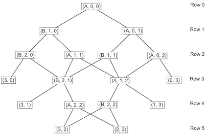
We now consider the probability tree of a Best-of-(2k+ 1) game played under TRa. The Best-of-5 tree (k= 2) is shown in Figure 3. The nodes (states) are labeled (C, x, y), whereC is the player to serve, xis the score of A, andy is the score ofB. Because there are no servers after the game has been won, the terminal nodes are labeled either (k+1, y) or (x, k+ 1). The probability tree is rooted at (A,0,0) and is binary—every nonterminal node is parent to exactly two nodes. For nonterminal nodes whereA serves, the left-hand outgoing arc has probability p and the right-hand outgoing arc has probability 1−p; for nonterminal nodes where B serves, the two outgoing arcs have probability 1−q and q, respectively.
The probability tree for the Best-of-(2k+ 1) game played underTRa has 2k+ 2 rows, numbered 0 (at the top) to 2k+ 1 (at the bottom). The top row contains only the initial state, (A,0,0), and the bottom row contains only terminal nodes. At every node in row
ℓ, the players’ scores sum to ℓ.
(A, 0, 0)
(A, 0, 1)
(A, 0, 2)
(B, 2, 2) (A, 1, 2) (B, 1, 0)
(A, 1, 1) (B, 1, 1)
(B, 2, 0)
(3, 0)
(3, 1)
(3, 2) (2, 3)
(1, 3) (0, 3)
(A, 2, 2) (B, 2, 1)
Row 0
Row 1
[image:29.612.105.508.74.338.2]Row 5 Row 4 Row 3 Row 2
Figure 3: Best-of-5 TRa probability tree.
show that row ℓ contains ℓ+ 2 states, from (B, ℓ,0) to (A,0, ℓ), including both (A, ℓ
2,
ℓ
2)
and (B, ℓ
2,
ℓ
2). We place (A,
ℓ
2,
ℓ
2) to the left of (B,
ℓ
2,
ℓ
2).
In the lower half of the tree—row k+ 1 and below—each row begins and ends with a terminal node. Letk+ 1≤ℓ≤2k+ 1. Then the first entry in rowℓis the terminal node (k+ 1, ℓ−k−1), and the last entry is the terminal node (ℓ−k−1, k+ 1). Ifℓis odd, every nonterminal node in row ℓ is a state of the form (C, x, ℓ−x) for x =k, k−1, . . . , ℓ−k. (If ℓ = 2k + 1, the only nodes in row ℓ are two terminal nodes.) By Lemma 2, row ℓ
contains 2k−ℓ+ 3 nodes in total. Ifℓ is even, row ℓ contains 2k−ℓ+ 4 nodes, from the terminal node (k, ℓ−k) to the terminal node (ℓ −k, k), including all possible states of the form (C, x, ℓ−x) for x = k, k−1, . . . , ℓ−k. Among these states are both (A, ℓ
2,
ℓ
2)
and (B, ℓ
2,
ℓ
2), with the former state on the left.
As the figure illustrates, sibling states have a unique parent unless they are of the form (B, x+ 1, x) and (A, x, x+ 1), in which case both (A, x, x) and (B, x, x) are parents. Thus, (B, x+ 1, x) and (A, x, x+ 1) could be called “double siblings.”
The method of proof is to show by induction that the function WA(·) is decreasing on
each row as one reads from left to right. This will prove thatTRa is strategy-proof forA, because it will show that, in every state,A does better by winning the next point rather than losing it to obtain the sibling state. Since WB(·) = 1−WA(·), the proof also shows
that WB(·) is increasing on each row, and therefore that TRa is strategy-proof for B.
node (k+1, k−1), whereWA(k+1, k−1) = 1, and ends with a terminal node (k−1, k+1),
whereWA(k−1, k+ 1) = 0. Row 2k contains 4 nodes; its second entry is (A, k, k) and its
third is (B, k, k). To apply Lemma 4 with x=k, note that (B, k+ 1, k) and (A, k, k+ 1) are the terminal nodes (k+ 1, k) and (k, k+ 1), and WA(k+ 1, k) = 1 > WA(k, k+ 1) = 0.
Lemma 4 now implies that WA(A, k, k)> WA(B, k, k), as required.
Now consider any row ℓ, and assume that WA(·) has been shown to be strictly
de-creasing on row ℓ+ 1. Ifℓ ≥k+ 1, rowℓ begins and ends with a terminal node, for which
WA(k+ 1, ℓ−k−1) = 1 and WA(ℓ−k−1, k+ 1) = 0; any other node in row ℓ is a
nonterminal node. Suppose that (C, x, ℓ−x) and (C′, x′, ℓ−x′) are adjacent nodes in row ℓand that (C, x, ℓ−x) is on the left. First suppose thatx=x′. Then by Lemma 3,ℓmust
be even, and the two nodes must be (A, ℓ
2,
ℓ
2) (on the left) and (B,
ℓ
2,
ℓ
2) (on the right).
The induction assumption and Lemma 4 now implies that WA(A,2ℓ,
ℓ
2)> WA(B,
ℓ
2,
ℓ
2).
Otherwise, consecutive nodes (C, x, ℓ−x) and (C′, x′, ℓ−x′) in row ℓ must satisfy x′ =x−1, by Lemmata 2 and 3. Thus we are comparingW
A(C, x, ℓ−x) withWA(C′, x−
1, ℓ−x+ 1). Now
WA(C, x, ℓ−x) =rWA(D, x+ 1, ℓ−x) + (1−r)WA(D′, x, ℓ−x+ 1) > WA(D′, x, ℓ−x+ 1),
WA(C′, x−1, ℓ−x+ 1)
=sWA(E, x, ℓ−x+ 1) + (1−s)WA(E′, x−1, ℓ−x+ 2) > WA(E, x, ℓ−x+ 1),
where 0 < r, s <1 because each of r and s must equal one of p, q, 1−p, and 1−q. According to Lemma 3, (D′, x, ℓ−x+ 1) = (E, x, ℓ−x+ 1) unless x=ℓ−x+ 1, i.e., x = ℓ+1
2 (which of course requires that ℓ be odd). First assume that x 6=
ℓ+1
2 . Then we
have shown that
WA(C, x, ℓ−x)> WA(D′, x, ℓ−x+ 1)
=WA(E, x, ℓ−x+ 1)> WA(C′, x−1, ℓ−x+ 1),
as required.
Now assume thatx= ℓ+1
2 . Then the original states (C, x, ℓ−x) and (C
′, x−1, ℓ−x+1)
must have been (B,ℓ+1 2 ,
ℓ−1
2 ) and (A,
ℓ−1
2 ,
ℓ+1
2 ). Moreover, (D
′, x, ℓ−x+ 1) = (A,ℓ+1 2 ,
ℓ+1
2 )
and (E, x, ℓ −x+ 1) = (B,ℓ+1 2 ,
ℓ+1
2 ). Recall that (A, x, x) always appears to the left
of (B, x, x). Thus the assumption that WA(·) is decreasing on row ℓ + 1 implies that WA(A,ℓ+12 ,
ℓ+1
2 )> WA(B,
ℓ+1
2 ,
ℓ+1
2 ). By Lemma 4, we have shown that
WA(B, ℓ+ 1
2 ,
ℓ−1
2 )> WA(A,
ℓ+ 1 2 ,
ℓ+ 1 2 )
> WA(B, ℓ+ 1
2 ,
ℓ+ 1
2 )> WA(A,
ℓ−1 2 ,
ℓ+ 1 2 ), completing the proof of Theorem 3.