Original Article Classification of MRI and psychological testing data based on support vector machine

Original Article

Classification of MRI and psychological testing data

based on support vector machine

Wenlu Yang1_{, Xinyun Chen}1_{, David S Cohen}2_{, Eric R Rosin}2_{, Arthur W Toga}3_{, Paul M Thompson}3_{, Xudong} Huang2_{, For the Alzheimer’s Disease Neuroimaging Initiative}*

1_{Department of Electrical Engineering, Information Engineering College, Shanghai Maritime University, Shanghai,}

China; 2_{Neurochemistry Laboratory, Department of Psychiatry, Massachusetts General Hospital and Harvard}

Medical School, Charlestown, MA, USA; 3_{Laboratory of Neuro Imaging, The Mark and Mary Stevens}

Neuroimag-ing and Informatics Institute, Keck School of Medicine of USC, University of Southern California, Los Angeles, CA, USA; *_{Data used in preparation of this article were obtained from the Alzheimer’s Disease Neuroimaging}

Initiative (ADNI) database (adni.loni.usc.edu). As such, the investigators within the ADNI contributed to the design and implementation of ADNI and/or provided data but did not participate in analysis or writing of this report. A complete listing of ADNI investigators can be found at: http://adni.loni.usc.edu/wpcontent/uploads/how_to_ap-ply/ADNI_Acknowledgement_List.pdf.

Received November 6, 2017; Accepted November 21, 2017; Epub December 15, 2017; Published December 30, 2017

Abstract: Alzheimer’s disease (AD) is a progressive, and often fatal, brain disease that causes neurodegeneration, resulting in memory loss as well as other cognitive and behavioral problems. Here, we propose a novel multimodal method combining independent components from MRI measures and clinical assessments to distinguish Alzheimer’s patients or mild cognitive impairment (MCI) subjects from healthy elderly controls. 70 AD subjects (mean age: 77.15 ± 6.2 years), 98 MCI subjects (mean age: 76.91 ± 5.7 years), and 150 HC subjects (mean age: 75.69 ± 3.8 years) were analyzed. Our method includes the following steps: pre-processing, estimating the number of independent components from the MR image data, extracting effective voxels for classification, and classification using a support vector machine (SVM)-based classifier. As a result, with regards to classifying AD from healthy controls, we achieved a classification accuracy of 97.7%, sensitivity of 99.2%, and specificity of 96.7%; for differentiating MCI from healthy controls, we achieved a classification accuracy of 87.8%, a sensitivity of 86.0%, and a specificity of 89.6; these results are better than those obtained with clinical measurements alone (accuracy of 79.5%, sensitivity of 74.0%, and specificity of 85.1%). We found that (1) both AD patients and MCI subjects showed brain tissue loss, but the volumes of gray matter loss in MCI subjects was far less, supporting the notion that MCI is a prodromal stage of AD; and (2) combining gray matter features from MRI and three commonly used measures of mental status, cognitive function improved classification accuracy, sensitivity, and specificity compared with classification using only independent components or clinical measurements.

Keywords: Alzheimer’s disease, mild cognitive impairment, structural MRI, source-based morphometry, indepen-dent component analysis, support vector machine

Introduction

The most common form of dementia, accoun-

ting for 50% to 80% of dementia cases, is

Alzheimer’s disease (AD). AD is a progressive, and often fatal, brain disease that causes neu-rodegeneration, resulting in memory loss as well as other cognitive and behavioral prob- lems that are often severe enough to affect all aspects of a person’s life. Effective and va- lid early diagnosis is vital for the slowing and, ultimately, the prevention of disease

progres-sion. A variety of biomedical imaging techni- ques such as structural or functional magne- tic resonance imaging (sMRI/fMRI) [1-10] and positron emission tomography (PET) [11-14] are being used to assess AD patients. sMRI is

a noninvasive and efficient technology, and

on specific brain regions, especially the hippo -campus and entorhinal cortex [21-24]. By com-paring regional volumes of ROIs across diag-nostic groups, researchers have uncovered va- luable information about the patterns of mor-phometric differences, and have laid the foun-dation for subsequent studies for which

voxel-based morphometry (VBM) [25, 26] and

ten-sor-based morphometry (TBM) [27] are widely used methods to calculate tissue changes with mathematically complex voxel-wise modeling [28, 29]. ROI-based analyses falls short in

sev-eral respects: first, they typically only consider

a spatially limited region of the subject’s brain, neglecting much of the available information, which may be important [30]. Second, when univariate analyses are used, they are incapa-ble of including the joint information among voxels in a 3D image and are often less effec-tive at analyzing individual subjects. Although largely prevalent in univariate tests, some multi-ROI studies have been done.

By contrast, multivariate methods consider the relationship among voxels; they may also con-sider volumes of several prior regions of

inter-est, segmented manually or automatically.

Vo-xels with a similar attribute may be aggregated into one group, and all of these voxels make up a source. Inspired by the source concept, so- urce-based morphometry (SBM) [31, 32] was

developed from VBM with four key steps:

pre-processing, ICA, statistical analysis, and sta- tistical mapping. Before we actually perform ICA as a requirement of SBM, we need to esti-mate the number of independent components. This involves testing the eigenvalues of a sa- mple covariance matrix in order to estimate the number of the equal smallest eigenvalues of the true covariance matrix that is based on the information theoretic criterion (ITC) [33]. Classifying patients as AD versus normal is also a major goal in the diagnosis of AD. We begin by describing how to extract features from different groups of subjects. In diverse

applications across various fields, support ve-ctor machines (SVMs) turn out to be one of

the most effective feature extraction methods

[34-38] that can be mathematically simplified

using optimization techniques [39].

In this paper, we first describe the methods

used in our experiments and the cohort studied in the Methods section. Results of our analyses are detailed in the results section, followed by a discussion and conclusion.

Materials and methods

Magnetic resonance images

Data used in the preparation of this article were obtained from the Alzheimer’s Disease NeuroimagingInitiative (ADNI) database (adni. loni.usc.edu). The ADNI was launched in 2003 as a public-private partnership, led by Principal Investigator Michael W. Weiner, MD. The pri- mary goal of ADNI has been to test whether se- rial magnetic resonance imaging (MRI), posi-tron emission tomography (PET), otherbiologi-cal markers, and cliniotherbiologi-cal and neuropsychologi-cal assessment can be combined to measure the progression of mild cognitive impairment (MCI) and early Alzheimer’s disease (AD). The MRI data used in this paper is from the Alzheimer’s Disease Neuroimaging Initiative (ADNI), which has recruited over 800 adults, aged 55 to 90, from 55 initially planned sites across the United States and Canada [40] (la- ter extended to 59 sites) [41]. In the initial stage of the study, approximately 200 cogni-tively normal individuals were followed for th- ree years; 400 subjects with MCI were fol- lowed for three years; and 200 patients with early AD were followed for two years. Later on, these time periods were extended and more subjects were added [42]. Quality control pro-cedures were applied to ensure that the cor- rect scan protocol, orientation, and angula- tions were used [40]. ADNI data has been

classified using SVMs in the past [43].

In our study we chose the 1.5 T T1-weighted MRI screening scans that can be used as ba- seline scans for our following research sub- jects with the MRIs in which extreme detect- ed deformations were excluded. We randomly picked MRIs and constructed three groups of MRIs: group AD included 70 MRI images of AD patients, group MCI was composed of 98 sub-jects with MCI, and 150 cognitively normal indi-viduals’ MRIs were included in group HC. Each group of MRI gray matter images, segmented from the MRI data [35], shared a similar num-ber of voxels that could clearly be distinguish- ed from an MRI viewer like MRIcro [44], which offers a mean image after preprocessing. Tho- se images with a largely deviated number of voxels were abandoned in advance to improve

classification. The final smoothed gray matter

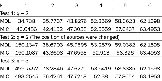
Table 1. Simulation results of MDL and MIC

k 1 2 3 4 5 6

Test 1: q = 2

MDL 34.738 35.7737 43.8276 52.3569 58.3623 62.1698 MIC 43.6486 42.4132 47.3038 52.3559 57.6437 63.4953 Test 2: q = 2 (The position of sources were changed)

MDL 150.1347 38.6703 45.7595 53.2579 59.0382 62.1698 MIC 150.1087 43.3698 47.6558 52.913 58.326 63.4953 Test 3: q = 3

MDL 499.7452 78.2846 47.6271 53.5419 58.8385 62.1698 MIC 483.2545 76.4261 47.7218 52.38 57.8054 63.4953

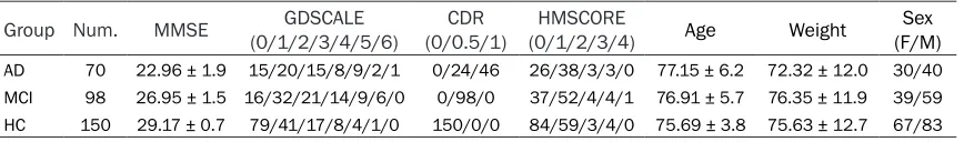
using the SPM8 toolbox that we will discuss later in the preprocessing section. Our goal was to compare AD images with HC ones, and MCI images with HC images, respectively, and draw out features from these comparisons. A brief summary of the participants’ demographics and dementia status is listed in Table 2. This table demonstrates the participants’ statistical gender, age, education, socioeconomic, and clinical dementia rating information. The num-ber of participants in each group is listed in col-umn Num. Corresponding colcol-umns show the mean value of the mini-mental state examina-tion (MMSE), the age and weight of these three groups, and the number of people with the

spe-cific scale value of GDS total score (GDSCALE), CDR, Modified HachinskiIschaemic scale

(HMSCORE), and sex.

Overview

Information theory criteria overview: We intend-ed to use SBM to study MR image data, which involves the procedure of ICA; however, to avoid choosing the number of independent compo-nents randomly and arbitrarily, we calculated the number by a principle method. A commonly used ITC for order selection [45], AIC [46], is developed based on the minimization of the Kullback-Leibler divergence between the true

model and the fitted model. AIC is extended by

Cavanaugh as the Kullback-Leibler information criterion (KIC) [47] using a symmetric

Kullback-Leibler divergence between the true and fitted

models. MDL criterion is developed based on the minimum code length.

Although these two approaches have similar structures, each of them has their own special-ties [48-50]. AIC has the advantage of

perform-ing well for those “difficult” problems when

large eigenvalues are not much bigger than the

smallest eigenvalues, but is inconsistent and tends to overes-timate the model order for the easier cases. MDL on the other hand, performs with extreme reli-ability for most cases but falls short of AIC’s performance for

difficult cases [51]. Here, we

come up with a question: is there any approach that can leverage both criterions’ advantages with-out also absorbing their disad- vantages?

The minimum probability of error criterion (introduced by Douglas B. Williams [48]) based on the theory of multiple hypothesis tests, per-forms better than either AIC or MDL. Here, we

call this approach modified ITC, and symbolize

it as MIC. The equation for MIC can be summa-rized as equation 1:

i

i

MIC( ) ₂1 ( )( ) log( ₁ )

4

k (2T k 1)

k T k n k

T k 1

2 _{1 1}

i i k

T i k 1

T k j T j k T 1 T k

log log ( T ( ))

log log( )

4 ( )

1 1

1/2 p p i

k

j k T

i

k _{i j}

j k j k 2 n 2 2 1 T - - -+ = -+ -m

m v- + + = + = + = = -r m m m m m m m - + = + = -% / / / _{/ /} (1)

In this equation, n is one less than the number of samples and 1

T k 2 1 i i k T = -v -+

=/ m, Tk

^ h is the

multivariate gamma function. To testify the availability of MIC compared to MDL, we make use of the resulting eigenvalues of Mati Wax and Thomas Kailarth’s simulation [33] in which

seven sensors specifically receive data sent by

several sources in different directions and are independently distributed. A hundred samples are extracted from each sensor so that N=100. The number of signal sources (the value of q) is changed to see whether or not MDL and MIC can correctly offer a corresponding estimation of the source number. The results of these tests are displayed in Table 1.

From Test 1, MIC reached a minimal value when k was 2, while MDL was smallest when k was 1. The reason why MDL, in this case, missed the right source number, is that this case is what

of findings pertaining to some particular

ca-ses,a number of morphometric features may

be more difficult to quantify by inspection. While the VBM approach is not biased to one

particular structure, it even-handedly and com-prehensively assesses anatomical differences throughout the brain.

Compared to VBM, which involves the process

of pre-processing, statistical analysis, and

sta-tistical maps, SBM [31] derived from VBM also

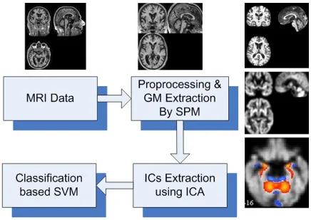
includes ICA between the pre-processing step and the statistical analysis step as shown in Figure 1.

With VBM, the procedure is quite straightfor -ward and generally involves the following two

steps: first, in the pre-processing step it spa -tially normalizes high-resolution images from all the subjects into the same stereotactic space that is followed by segmenting the gray matter from the spatially normalized images and smoothing the gray-matter segments. Second, to do the statistical analysis, voxel-wise parametric statistical tests comparing the smoothed gray matter images from the groups are performed. Corrections for multiple comparisons are made using the theory of

Gaussian random fields.

Identical to VBM, SBM applies the same pro -cess in the pre-pro-cessing step and the stati- stical analysis step with the only difference being that it carries out ICA. ICA is a statistical and computational technique for revealing hid-den factors that underlie sets of random vari-ables, measurements, or signals, before

per-forming statistical analysis. ICA defines a

ge-nerative model for the observed multivariate data that is typically given a large database of samples and, in the model, the data variables are assumed to be linear or a nonlinear mixture of some unknown latent variables; the mixing system is also unknown. The latent variables, called the independent components, sources,

or factors, are assumed non-Gaussian and

mutually independent, and can be found by ICA. As a result, ICA performed here can identi-mentioned above, with which MDL is

ineffec-tive. In Test 2, the position of those two sources was regulated and both criterions received the correct number of 2. In Test 3, one more source was added and after the same calculation. From the results of the three simulations, MIC could correctly identify the right number of sources that we set. MDL failed in Test 1 to expose a shortcoming that needs to be avoid-ed. Although we cannot directly conclude that MIC performs better than AIC in these three simulations, we can say that MIC and MDL share more similarity than MIC and AIC, and that this similarity will guarantee that MIC, like MDL, performs more stably over most cases

that would be certified in the following experi -ment with the subject data. As a result, we decided to use MIC during our study to esti-mate the independent components before we actually carried out ICA.

SBM overview

Deformation-based morphometry (DBM) and TBM are two computational neuro-anatomical methods for studying brain shapes based on

deformation fields obtained by the nonlinear

registration of brain images. When comparing

groups, DBM uses deformation fields to identify

differences in the relative positions of struc-tures within subjects’ brains. TBM can refer to those methods that localize the differences in the local shapes of brain structures and can be used to produce statistical parametric maps of regional shape differences.

VBM is another class of techniques that can

be applied to some scalar function of the

nor-malized image. When VBM is compared with

TBM at small scales that need to compute very

high resolution deformation fields, it is

sim-ple and pragmatic in addressing small-scale

differences [28, 29]. Simply speaking, VBM

involves a voxel-wise comparison of the local concentration of gray matter between two groups of subjects. Although these earlier mor-phometric measurements resulted in a wealth

Table 2. The summary of participants’ clinical status

Group Num. MMSE _{(0/1/2/3/4/5/6)}GDSCALE _(0/0.5/1)CDR _(0/1/2/3/4)HMSCORE Age Weight _(F/M)Sex

fy the potentially natural implicit groupings in the data that possess the target of our study

to determine the significantly differentiating

natures among groups.

Procedure

The whole procedure of the analysis is sum- marized in Figure 1. Following the procedure described above, we performed the analysis of the MRI data. All the gray matter images of 70 AD patients, 98 MCI subjects, and 150 healthy subjects were divided into three different gr- oups, labeled AD, MCI and HC, respectively.

Preprocessing

As we discussed before, pre-processing is the basis of our subsequent analysis and calcu- lation [52]. We conducted pre-processing using Matlab toolbox SPM8 [53] that, on one hand, is

used to realize the unification of brain volume in order to locate a specific voxel of different

images in the same spatial position. On the other hand, it is used to increase the SNR of the

data and eliminate the nuances among differ-ent subjects’ brain structures. First, we reali- gned all images using a least squares approach and a six-parameter (rigid body) spatial trans-formation. Then we spatially normalized MRI

images into a standard space defined by the T1

template image that conforms to the space

defined by the ICBM, NIH P-20 project and is

approximate to that space described in the atlas of Talairach and Tournoux [54]. After the rough normalization, all the images were

smoothed with a Gaussian kernel to suppress

anatomical noise and affects. Lastly, we ex- tracted gray matter images by segmentation. All the subsequent processes were applied to the gray matter images segmented from the MRI data [35].

Independent component estimation

Since we have pre-processed the images into gray matter images, we came to the next pro-cessing stage: ICA. Here we separate the ICA processing step into two parts [55]. One is

the independent components estimation that should be carried out beforehand, and the

other is the specific ICA that we usually mean

when we speak of ICA [56]. There is another

MATLAB toolbox, called GIFT [31, 57], that we

found to be quite useful in our analysis. It is

often used to perform Group ICA of functional

MRI images. With plenty of reliable and useful

programs integrated into it, GIFT is an excellent

reference library.

To estimate the number of independent com-

ponents, we used the modified MIC that was

described in the analysis above. We sub-sam-pled the data matrix of gray matter images to generate an independently and identically dis-tributed (IID) image set for the component esti-mation. The judgment of whether the dataset meets the IID requirement is made by calculat-ing the entropy rate and comparcalculat-ing it to the

entropy rate of an IID Gaussian random pro -cess of the same variance and data length. Once the entropy rate reaches that threshold value, the data can be viewed to meet the IID requirements. Then the MIC can be applied. We used the estimated number of independent components as one input parameter of ICA. Here, we realize that it is necessary to have a simple, but clear, understanding of ICA.

Independent components analysis

ICA defines a generative model for the observed

multivariate data [58-60] in which the data variables are assumed to be a linear or nonlin-ear mixture of some unknown latent variables, and the mixing system is also unknown. The

latent variables are assumed non-Gaussian

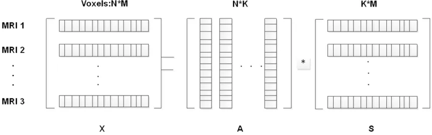
and mutually independent, and they are called the independent components of the observed data. ICA is typically modeled as Equation 2. X = A × S (2) The model is also demonstrated in Figure 2 in which X represents the observed multivariate data. Each row of X is resized from one image so that the number of columns is equal to the number of voxels in one image. X is decom-posed into mixing matrix A and source matrix S. Each row of A consists of all the independent components in one image, while each column of A is equivalent to one component of all imag-es. The source matrix S, which contains the information of voxels, can be used to recon-struct images.

Component analysis

We run the two-sample t-test the way we had conceived above, and we get the components that we need. The p-value we set in order to determine the choice of components was 0.05, which is a typical threshold value in a two-sam-ple t-test [61-63]. As mentioned before, matrix S holds the related information between voxels and components, so it can be used to realize the visualization of those components we have extracted. To do it, every row of source matrix was reshaped into a 3D image, scaled to the

unit standard deviation, and fit in a threshold at

|z| > 3.0. Then, the images of the components that we have chosen were overlaid on the nor-malized template image [64]. We could also

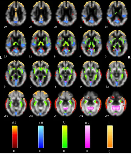
Figure 3. Independent components discovered after ICA. Different colors represent different sources. Red, compo-nent 1; blue, compocompo-nent 2; green, compocompo-nent 4; pink, compocompo-nent 11; orange, compocompo-nent 14.

components from the MNI coordinate system to the coordinates of the standard space of Talairach and Tournoux [57]. The trans-formed coordinates were then inputted into

the TalairachClient, a Java application for find -ing individual and batch labels, which was creat- ed and developed by Jack Lancaster and Pet- er Fox at the Research Imaging Center at the University of Texas Health Science Center, San

Antonio, which is available at http://www.talai-rach.org/. The output of the TalairachClient displayed summarized labels of the compo-nents we needed.

Classification

To perform classification, we first needed to

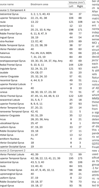
train-Table 3. Talairach labels for regions of significant sources (AD-HC)

Source name Brodmann area Volume (mm3)

Left Right Source 1: Component 4

Postcentral Gyrus 3, 2, 1, 5, 40, 43 54 37 Superior Temporal Gyrus 22, 21, 41, 38 106 88

Insula 13, 22 121 108

Rectal Gyrus 11 12 13

Sub-Gyral 20, 21, 10, 6, Hip 198 171 Middle Frontal Gyrus 6, 11, 8, 47, 9 69 77 Lingual Gyrus 18, 19 44 54

Extra-Nuclear 13, CC, AC 105 89

Middle Temporal Gyrus 21, 22, 38, 39 38 57

Inferior Parietal Lobule 40 69 60

Thalamus Pul, AN, VLN, MDN 55 66

Precuneus 7, 31, 23, 19 84 49

Parahippocampal Gyrus 19, 30, 35, 34, 37, Hip, Amy 40 69 Medial Frontal Gyrus 9, 10, 6, 11 144 129 Cingulate Gyrus 32, 24, 31, 23 121 93

Caudate CH, CB, CT 15 20

Anterior Cingulate 25, 32, 24, 10 57 61

Precentral Gyrus 4, 44, 6, 9 49 51

Superior Parietal Lobule 7 14 13

Supramarginal Gyrus 40 8 10

Cuneus 18, 30, 19, 17, 23, 30 73 51

Inferior Frontal Gyrus 47, 45, 11, 44, 46, 9, 13 122 120

Paracentral Lobule 31, 5, 6, 7 25 18

Superior Frontal Gyrus 8, 9, 6, 11 87 93 Inferior Temporal Gyrus 37, 20, 21 20 14 Transverse Temporal Gyrus 42, 41 11 5

Posterior Cingulate 30, 31, 29 35 12

Uncus 28, 20, 36, Amy 8 21

Subcallosal Gyrus 25, 47 8 1 Fusiform Gyrus 37, 19, 20 33 27 Middle Occipital Gyrus 19, 18 17 11 Orbital Gyrus 11, 47 13 12

Lentiform Nucleus Pu 4 15

Inferior Occipital Gyrus 18 8 3 Superior Occipital Gyrus 19 4 3 Source 2: Component 2

Inferior Parietal Lobule 40, 39 72 99

Superior Temporal Gyrus 42, 38, 22, 13, 41, 21, 39 195 175 Postcentral Gyrus 43, 5, 3, 40 65 106

Insula 13, 40, 41 84 101

Inferior Frontal Gyrus 44, 47, 9, 45, 10, 11 58 88 Supramarginal Gyrus 40 29 21 Fusiform Gyrus 37, 19 8 22 Middle Occipital Gyrus 19, 18, 37 78 70 Lingual Gyrus 19, 18, 17 93 76

ing and testing. The num-ber of independent compo-nents was estimated, whi- ch is represented as N. After ICA, we obtained the mixing matrix A and source

matrix S. We figured since

we had achieved N differ-ent independdiffer-ent compo-nents, we had caught N independent source areas at the same time. Common sense dictates that AD and MCI patients suffer great- er atrophy of inner brain structures than do HCs [65-68]. As a result, we decided to count our sub-jects’ number of voxels in each source region, and each subject could obtain N different numbers of vo- xels in different regions. Naturally we get N colu- mns of attributes. We also noticed that each subject of ADNI received a variety of clinical examinations, which is how a value like MMSE was obtained. All these values (to some ex- tent) differentiate patients from HC, and they display

a significant evaluation

pr-incipal in examining and determining the degree of dementia and the duration

of disease [69, 70]. Given

this consideration, we ex- panded the attribute mat- rix with another three col-umns of attributes: MMSE,

GDTOTAL and HMSCORE.

Finally, we constructed a new attribute matrix to be used in the following

clas-sification and assigned 1

as the label value for one group’s components and -1 for the other [71]. In con-sidering the situation that attributes in greater nume- ric ranges may dominate

the classification, we

Precuneus 7, 31, 19, 23 136 104 Cingulate Gyrus 31, 24, 32, 23 59 33

Extra-Nuclear CC 12 24

Posterior Cingulate 30, 31, 29, 23 58 53

Sub-Gyral 21, Hip, CC 38 53

Cuneus 17, 23, 7, 19, 18 147 126

Middle Temporal Gyrus 21, 39, 37, 22, 38, 19 111 194

Superior Parietal Lobule 7 19 19

Precentral Gyrus 4, 6, 9, 44, 43 95 135

Paracentral Lobule 31, 6, 5 17 10

Angular Gyrus 39 12 19

Transverse Temporal Gyrus 42, 41 24 27 Inferior Temporal Gyrus 20, 37, 19 11 16

Anterior Cingulate 32, 24, 25, CC 29 15

Middle Frontal Gyrus 11, 6, 9, 10, 8, 46 51 62 Parahippocampal Gyrus 28, 36, 35, 19, 34, 30, 27, 37 58 61 Superior Occipital Gyrus 19 11 1 Inferior Occipital Gyrus 18, 19 20 8

Uncus 36, 28, 34, 20 5 12

Medial Frontal Gyrus 9, 10, 6, 32, 25, 11 21 35 Superior Frontal Gyrus 10, 8, 6 4 10 Subcallosal Gyrus 34, 25 5 4

Thalamus Pul 2 4

Rectal Gyrus 11 1 3

Lentiform Nucleus Pu 0 2

Source 3: Component 14

Insula 13 66 67

Middle Temporal Gyrus 39, 20, 38, 21, 19 128 127 Inferior Temporal Gyrus 20, 21, 37 32 30

Precuneus 7, 31, 39, 31 34 39

Cingulate Gyrus 24, 23, 31, 32 155 135 Middle Frontal Gyrus 8, 10, 47, 9, 46, 11 298 278 Superior Frontal Gyrus 10, 11, 8, 9 232 259 Medial Frontal Gyrus 9, 10, 25, 11, 6, 25 126 115 Middle Occipital Gyrus 19, 18, 37 30 50 Parahippocampal Gyrus 34, 35, 28, 36, 37, Amy, Hip 48 32 Superior Temporal Gyrus 22, 38, 39, 13 158 182 Precentral Gyrus 6, 4, 9, 44, 13 93 97

Cuneus 19, 18, 17, 23, 30 19 10

Inferior Frontal Gyrus 47, 45, 46, 10, 44, 13, 11, 9 166 138 Sub-Gyral 6, 20, 7, CC 72 86

Extra-Nuclear 13, CC, OT 48 45

Posterior Cingulate 30, 31, 29, 23 35 35

Uncus 36, 28, 34, Amy 40 30

Paracentral Lobule 4, 31, 6 9 4

Orbital Gyrus 11, 47 14 11

Inferior Parietal Lobule 40, 7 58 56

Anterior Cingulate 32, 33, 24, 25, 10 66 67

Lentiform Nucleus Pu 8 15

result, the training matrix

was comprised of 50% of

the samples for the follow-ing processfollow-ing. Then we

used the other 50% of the

attribute matrix as our

test-ing matrix to find out the

effectiveness of the model we had generated from the training step. Here, we ca- lled on another Matlab

tool-box LIBSVM [34, 72],

de-veloped by Chih-Jen Lin of the National Taiwan Uni- versity for help. Two

impor-tant functions of this SVM

toolbox are the use of tra- ining data to generate a model and the use of the outcome model to predict the class-belonging of the testing data.

Results

ICA results

We first compared the

ima-ges between group AD and group HC, and then we compared the images be- tween group MCI and gr- oup HC in the same way. The results are explained below.

AD vs. HC

The number of indepen- dent components analyz- ed under the previous es- timation was 17. After that, the two-sample t-test was used to detect those sig-

nificant components, and

resulted in six independent components (out of the 17 components) being tested to show a p-value less th- an 0.05. Then, one compo-nent that implied obvious unimportant border infor-mation was excluded, and

the coordinates of the five

Superior Parietal Lobule 7 9 21 Transverse Temporal Gyrus 42, 41 6 18 Supramarginal Gyrus 40 6 20

Thalamus MDN, AN, Pul 11 11

Postcentral Gyrus 2, 3, 43, 40, 5, 1, 7, 4 89 65

Rectal Gyrus 11 23 10

Fusiform Gyrus 20, 19, 37 21 20

Angular Gyrus 39 10 14

Lingual Gyrus 18, 17 7 12 Superior Occipital Gyrus 19 7 6 Inferior Occipital Gyrus 18, 17 5 14

Subcallosal Gyrus 25 2 2

Caudate CH 4 1

Source 4: Component 11

Thalamus Pul, VPLN, MDN, VPLN, VLN, MB 32 37 Superior Temporal Gyrus 38, 22, 42 15 50

Precuneus 7, 23, 31, 39 40 20

Precentral Gyrus 4, 6, 44, 3 54 72

Orbital Gyrus 11, 47 0 5

Middle Temporal Gyrus 39, 37, 22, 38, 21, 20 36 57 Medial Frontal Gyrus 9, 11, 10, 6, 8, 25 29 33 Postcentral Gyrus 3, 43, 4, 5, 40, 2, 1, 7 43 67

Cuneus 18, 30, 19, 17, 7 47 47

Middle Frontal Gyrus 9, 6, 11, 8 22 33

Lentiform Nucleus Pu 5 5

Posterior Cingulate 31, 23, 30 29 13

Cingulate Gyrus 31, 24 35 14

Extra-Nuclear 13 36 44

Superior Frontal Gyrus 11, 9, 6, 8, 10 16 30

Inferior Parietal Lobule 40 25 37

Inferior Frontal Gyrus 47, 11, 45, 44, 9 29 45

Paracentral Lobule 31, 6, 5 7 6

Middle Occipital Gyrus 18 27 24

Uncus 20, 28, Amy 17 17

Lingual Gyrus 18, 19, 17 42 29

Anterior Cingulate 32, 24, 25 18 23

Parahippocampal Gyrus 36, 35, 34, Amy 30 31

Insula 13 8 57

Fusiform Gyrus 20 9 6

Inferior Temporal Gyrus 20, 21, 37 3 10

Caudate CH 2 3

Inferior Occipital Gyrus 19, 18 10 8

Superior Parietal Lobule 7 2 3

Subcallosal Gyrus 47 1 1

Supramarginal Gyrus 40 4 3 Source 5: Component 1

Middle Occipital Gyrus 19, 18, 37 67 88

Superior Frontal Gyrus 11, 10, 6, 9, 8 51 73 Medial Frontal Gyrus 25, 6, 10, 32, 8, 9 36 36

re transformed and their Talairach labels summari- zed. Also, we made the vi-

sualization of the five

av-ailable components, com-ponent 1, comcom-ponent 2, component 4, component 11 and component 14, as is shown in Figure 3. Their

p-values can be listed as 1.39 × 10-8_{, 2.24 × 10}-6_, 0.0024, 0.012, 0.017, re- spectively, so we can

rear-range the five components

in ascending order by their

p-values. As a result, we

had five sources represent

-ing five different areas that significantly decrease in

the gray matter of AD pa- tients’ images when com-pared to HCs.

The detailed Talairach la-

bels of these five sources

are listed in Table 3 in ord- er of increasing p values (1.39 × 10-8_{, 2.24 × 10}-6_, 0.0024, 0.012, 0.017). The areas involved in each so- urce with the correspond-ing Brodmann area were

arranged in the first two

columns. The volumes, in cubic millimeter, of the tar-get areas in the left cere-brum and right cerecere-brum were also displayed in the right two columns.

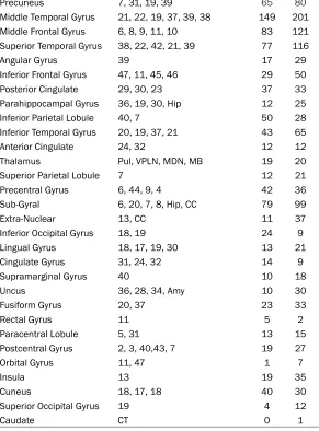
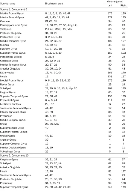
MCI vs. HC

Using the MIC criteria, the estimated independent co-mponents were found to be 11. From these 11 compo-nents, components 5 and

10 were two significant

Precuneus 7, 31, 19, 39 65 80 Middle Temporal Gyrus 21, 22, 19, 37, 39, 38 149 201 Middle Frontal Gyrus 6, 8, 9, 11, 10 83 121 Superior Temporal Gyrus 38, 22, 42, 21, 39 77 116

Angular Gyrus 39 17 29

Inferior Frontal Gyrus 47, 11, 45, 46 29 50

Posterior Cingulate 29, 30, 23 37 33

Parahippocampal Gyrus 36, 19, 30, Hip 12 25

Inferior Parietal Lobule 40, 7 50 28

Inferior Temporal Gyrus 20, 19, 37, 21 43 65

Anterior Cingulate 24, 32 12 12

Thalamus Pul, VPLN, MDN, MB 19 20

Superior Parietal Lobule 7 12 21

Precentral Gyrus 6, 44, 9, 4 42 36 Sub-Gyral 6, 20, 7, 8, Hip, CC 79 99

Extra-Nuclear 13, CC 11 37

Inferior Occipital Gyrus 18, 19 24 9 Lingual Gyrus 18, 17, 19, 30 13 21 Cingulate Gyrus 31, 24, 32 14 9 Supramarginal Gyrus 40 10 18

Uncus 36, 28, 34, Amy 10 30

Fusiform Gyrus 20, 37 23 33

Rectal Gyrus 11 5 2

Paracentral Lobule 5, 31 13 15

Postcentral Gyrus 2, 3, 40,43, 7 19 27

Orbital Gyrus 11, 47 1 7

Insula 13 19 35

Cuneus 18, 17, 18 40 30

Superior Occipital Gyrus 19 4 12

Caudate CT 0 1

Abbreviations: AC = Anterior Commissure, Amy = Amygdala, AN = Anterior Nucleus, CB = Caudate Body, CC = Corpus Callusum, CH = Caudate Head, CT = Caudate Tail, Hyp

= Hpyothalamus, Hip = Hippocampus, LGP = Lateral Globus Pallidus, MB = Mamillary

Body, MDN = Medial Dorsal Nucleus, OT = Optic Tract, Pu = Putamen, Pul = pulvinar,

VLN = Ventral Lateral Nucleus, VPLN = Ventral Posterior Lateral Nucleus.

averaged values of accura-cy, sensitivity, and speci-

ficity. The number of true

positives (TP) denote the number of patients

correct-ly classified; TN, the num -ber of true negatives; FP, the number of false po- sitives; and FN, the numb- er of false negatives, with

the classification accura-cy defined as accuraaccura-cy =

(TP+TN)/(TP+FP+TN+FN), in

which the specificity is de-fined as sensitivity = TP/(TP

+FP), and the sensitivity as

specificity = TN/(TN+FN).

Discussion

Why ICA?

Our summarized results

are as follows: first, the vol -ume of gray matter in bo- th MCI subjects and AD pa- tients’ brains had declined, with the difference being that the AD patients’ gr- oup had a greater decline. Second, the Talairach la- bels anatomically implied that (compared to healthy people) MCI subjects suf-fered gray matter loss ma- inly in the cerebellar tonsil, culmen, tuber, declive, infe-rior semi-lunar lobule, uvu- la and fusiform gyrus, whi- le AD patients also lost gray Figure 4, and the Talairach label of each is

summarized in Table 4.

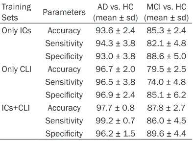
Classification results

Since we randomly chose 50% of the

sam-ples for training, a different dataset consist- ing of different subjects may result in diffe- rent outcomes. To handle this, we carried out

the classification multiple times so that we

could get the statistically averaged value. Figure 5 displays the results of our 100 analy-ses in two sets of comparisons, and in Table 5, the part of independent components and clinical measurements (ICs+CLI) display the

matter in areas like the parahippocampal gyrus, posterior cingulate, temporal gyrus, and so on. Our results were consistent using our research approaches, but compared to previ-ous studies. One difference experienced was that the lost gray matter in MCI that is, to so- me extent, the preliminary stage of AD. Third, since we have achieved the detailed Talairach labels of the declined areas, it is possible for related experts to do more in-depth research

in the field.

We have made clear that the clinical exami-

nation value like MMSE is a significant

Figure 4. Sources discovered between groups MCI and HC. Red, component 5; blue, component 10.

questions are: how can those results express the effect of ICA? Is there a possibility that it is those clinical examination gains that have

highlighted our classification accuracy? The fol -lowing discussion shows our results. We took off the columns of voxel numbers from the at- tribute data matrix and re-constructed it wi-

th just three columns: MMSE, GDTOTAL, and

HMSCORE [69, 70]. Labeled as it had been before, the training matrix was built by

random-ly picking 50% of the rows of attributes from

the new data matrix. A new model came out after training these data, and then the whole matrix was entered into the predictive function

of LIBSVM. Similarly, to get rid of the exception

-al case, depending on single specific predic -tion, we summed up 100 results and statisti-cally averaged the value of all these 100 cases in Figure 6. This allowed us to come up with the

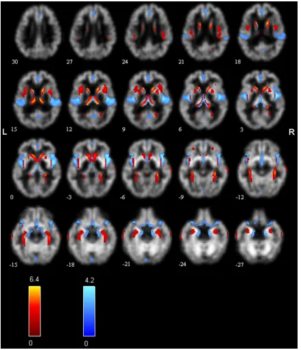
Table 4. Talairach labels for regions of significant sources (MCI-HC)

Source name Brodmann area Volume (cmm)

Left Right Source 1: Component 5

Middle Frontal Gyrus 8, 11, 6, 9, 10, 46, 47 176 139 Inferior Frontal Gyrus 47, 9, 45, 11, 13, 44 124 115

Caudate CT, CB, CH 34 40

Parahippocampal Gyrus 19, 30, 20, 37, 36, Amy, Hip 63 79

Thalamus Pul, AN, MDN, LPN, VAN 63 63

Posterior Cingulate 31, 30, 29 24 25

Postcentral Gyrus 3, 2, 40, 5, 43 63 76 Middle Temporal Gyrus 21, 22, 39, 37 102 127

Cuneus 17, 30, 19 35 51

Fusiform Gyrus 19, 37, 20, 18 75 63

Superior Frontal Gyrus 6, 11, 9, 8, 10 169 123

Paracentral Lobule 5, 31, 6 24 28

Cingulate Gyrus 24, 32, 9, 31 38 30

Inferior Temporal Gyrus 20, 37, 21 50 38

Anterior Cingulate 32, 25, 10, 24 51 48

Extra-Nuclear 13, AC, CC, OT 165 140

Insula 13 138 137

Medial Frontal Gyrus 9, 8, 11, 10, 32, 6, 25 176 199

Rectal Gyrus 11 23 19

Sub-Gyral 21, 20, 6, 10, 13, 8, Hip, CC 264 185

Lingual Gyrus 18, 17, 19 63 37

Superior Temporal Gyrus 22, 38, 42 133 135

Precentral Gyrus 6, 4, 9, 44 112 95

Lentiform Nucleus Pu, LGP 17 27

Transverse Temporal Gyrus 41, 42 12 14

Inferior Parietal Lobule 40, 39 86 93

Precuneus 31, 7, 19 51 55

Middle Occipital Gyrus 19, 37, 18 39 28

Uncus 28, 36, Amy 8 20

Supramarginal Gyrus 40 2 16

Superior Parietal Lobule 7 15 12

Orbital Gyrus 47, 11 19 18

Angular Gyrus 39 4 3

Superior Occipital Gyrus 19 1 4

Inferior Occipital Gyrus 18, 19 6 11

Subcallosal Gyrus 25 5 8

Source 2: Component 10

Cingulate Gyrus 32, 31, 24 61 37

Sub-Gyral 21, 13, CC, Hip 67 78

Anterior Cingulate 32, 25, 24, 10 61 55

Insula 13, 40 81 117

Transverse Temporal Gyrus 41, 42 24 29

Posterior Cingulate 23, 31, 30, 29 53 44

Precuneus 31, 7, 23, 19 99 100

Parahippocampal Gyrus 34, 28, 30, 35, 36, 27, 35, 19, Hip, Amy 112 72

Paracentral Lobule 31, 6, 5, 31 18 17

Cuneus 19, 17, 18, 30, 7, 23 101 81

Middle Frontal Gyrus 9, 6, 10, 46, 11, 8 65 61

Fusiform Gyrus 19, 18, 20, 37 29 33

Inferior Frontal Gyrus 47, 9, 44, 47,46, 45, 11 174 122 Middle Temporal Gyrus 22, 21, 19, 39, 38 112 132

Extra-Nuclear CC, AC 60 50

Precentral Gyrus 6, 4, 43, 44, 9 86 97 Superior Frontal Gyrus 10, 8, 11 52 43 Postcentral Gyrus 3, 40, 2, 43, 5 97 78 Medial Frontal Gyrus 9, 10, 6, 11, 8, 25 145 79 Middle Occipital Gyrus 18, 19, 37 19 30

Uncus 34, 28, 36, 20, 36 37 15

Lingual Gyrus 17, 18, 19 70 59

Inferior Parietal Lobule 40 75 50

Thalamus Pul, MDN, LPN, VAN 24 23

Inferior Temporal Gyrus 20, 37 11 17

Subcallosal Gyrus 25, 34 7 6

Caudate CH, CB 16 23

Supramarginal Gyrus 40 32 7

Rectal Gyrus 11 24 21

Orbital Gyrus 11, 47 22 13

Inferior Occipital Gyrus 17, 18 8 25

Lentiform Nucleus Pu, LGP 1 5

Superior Parietal Lobule 7 2 6

Superior Occipital Gyrus 19 1 6

Angular Gyrus 39 1 6

a similarly high level, with sensitivity at almost an identical level. The averaged accuracy,

sen-sitivity, and specificity after testing under this circumstance turned out to be 96.7%, 96.5%, and 96.9% for group AD, and 79.5%, 74.0%, 85.1% for group MCI using only CLI, compared to 97.7%, 99.2%, 96.2% for groups AD and HC, and 87.8%, 86.0%, 89.6% for groups MCI

and HC using both ICs and CLI. The latter’s re-

lative poorer accuracy implied that classifica -tion relying on the clinical examina-tion values are unilateral and not all-inclusive. The ICA

section of our trial provided better classifica -tion capabilities. The averaged results of all those 100 experiments can be found in Table 5 in which classifications between AD and HC,

as well as MCI and HC, were both displayed. According to a different training set, Table 5 was divided into three parts. In the Only ICs

part, we showed the classification accuracy

using only the numbers of voxels in each

com-ponent region based on ICA, while in the sec-ond part the Only CLI were results of merely clinical measurements. The last one, the ICs+CLI, resulted from a combination of both feature sources. In Figure 7 we displayed the accuracy values of these three parts for better visualization.

We have chosen MIC as our independent component estimation criterion. To testify its superiority, we also used AIC and MDL to esti-mate the number of independent components between group AD and group HC, and it turn- ed out to be 34 of AIC and 17 of MDL. As MDL shared the same independent component

number, the significant components by the

Figure 5. The classification accuracy, sensitivity, and specificity of 100 tests.

Table 5. Classification accuracy of AD or MCI

from healthy controls Training

Sets Parameters (mean ± sd)AD vs. HC (mean ± sd)MCI vs. HC Only ICs Accuracy 93.6 ± 2.4 85.3 ± 2.4

Sensitivity 94.3 ± 3.8 82.1 ± 4.8 Specificity 93.0 ± 3.8 88.6 ± 5.0 Only CLI Accuracy 96.7 ± 2.0 79.5 ± 2.5 Sensitivity 96.5 ± 3.8 74.0 ± 4.8 Specificity 96.9 ± 2.4 85.1 ± 6.2 ICs+CLI Accuracy 97.7 ± 0.8 87.8 ± 2.7 Sensitivity 99.2 ± 0.7 86.0 ± 4.5 Specificity 96.2 ± 1.5 89.6 ± 4.4

23, 24, 25, 26, 27, 28, 29 and 33 showed mo- re of a difference between the two engaged groups. To get a clear visualization, here, we showed components 4, 5, 20, 24, and 33,

which corresponded to the smallest five p

val-ues compared to other components in Figure 8. Therefore, it was not hard to find that the

resulting area was mostly compatible in the MIC result and in the AIC result. What we co- uld draw out was that the AIC result was sug-gestive of more artifacts, such as showing sharp edges (e.g. component 2 with larger p

value) appearing mainly in regions that do not contain gray matter (e.g. white matter or ven-tricles), and so on.

In using structural MRI images for

classifica-tion between AD, MCI and HC, researchers like Fan [34, 35, 73] extracted voxel-wise tissue

probability as features for classification.

Cor-tical thickness [74-76] was another source of features and was used in certain research. Hippocampal volumes of subjects were

calcu-lated and applied into classification as a fea

-ture by researchers like Gerardin [77, 78]. It

Figure 6. The classification accuracy, sensitivity, and specificity of 100 tests using only clinical measures.

ons such as the hippocampus, amygdala, ento-rhinal cortex, uncus, temporal pole and para-hippocampal regions are the top regions that are selected and closely interrelated to AD [79-81]. However, in this research, each only used partial information of these regions and therefore it could be improved upon. Besides, with sMRI and other modalities such as PET, the CSF also contains complementary infor- mation for the diagnosis of AD. Reports of combining biomarkers from different modali-ties have been released. Among them, there were some practices concatenating all fea- tures from different modalities into a larger feature matrix [82, 83]. Researchers like Ye and Zhang [24, 84] further developed this method by using a kernel combination method to construct biomarkers from different

modali-ties into a unified feature matrix. We can see

that these recent ways, to a certain extent, ta-

ke into better consideration features that co- uld differentiate groups by combining more information of different modalities to reveal better results. The method we propose here considers almost all of the interested regions mentioned above that can be discovered from the table by way of ICA. Moreover, integrated with commonly used clinical measures, this method showed more satisfactory results. A future consideration is to use amethod that can explore the values of voxels and their num-bers in those interested regions, and modify the way we comb values to extract both voxels and clinical measures.

Conclusion

In our study, we aimed to find innovative and

Figure 7. Comparison among three classifications using different feature matrix. Only ICs: classification accuracy using only the numbers of voxels in each component region based on ICA; Only CLI: only clinical measurements were used to construct feature matrix; ICs+CLI: accuracy came out of the combination of both feature sources.

HC subjects. To reach this goal, we set up our experimental process using the following ste-

ps: first, the pre-processing stage involved a

set of conducts being applied to the subject dataset in order to make sure that all the data in the following steps met the IID requirement. Then we extracted the biological characters using ICA (or we can call this analyzing me-

thod SBM). Compared with VBM, it is a

multi-covariate approach that takes the spatial infor-mation among coherent voxels into consider-ation. Before we actually executed ICA, we compar- ed several common ITC and chose MIC to per-form the independent components estimation.

After all these, we analyzed the specific

com-ponents that had been drawn out from the

dataset and obtained visualization and

gath-ered the Talairach labels of all the significant

sources. Lastly, we extracted features that

significantly differentiated groups and classi

-fied them. The results we obtained reveal that

AD patients’ brains change mostly in the are- as of the hippocampus, amygdala, and so on, as some research has already revealed. MCI subjects also experience brain tissue loss, but the volume of gray matter lost is far less, indi-cating that MCI is, to some extent, the previous stage of AD. Since we are not professionals in psychiatry, the conclusions we can draw are

limited. What we find gratifying is that our

Figure 8. Components 4, 5, 20, 24, and 33 using AIC to estimate the number of independent components.

helpful. ICA was brought into morphometry analysis, making it multivariate to better con-sider spatial information among the neighbor-ing voxels clustered in one source. MIC applied in our independent components estimation before ICA showed better results in terms of the

number of independent components.The final classification revealed that ICA was a poten -tially useful approach to analyze MRIs and to extract the features we needed.

Acknowledgements

The authors would like to express their grati-tude for the support from the Shanghai Ma-

ritime University (Grant No. 20090175 to WY), and for the NIH grant (R01 AG056614 to XH).

tes of Health Grant U01 AG024904) and DOD

ADNI (Department of Defense awardnumber W81XWH-12-2-0012). ADNI is funded by the National Institute on Aging, the National Insti- tute of Biomedical Imaging and Bioengineer- ing, and through generous contributions from

the following: AbbVie, Alzheimer’s Association;

Alzheimer’s Drug Discovery Foundation; Ara- clon Biotech; Bio Clinica, Inc.; Biogen; Bristol-Myers Squibb Company; CereSpir, Inc.; Cog- state; Eisai Inc.; Elan Pharmaceuticals, Inc.; Eli Lilly andCompany; EuroImmun; F. Hoffmann-La

Roche Ltd and its affiliated company Genen-tech, Inc.; Fujirebio; GE Health care; IXICO Ltd.;

Janssen Alzheimer Immunotherapy Research & Development, LLC.; Johnson & Johnson Phar- maceutical Research & Development LLC.; Lumosity; Lundbeck; Merck & Co., Inc.; Me- soScale Diagnostics, LLC.; NeuroRx Research; Neurotrack Technologies; Novartis Pharma-

ceuticals Corporation; Pfizer Inc.; Piramal

Ima-ging; Servier; Takeda Pharmaceutical Com- pany; and Transition Therapeutics. The Ca- nadian Institutes of Health Research is provid-ing funds to support ADNI clinical sitesin Canada. Private sector contributions are fa- cilitated by the Foundation for the National Institutes of Health (www.fnih.org). The gran- tee organization is the Northern California In- stitute for Research and Education, and the study is coordinated by the Alzheimer’s The- rapeutic Research Institute at the University of Southern California. ADNI data are dissemi-nated by the Laboratory for Neuro Imaging at the University of Southern California.

Disclosure of conflict of interest None.

Address correspondence to: Dr. Xudong Huang, Neurochemistry Laboratory, Department of Psy- chiatry, Massachusetts General Hospital and Har-vard Medical School, 149 13th _{Street, Charlestown,} MA 02129, USA. Tel: 617-724-9778; E-mail: Huang. [email protected]

References

[1] Braak H and Braak E. [Morphological changes in the human cerebral cortex in dementia]. J Hirnforsch 1991; 32: 277-282.

[2] Small GW, Ercoli LM, Silverman DH, Huang SC, Komo S, Bookheimer SY, Lavretsky H, Miller K, Siddarth P, Rasgon NL, Mazziotta JC, Saxena S, Wu HM, Mega MS, Cummings JL, Saunders

AM, Pericak-Vance MA, Roses AD, Barrio JR and Phelps ME. Cerebral metabolic and cogni-tive decline in persons at genetic risk for Al-zheimer’s disease. Proc Natl Acad Sci U S A 2000; 97: 6037-42.

[3] Jack CR Jr, Shiung MM, Gunter JL, O’Brien PC, Weigand SD, Knopman DS, Boeve BF, Ivnik RJ, Smith GE, Cha RH, Tangalos EG, Petersen RC. Comparison of different MRI brain atrophy rate measures with clinical disease progression in AD. Neurology 2004; 62: 591-600.

[4] Dickerson BC, Salat DH, Greve DN, Chua EF, Rand-Giovannetti E, Rentz DM, Bertram L, Mul -lin K, Tanzi RE, Blacker D, Albert MS and Sper-ling RA. Increased hippocampal activation in mild cognitive impairment compared to normal aging and AD. Neurology 2005; 65: 404-411. [5] Killiany RJ, Gomez-Isla T, Moss M, Kikinis R,

Sandor T, Jolesz F, Tanzi R, Jones K, Hyman BT and Albert MS. Use of structural magnetic res-onance imaging to predict who will get Al-zheimer’s disease. Ann Neurol 2000; 47: 430-439.

[6] Greicius MD, Srivastava G, Reiss AL and Me -non V. Default-mode network activity distin -guishes Alzheimer’s disease from healthy ag-ing: evidence from functional MRI. Proc Natl Acad Sci U S A 2004; 101: 4637-4642. [7] Sperling R. Functional MRI studies of

associa-tive encoding in normal aging, mild cogniassocia-tive impairment, and Alzheimer’s disease. Ann N Y Acad Sci 2007; 1097: 146-155.

[8] Frisoni GB, Fox NC, Jack CR, Scheltens P and Thompson PM. The clinical use of structural MRI in Alzheimer disease. Nat Rev Neurol 2010; 6: 67-77.

[9] Cavedo E, Lista S, Khachaturian Z, Aisen P, Amouyel P, Herholz K, Jack C, Sperling R, Cum-mings J, Blennow K, O’Bryant S, Frisoni G, Kha -chaturian A, Kivipelto M, Klunk W, Broich K, Andrieu S, de Schotten MT, Mangin J, Lam-mertsma A, Johnson K, Teipel S, Drzezga A, Bokde A, Colliot O, Bakardjian H, Zetterberg H, Dubois B, Vellas B, Schneider L and Hampel H. The road ahead to cure Alzheimer’s disease: development of biological markers and neuro-imaging methods for prevention trials across all stages and target populations. J Prev Al-zheimers Dis 2014; 1: 181-202.

[10] Bangen KJ, Restom K, Liu TT, Wierenga CE, Jak AJ, Salmon DP and Bondi MW. Assessment of Alzheimer’s disease risk with functional mag-netic resonance imaging: an arterial spin label-ing study. J Alzheimers Dis 2012; 31: S59-74. [11] Foster NL, Chase TN, Fedio P, Patronas NJ,

[12] Duara R, Grady C, Haxby J, Sundaram M, Cutler NR, Heston L, Moore A, Schlageter N, Larson S and Rapoport SI. Positron emission tomogra-phy in Alzheimer’s disease. Neurology 1986; 36: 879-87.

[13] Silverman DH, Small GW, Chang CY, Lu CS, Kung De Aburto MA, Chen W, Czernin J, Rapo-port SI, Pietrini P, Alexander GE, Schapiro MB, Jagust WJ, Hoffman JM, Welsh-Bohmer KA, Alavi A, Clark CM, Salmon E, de Leon MJ, Miel-ke R, Cummings JL, Kowell AP, Gambhir SS, Hoh CK, Phelps ME. Positron emission tomog-raphy in evaluation of dementia-regional brain metabolism and long-term outcome. JAMA 2001; 286: 2120-7.

[14] Marcus C, Mena E and Subramaniam RM. Brain PET in the diagnosis of Alzheimer’s dis-ease. Clin Nucl Med 2014; 39: e413-426. [15] Jack CR Jr, Petersen RC, O’Brien PC and

Tanga-los EG. MR-based hippocampal volumetry in the diagnosis of Alzheimer’s disease. Neurolo-gy 1992; 42: 183-188.

[16] Nestor PJ, Fryer TD, Smielewski P and Hodges JR. Limbic hypometabolism in Alzheimer’s dis-ease and mild cognitive impairment. Ann Neu-rol 2003; 54: 343-351.

[17] Greicius MD, Srivastava G, Reiss AL and Me -non V. Default-mode network activity distin -guishes Alzheimer’s disease from healthy ag-ing: evidence from functional MRI. Proc Natl Acad Sci U S A 2004; 101: 4637-4642. [18] Desikan RS, Sonne F, Fischl B, Quinn BT,

Dick-erson BC, Blacker D, Buckner RL, Dale AM, Ma-guire RP, Hyman BT, Albert MS and Killiany RJ. An automated labeling system for subdividing the human cerebral cortex on MRI scans into gyral based regions of interest. Neuroimage 2006; 31: 968-980.

[19] Marshall GA, Lorius N, Locascio JJ, Hyman BT, Rentz DM, Johnson KA and Sperling RA. Re-gional cortical thinning and cerebrospinal bio-markers predict worsening daily functioning across the Alzheimer disease spectrum. J Al-zheimers Dis 2014; 41: 719-728.

[20] Donovan NJ, Wadsworth LP, Lorius N, Locascio JJ, Rentz DM, Johnson KA, Sperling RA and Marshall GA. Regional cortical thinning pre -dicts worsening apathy and hallucinations across the Alzheimer’s disease spectrum. Am J Geriatr Psychiatry 2014; 22: 1168-1179. [21] Chupin M, Gerardin E, Cuingnet R, Boutet C,

Lemieux L, Lehericy S, Benali H, Garnero L and Colliot O. Fully automatic hippocampus seg-mentation and classification in Alzheimer’s disease and mild cognitive impairment applied on data from ADNI. Hippocampus 2009; 19: 579-587.

[22] Zhou L, Hartley R, Wang L, Lieby P and Barnes N. Identifying anatomical shape difference by

regularized discriminative direction. IEEE Trans Med Imaging 2009; 28: 937-50.

[23] Putcha D, Brickhouse M, O’Keefe K, Sullivan C, Rentz D, Marshall G, Dickerson B and Sperling R. Hippocampal hyperactivation associated with cortical thinning in Alzheimer’s disease signature regions in non-demented elderly adults. J Neurosci 2011; 31: 17680-17688. [24] Zhang D, Wang Y, Zhou L, Yuan H and Shen D.

Multimodal classification of Alzheimer’s dis -ease and mild cognitive impairment. Neuroim-age 2011; 55: 856-867.

[25] Ashburner J, Friston KJ. Voxel-based morphom -etry-the methods. NeuroImage 2000; 11: 805-821.

[26] Ashburner J and Friston KJ. Voxel-based mor -phometry-the methods. Neuroimage 2000; 11: 805-821.

[27] Hua X, Gutman B, Boyle CP, Rajagopalan P, Leow AD, Yanovsky I, Kumar AR, Toga AW, Jack CR Jr, Schuff N, Alexander GE, Chen K, Reiman EM, Weiner MW and Thompson PM. Accurate measurement of brain changes in longitudinal MRI scans using tensor-based morphometry. Neuroimage 2011; 57: 5-14.

[28] Hirata Y, Matsuda H, Nemoto K, Ohnishi T, Hirao K, Yamashita F, Asada T, Iwabuchi S and Samejima H. Voxel-based morphometry to dis -criminate early Alzheimer’s disease from con-trols. Neurosci Lett 2005; 382: 269-274. [29] Wang WY, Yu JT, Liu Y, Yin RH, Wang HF, Wang

J, Tan L, Radua J and Tan L. Voxel-based meta-analysis of grey matter changes in Alzheimer’s disease. Transl Neurodegener 2015; 4: 6. [30] Giesel FL, Thomann PA, Hahn HK and Wilkin

-son ID. Compari-son of manual direct and auto-mated indirect measurement of hippocampus using magnetic resonance imaging. Eur J Ra-diol 2008; 66: 268-273.

[31] Xu L, Groth KM, Pearlson G, Schretlen DJ and Calhoun VD. Source-based morphometry: the use of independent component analysis to identify gray matter differences with applica-tion to schizophrenia. Hum Brain Mapp 2009; 30: 711-724.

[32] Xu L, Pearlson G and Calhoun VD. Joint source based morphometry identifies linked gray and white matter group differences. Neuroimage 2009; 44: 777-789.

[33] Wax M and Kailath T. Detection of signals by information theoretic criteria. IEEE Transac-tions on Acoustics Speech & Signal Processing 1985; 33: 387-392.

[35] Kloppel S, Stonnington CM, Chu C, Draganski B, Scahill RI, Rohrer JD, Fox NC, Jack CR Jr, Ashburner J and Frackowiak RS. Automatic classification of MR scans in Alzheimer’s dis -ease. Brain 2008; 131: 681-689.

[36] Suykens JAK and Vandewalle J. Least squares support vector machine classifiers. Neural Pro -cessing Letters 1999; 9: 293-300.

[37] Cauwenberghs G and poggio T. Incremental and decremental support vector machine learning. Neural information Processing Sys-tems 2000; 13: 409-415.

[38] Zhang Y, Dong Z, Phillips P, Wang S, Ji G, Yang J and Yuan TF. Detection of subjects and brain regions related to Alzheimer’s disease using 3D MRI scans based on eigenbrain and ma-chine learning. Front Comput Neurosci 2015; 9: 66.

[39] Fung GM and Mangasarian OL. Multicategory proximal support vector machine classifiers. Machine Learning 2005; 59: 77-97.

[40] Jack CR Jr, Bernstein MA, Fox NC, Thompson P, Alexander G, Harvey D, Borowski B, Britson PJ, L Whitwell J, Ward C, Dale AM, Felmlee JP, Gunter JL, Hill DL, Killiany R, Schuff N, Fox-Bo -setti S, Lin C, Studholme C, DeCarli CS, Krueger G, Ward HA, Metzger GJ, Scott KT, Mallozzi R, Blezek D, Levy J, Debbins JP, Fleisher AS, Al-bert M, Green R, Bartzokis G, Glover G, Mugler J, Weiner MW. The Alzheimer’s disease neuro-imaging Initiative (ADNI): MRI methods. J Magn Reson Imaging 2008; 27: 685-691.

[41] Zhan L, Bernstein MA, Borowski B, Jack CR and Thompson PM. Evaluation of diffusion im-aging protocols for the Alzheimer’s disease neuroimaging initiative. IEEE International Symposium on Biomedical Imaging 2014; 710-713.

[42] Weiner MW, Veitch DP, Aisen PS, Beckett LA, Cairns NJ, Cedarbaum J, Green RC, Harvey D, Jack CR, Jagust W, Luthman J, Morris JC, Pe-tersen RC, Saykin AJ, Shaw L, Shen L, Schwarz A, Toga AW and Trojanowski JQ. 2014 update of the Alzheimer’s disease neuroimaging initia-tive: a review of papers published since its in-ception. Alzheimers Dement 2015; 11: e1-120.

[43] Kohannim O, Hua X, Hibar DP, Lee S, Chou YY, Toga AW, Jack CR, Weiner MW and Thompson PM. Boosting power for clinical trials using classifiers based on multiple biomarkers. Neu -robiol Aging 2010; 31: 1429-1442.

[44] Schafhitzel T, Rößler F, Weiskopf D and Ertl T. Simultaneous visualization of anatomical and functional 3D data by combining volume ren-dering and flow visualization. 2007.

[45] Schwarz G. Estimating the dimension of a model. Ann Statist 1978; 6: 461-464.

[46] AI H. A new look at the statistical model identi-fication. Automatic Control IEEE Transactions on 1974; 19: 716-723

[47] Wang G, Ding Q, Sun Y, He L and Sun X. Estima -tion of source infrared spectra profiles of ace -tylspiramycin active components from troches using kernel independent component analysis. Spectrochim Acta A Mol Biomol Spectrosc 2008; 70: 571-576.

[48] Williams DB. Comparison of AIC and MDL to the minimum probability of error criterion. Sta-tistical signal and array processing, 1992. Con-ference proceeding., IEEE Sixth SP Workshop on 1992; 114-117.

[49] Li YO, Adali T and Calhoun VD. Estimating the number of independent components for func-tional magnetic resonance Imaging data. Hu-man Brain Mapping 2007; 28: 1251-1266. [50] Wei X, Li YO, Li H, Adali T and Calhoun VD. On

ICA of complex-valued fMRI: advantages and order selection. 2008 IEEE International Con-ference on Acoustics, Speech and Signal Pro-cessing 2008; 529-532.

[51] Sekmen AS and Bingul Z. Comparison of algo-rithms for detection of the number of signal sources. Southeastcon 99 IEEE; 1999: 70-73. [52] Ashburner J. Computational anatomy with the SPM software. Magnetic Resonance Imaging 2009; 27: 1163-1174.

[53] Abel T, Morabia A and Kohlmann T. New name and new perspectives for the international journal of public health, formerly SPM. Int J Public Health 2007; 52: 1.

[54] Talairach J. Co-planar stereotaxic atlas of the human brain. Thieme Medical 1989.

[55] Calhoun V and Pekar J. When and where are components independent? On the applicability of spatial and temporal ICA to functional MRI data. NeuroImage 2000; 11: 682.

[56] Calhoun VD, Adali T, Hansen LK, Larsen J and Pekar J. ICA of functional MRI data: an over-view. International Workshop on Independent Component Analysis & Blind Signal Separation 2003; 281-288.

[57] Rachakonda S, Egolf E, Correa N and Calhoun V. Group ICA of fMRI Toolbox (GIFT) Manual. 2010.

[58] Adeli H, Ghosh-Dastidar S and Dadmehr N. Al -zheimer’s disease and models of computation: Imaging, classification, and neural models. J Alzheimers Dis 2005; 7: 187-199.

[59] Amari S. Natural gradient learning for over- and under-complete bases in ICA. Neural Computa-tion 1999; 11: 1875-1883.

[61] Calhoun V, Adali T and Pearlson G. Indepen -dent component analysis applied to fMRI data: a generative model for validating results. IEEE Signal Processing Society Workshop 2004; 37: 509-518.

[62] Calhoun V, Adali T, Pearlson G and Pekar J. A method for making group inferences using in-dependent component analysis of functional MRI data: exploring the visual system. Neuro-image 2001; 13: S88.

[63] Calhoun V, Adali T, Pearlson G and Pekar J. Group ICA of functional MRI data: separability, stationarity and inference. 2001.

[64] Rachakonda S, Egolf E and Calhoun V. Group ICA of fMRI toolbox (GIFT) walk through. 2010. [65] Apostolova LG, Dutton RA, Dinov ID, Hayashi KM, Toga AW, Cummings JL and Thompson PM. Conversion of mild cognitive impairment to Alzheimer disease predicted by hippocam-pal atrophy maps. Arch Neurol 2006; 63: 693-699.

[66] Beyer MK, Janvin CC, Larsen JP and Aarsland D. A magnetic resonance imaging study of pa-tients with Parkinson’s disease with mild cog-nitive impairment and dementia using voxel-based morphometry. J Neurol Neurosurg Psychiatry 2007; 78: 254-9.

[67] Apostolova LG and Thompson PM. Mapping progressive brain structural changes in early Alzheimer’s disease and mild cognitive impair-ment. Neuropsychologia 2008; 46: 1597-1612.

[68] Tarawneh R, Head D, Allison S, Buckles V, Fa -gan AM, Ladenson JH, Morris JC and Holtzman DM. Cerebrospinal fluid markers of neurode -generation and rates of brain atrophy in early Alzheimer disease. JAMA Neurol 2015; 72: 656-665.

[69] Solomon PR, Adams FA, Groccia ME, DeVeaux R, Growdon JH and Pendlebury WW. Correla -tional analysis of five commonly used mea -sures of mental status/functional abilities in patients with Alzheimer disease. Alzheimer Dis Assoc Disord 1999; 13: 147-50.

[70] Solomon TM, deBros GB, Budson AE, Mirkovic N, Murphy CA and Solomon PR. Correlational analysis of 5 commonly used measures of cog-nitive functioning and mental status. Am J Al-zheimers Dis Other Demen 2014; 29: 718-22. [71] Chang DJ, Zubal IG, Gottschalk C, Freeman J,

Necochea A, Stokking R, Studholme C, Corsi M, Spencer SS and Blumenfeld H. Statistical parametric mapping: a new approach to analy-sis of ictal SPECT scans in temporal lobe epi-lepsy compared to conventional difference im-aging. Society for Neuroscience Abstracts 2001; 27: 1464.

[72] Chang CC and Lin CJ. LIBSVM: a library for sup -port vector machines. ACM Transactions on

Intelligent Systems and Technology (TIST) 2011; 2: 27.

[73] Fan Y, Shen D, Gur RC, Gur RE, Davatzikos C. COMPARE: classification of morphological pat -terns using adaptive regional elements. IEEE Trans Med Imaging 2007; 26: 93-105.

[74] Desikan RS, Cabral HJ, Hess CP, Dillon WP, Glastonbury CM, Weiner MW, Schmansky NJ, Greve DN, Salat DH, Buckner RL, Fischl B; Al -zheimer’s Disease Neuroimaging Initiative. Au-tomated MRI measures identify individuals with mild cognitive impairment and Alzheim-er’s disease. Brain 2009; 132: 2048-2057. [75] Lerch JP, Pruessner J, Zijdenbos AP, Collins DL,

Teipel SJ, Hampel H, Evans AC. Automated cor-tical thickness measurements from MRI can accurately separate Alzheimer’s patients from normal elderly controls. Neurobiol Aging 2008; 29: 23-30.

[76] Querbes O, Aubry F, Pariente J, Lotterie JA, Dé-monet JF, Duret V, Puel M, Berry I, Fort JC, Cel -sis P; Alzheimer’s Disease Neuroimaging Initia-tive. Early diagnosis of Alzheimer’s disease using cortical thickness: impact of cognitive reserve. Brain 2009; 132: 2036-2047. [77] Gerardin E, Chetelat G, Chupin M, Cuingnet R,

Desgranges B, Kim HS, Niethammer M, Dubois B, Lehericy S, Garnero L, Eustache F and Col -liot O. Multidimensional classification of hippo -campal shape features discriminates Alzheim-er’s disease and mild cognitive impairment from normal aging. Neuroimage 2009; 47: 1476-1486.

[78] Mark JW, Claudia HK, Walter FS, Gay LR and Juan CT. Hippocampal neurons in pre-clinical Alzheimer’s disease. Neurobiol Aging 2004; 25: 1205-1212.

[79] Convit A, de Asis J, de Leon MJ, Tarshish CY, De Santi S, Rusinek H. Atrophy of the medial oc-cipitotemporal, inferior, and middle temporal gyri in non-demented elderly predict decline to Alzheimer’s disease. Neurobiol Aging 21: 19-26.

[80] Chételat G, Desgranges B, de la Sayette V, Viader F, Eustache F and Baron JC. Mapping gray matter loss with voxel-based morphome-try in mild cognitive impairment. Neuroreport 2002; 13: 1939-1943.

[81] Jack CR Jr, Petersen RC, Xu YC, O’Brien PC, Smith GE, Ivnik RJ, Boeve BF, Waring SC, Tan -galos EG and Kokmen E. Prediction of AD with MRI-based hippocampal volume in mild cogni-tive impairment. Neurology 1999; 52: 1397-1403.

demen-tia in mild cognitive impairment. Neurobiol Ag-ing 2007; 28: 1070-1074.

[83] Fan Y, Resnick SM, Wu X and Davatzikos C. Structural and functional biomarkers of pro-dromal Alzheimer’s disease: a high-dimension-al pattern classification study. Neuroimage 2008; 41: 277-285.