Fully Connected Neural Network with Advance Preprocessor to Identify Aggression over Facebook and Twitter

Proceedings of the First Workshop on Trolling, Aggression and Cyberbullying, pages 28–41 28

Fully Connected Neural Network with Advance Preprocessor to Identify

Aggression over Facebook and Twitter

Kashyap Raiyani, Teresa Gonc¸alves, Paulo Quaresma, Vitor Beires Nogueira

{kshyp,tcg,pq,vbn}@uevora.pt

Computer Science Department, University of ´Evora, Portugal

Abstract

Aggression Identification and Hate Speech detection had become an essential part of cyberharassment and cyberbullying and an automatic aggression identification can lead to the interception of such trolling. Following the same idealization, vista.ue team participated in the workshop which included a shared task on ’Aggression Identification’.

A dataset of 15,000 aggression-annotated Facebook Posts and Comments written in Hindi (in both Roman and Devanagari script) and English languages were made available and different classification models were designed. This paper presents a model that outperforms Facebook FastText (Joulin et al., 2016a) and deep learning models over this dataset. Especially, the English developed system, when used to classify Twitter text, outperforms all the shared task submitted systems.

1 Introduction

A recent article1states that on Facebook, every 60 seconds, 510,000 comments are posted and 293,000 statuses are updated. The facebook does have a policy for Violence and Criminal Behavior2 and with the help of an Automted Aggression Identification system, the posts which violate the official policies can be detected. The TRAC (Trolling, Aggression and Cyberbullying) workshop (Kumar et al., 2018a) is taking a leap in this direction. Here, the task was aimed to develop a system that could make a 3-way classification between ’Overtly Aggressive (OAG)’, ’Covertly Aggressive (CAG)’ and ’Non-aggressive (NAG)’ over text data.

This paper presents the different methodologies developed and tested by the vista.ue team and discusses their results, with the goal of identifying the best possible method for the aggression identification problem in social media. It is organized in the following manner: Section 2 introduces past research over text classification, different open source tools, approaches and presents a brief introduction to text classification and its components; Section 3 describes different methods, data representations, and system modeling and Section 4 discusses the experimental results obtained. Conclusion and future work are highlighted in Section. 5.

2 Related Work

Machine Learning and Deep Learning approaches are been used in a multitude of problems and the text classification is one of them. Many researchers and the companies are working on text classification to get meaningful and relevant information out of text corpora. Next, research published from 2011 to 2018 over aggression, hate speech, offensive, and abusive language identification is presented.

Schmidt and Wiegand (2017) present ”A Survey on Hate Speech Detection using Natural Language Processing”. Mainly, the authors empathize on features for hate speech detection, namely bag of word including unigram, bigram and trigram word representations and also character level n-gram features.

This work is licensed under a Creative Commons Attribution 4.0 International License. License details: http://creativecommons.org/licenses/by/4.0/.

1

https://zephoria.com/top-15-valuable-facebook-statistics/

They report that BoW is most commonly used and character level models perform best. One important concept mentioned is word generalization, meaning that words in test set should also be present in training and validation sets, otherwise systems will not give a correct prediction. One can also resort to doing the sentiment analysis based upon sentiment lexicon where words are grouped (or clustered) according to overtly aggressive, covertly aggressive, non-aggressive and stop words. They also mention the use of Linguistic Features: if two words are syntactically related then, the meaning of the unidentified word can be easily found. They report that the most effective and important features are Knowledge-Based Features and Meta-Information; simple words or vectors do not give meaning to the sentence but rather the context they are in. For example, if the sentence has a sarcastic meaning, n-gram and linguistic features are not able to identify it.

Davidson et al. (2017) discuss ”Automated Hate Speech Detection and the Problem of Offensive Language”. They mention the difficulty in detecting offensive language and hate speech and empathize that traditional lexical methods that rely on terms fail to differentiate between both (offensive language and hate speech). Their approach uses a crowd-sourced hate speech lexicon enabling to classify between three different categories namely, hate speech, offensive language and none. They show promising results with the conclusion that ”Tweets without explicit hate keywords are also more difficult to classify”. Therefore, Lexical methods are effective ways to recognize conceivably offensive terms but are fallacious at classifying hate speech.

Similar to the previous work, Malmasi and Zampieri (2017) discuss ”Detecting Hate Speech in Social Media”. The main difference is that they use supervised classification with character grams, word n-grams, and word skip-n-grams, showing promising results with character 4-grams. They also reached the similar conclusion that ”challenge lies in discriminating profanity and hate speech from each other.”

A proposal of the typology of abusive language is presented in (Waseem et al., 2017). It summarizes previous work done in similar areas along with their insights on detecting abusive language efficiently. Their typological approach helps in differentiating between Explicit or Implicit in directed & generalized abusive sentence over abusive language. In a nutshell, it gives a vast information about different abusive language usage with reference to Explicit and Implicit abuse.

Kwok and Wang (2013) talk about ”Locate the hate: Detecting Tweets Against Blacks”. The paper states that Twitter has a large number of black community people and, based upon that, they propose a model that is able to binary classify the text as ”racist” or ”non-racist”. They used a unigram approach to create the vocabulary of offensive words which are related to racism and were able to achieve 86% accuracy in detecting them.

Nobata et al. (2016) talk about the detection of abusive language over web portals. They claim that their model outperforms classical/state-of-art blacklisting, regular expression, and NLP models. For building the model they developed a corpus for abusive language labels and applied a supervised approach using Lexicon, Linguistic, N-grams, Syntactic, word2vec features.

Schofield and Davidson (2017) state three different methods to identify hate speech in the social media. The first approach uses lexicons while the second creates a bags-of-words. The third and final approach mentioned uses Distributional Semantics, a group of methods that summarizes information about word context or co-occurrence.

Fiˇser et al. (2017) define a framework to detect Socially Unacceptable Discourse (SUD) practices in Slovenia, such as hate speech, threats over social media, use of abusive language and defamation. According to them, Spletno Oko3 _{is collecting the biggest and most authoritative database of socially}

unacceptable online discourse practices in Slovene. With the help of this, they were able to classify target of SUD such as Ethnicity, Race, Sexual orientation, Political affiliation, and Religion. The framework will automatically classify the text based upon the target SUD. The main mission of Spletno oko is in cooperation with Police, Internet Service providers, and other governmental and non-governmental organizations reduce the amount of child sexual abuse images and hate speech online.

Gamb¨ack and Sikdar (2017) propose a ”Convolutional Neural Networks to Classify Hate-speech”. Using deep learning algorithms like Convolutional Neural Networks and Max Pooling concepts, they

tried to classify racism, sexism, both and nonhate speech using softmax activation. Further, they used features like character 4-grams, word vectors based on semantic information, randomly generated word vectors, and word vectors combined with character n-grams. According to their work, the model with word2vec embeddings outperformed all others. Here, all models were applied to the English Twitter hatespeech dataset created by Waseem and Hovy (2016).

Zhang et al. (2018) report about ”Detecting Hate Speech on Twitter Using a Convolution-GRU Based Deep Neural Network”. Using deep learning algorithms like Convolutional Neural Networks followed by Gated Recurrent Networks with word-based features, this system is reported to outperform other approaches in 6 out of 7 different datasets. The corpus focuses on hate speech, especially for Muslim and refugees.

Founta et al. (2018) discuss various forms of abusive behavior on Twitter. They intend to cover different types of labeling schemes for various abusive behaviors and made an 80 thousand tweets dataset publicly available for the research purposes. The used labels are Offensive Language, Abusive Language, Hate Speech, Aggressive Behavior, Cyberbullying Behavior, Spam and Normal. Further, they were able to classify whether the state of behavior is Hateful or Normal.

ElSherief et al. (2018) present another great work. It talks about ”A Target-based Linguistic Analysis of Hate Speech in Social Media” and they try to focus on the target of the speech, stating that it could be a single entity or a large number of people in a group. According to their observation, direct hate speech tends to be more informal and angrier; on the other side, hate speech towards groups is likely to be targeted for religious hate, political parties dissatisfaction, and social bodies behavior.

Dadvar et al. (2013) talk about the importance of user context in improving cyberbullying and it can give extra features like author profiling. They performed experiments on YouTube comments for detecting cyberbullying and showed promising improvements when user context is taken into account. They looked at the history of user’s activities in their dataset and used the averaged content-based features on the users’ history to see whether there was a pattern of offensive language usage. They also checked the frequency of profanity in their previous comments and other linguistic characteristics such as a number of pronouns, the average length of the comments and usage of capital letters and the use of emoticons. As the type of words and language structures may vary at different ages, they considered the age of the users as a feature.

Dinakar et al. (2011) empathize with the use of a binary classifier for detecting textual cyberbullying. The idea is to break down textual data into sub-categories until it becomes binary classification. According to authors, binary classification gives better result compared to the multi-label classifier. This enables to retrieve the topic-sensitive classification problem rather bigger picture of cyberbullying. Afterward, Combining all binary classification in to one performs better than multi-label classification in the detection of textual cyberbullying.

Burnap and Williams (2015) present ”Cyber hate speech on Twitter: An application of machine classification and statistical modeling for policy and decision making” and focuses on the use of statistical models to forecast the likely spread of cyber hate with the help of different features, like Part-of-Speech (POS), grammatical dependencies and hate speech keyword classification, as input. For model creation standard algorithms like Bayesian Logistic Regression, Support Vector Machine and Random Forest Decision Tree were used. With the help of a voting mechanism, they were able to reduce the number of false positives and false negative and concluded that an ”ensemble classification approach is most suitable for classifying cyber hate, given the current feature sets”.

3 Data and Methodology

Before proceeding with the methodology, some time was taken to understand the data.

3.1 Data Characteristics

The methods used to compile the shared task dataset is described in (Kumar et al., 2018b). It has 15,000 Facebook Posts/Comments in both English and Hindi. The data has been split into three sets namely, train (9000 samples), validation (3000 samples) and dev (3000 samples). After analyzing them, the following data properties were found:

• Collection Region: India

• Usage of English Stop Words: Low

• Usage of Abbreviation: High

• Emoji Noise Level: Distributed (i.e. emojis are equally distributed among all the classes)

• Language (Hindi-English) Noise: High

• Sentence Length: Highly Fluctuating

• 50 Top Words: Distributed (i.e. the top 50 words are equally distributed over all the classes)

• Class Label Distribution: Imbalanced

• Text Segmentation Level: Moderate (i.e. usage of the hastags or joint words was moderate)

Agarwal et al. (2007) mention that level of noise depends upon the text and discuss which noise to consider and which not on a specific problem. After analyzing the provided dataset, it was noted that most of the data had spelling errors and abbreviations, so it was decided to remove this kind of noise during pre-processing. Like consider two sentences ”I am in love with you” and ”im in luv wid u”. Both the sentences have the same meaning and might be written the same author but the machine will see them as two different representations. The motivation is to reduce the confusion/possibility for the machine learning model. Table 1 presents the preprocessing done over a day to day informal communication abbreviations.

Word Replaced with

app, wil, im, al, sx, u application, will, i am, all, sex, you r, y, hv, c, bcz or coz are, why, have, see, because ppl or pepl, nd, hw people, and, how bc, fc, mc, wtf, chutiya fuck

Table 1: Informal Abbreviation Preprocessor

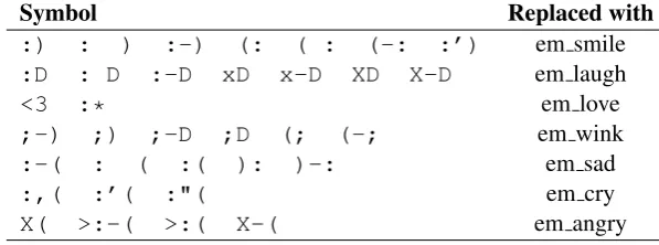
A total of 244 different Emojis were found in the data. From them, 82 were found in CAG data, 68 were found in OAG data and 214 were found in NAG data. Further, the use of emojis was highly overlapped over all the classes, which means that emojis could not serve as a good feature for classification. In day to day social media writing, people often use the symbolic emojis. This step handles such emojies which are not in form of regular emoji. Table 2 shows the replacements done.

Another major consideration was the use of slang/informal abbreviation 45. The slang has a major contribution in classifying the data as stated in (Theodora Chu and Wang, 2016). For example, in many comments, a Hindi informal abbreviation ”bc” word was used. It is similar to Engish informal abbreviation ”fk” which translate to ”fuck”. Having such word are likely to be categorized as OAG. So, such Hindi/English words are pre-processed to the actual meaning (refer Table 1). These pre-processing rules (or sets of regular expressions) were defined as a part of the original work. The rules were written after analysing the dataset and the same could be found in the Appendix A.

4

https://blogs.transparent.com/hindi/slang-in-hindi-i/

Symbol Replaced with :) : ) :-) (: ( : (-: :’) em smile

:D : D :-D xD x-D XD X-D em laugh

<3 :* em love

;-) ;) ;-D ;D (; (-; em wink

:-( : ( :( ): )-: em sad

:,( :’( :"( em cry

X( >:-( >:( X-( em angry

Table 2: Symbolic Emoji Replacement

Normally, when using TFIDF, most repeated words are ranked lower than rare words, but in this corpus, most repeated words like ”BJP”, ”JNU”, ”MODI” were a deciding factor of the class. It is impossible to narrow it down manually on the keywords. Though, old papers (Frank et al., 1999) and (Li et al., 2010) talk about the importance of ”Domain-Specific Keyphrase Extraction” and ”Keyword Extraction for Social Snippets”. It shows that we can build a model that does automatic keyphrase extraction but again it depends upon which type of text are you using. On the other hand Zhang and LeCun (2015) claim that without any knowledge of the syntactic or semantic structure of a language, their model can outperform state of art models. Though, it sounds more convenient to present domain-specific keyphrase extraction to training model.

Lastly, the class distribution over the corpus. The provided data for OAG, CAG, and NAG is, 22.30%, 35.40%, and 42.30% for English and 40%, 41%, and 19% for Hindi, respectively. This can be taken into account if basic assumption of statistical machine learning is considered.

In summarization, data property is one of the important factors which need to be counted for high accuracy of the system.

3.2 Methodology

Nowadays there are many technologies for text classification and one of them is FastText (Joulin et al., 2016a). It provides word vectors for 157 languages and supervised models for 8 datasets using a character level n-gram approach (Joulin et al., 2016b). The next sub-section presents the different text data representation the experiments done with them.

3.2.1 Text Representation

The English data representation was done using Tokenizer6 and GloVe (Pennington et al., 2014) pre-trained word vectors. On another hand, Scikit-Learn API (Buitinck et al., 2013) was used for Tokenizing Hindi data.

A sequential model can be designed for text classification where the text sequence is fed to the machine learning algorithm. Nonetheless, these models only use numerical data and therefore a conversion was needed which involves two subprocesses: Integer Encoding and One-Hot Encoding (Lantz, 2013).

In the Integer Encoding, each unique word/text value is assigned an integer value. For example, ”red” is 1, ”green” is 2, and ”blue” is 3. This process is known as label encoding or an integer encoding and is easily reversible. The idea of one-hot encoding is to replace the integer representation with binary. This means, integer encoded variable is removed and a new binary variable is added for each unique integer value.

3.2.2 Linear Models

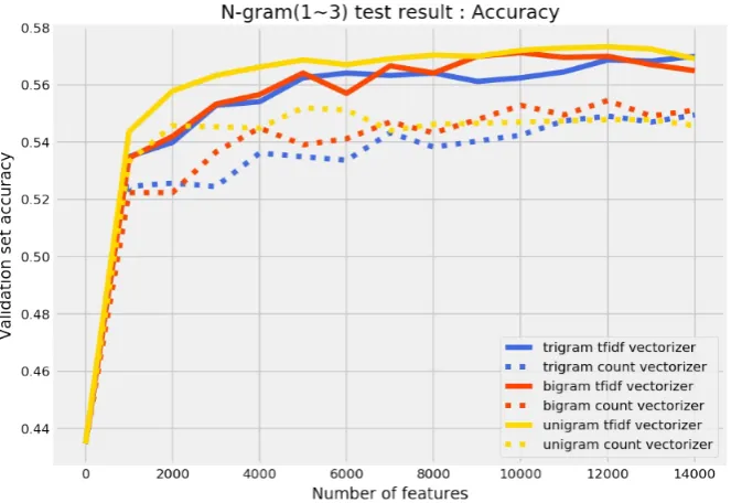
Many research works shows that for small datasets people tend to use linear models. Usually, linear models are fed with different word representations like unigram, bigram, and trigram. Hence, a model using Logistic Regression with n-gram(1-3) was created and the results are shown in Figure 1.

From the figure 1, one can see that TFIDF unigram has the highest test accuracy because the dataset has unique tokens like ”BJP”, ”JNU”, ”MODI”, ”PAK”, etc which are the deciding factor of the class.

Figure 1: Logistic Regression with N-gram(1-3)

So a TFIDF unigram representation along with sklearn machine learning libraries was used to train the model. Table 3 shows the accuracy results with different sklearn linear models like Logistic Regression, SVC, Multinomial NB, Bernoulli NB, Ridge Classifier, and AdaBoost Classifier. (Here, development set is not equal to the test set.)

Linear Model Acc on Validation Split Acc on Development Set

Logistic Regression 57.20 37.45

Linear SVC 54.65 36.61

Linear SVC with L1-based 55.24 36.92

Multinomial NB 56.86 35.41

Bernoulli NB 53.90 36.51

Ridge Classifier 55.36 34.15

AdaBoost Classifier 51.94 33.78

Table 3: Experiment with Sklearn Linear Models: Unigram

3.2.3 Deep Learning Sequential Models

For the research and development, Keras (Chollet and others, 2015) was used as front-end and Tensorflow (Abadi et al., 2016) as back-end.

Method Acc on Dev (%)

Single layer LSTM 37.93

Multi layer LSTM 39.20

Conv1D & GlobalMaxPooling1D 37.37 Conv1D & MaxPooling1D with Hidden Layer 37.73 Convolutional Layers with LSTM 39.03 Convolutional Layers with Bidirectional LSTM 37.53 Fasttext Text Classification 54.00 Fasttext Text Classification with Skip Gram Model 37.00 Fasttext with Conv1D , MaxPooling1D & Bidirectional LSTM 38.53 Multiple Input RNN with Keras 37.00 Concatenate: 2 Bidirectional 38.00 Concatenate: Bidirectional with Conv1D & MaxPooling1D 37.50

Table 4: Results Using Different Deep Learning Algorithms/Layers

3.2.4 Fully Connected Neural Network with Advance Preprocessor & One-Hot Representation

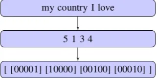
After experimenting with lots of different methods and algorithms, a simple Dense7architecture was used to design the final model for submission. As discussed in Section 3.1, a specific language pre-processor was developed. This pre-processor takes care of exempted stop words, regional level abbreviations, emoji, and text segmentation. Regarding the data representation, a word dictionary was created, in which all the unique words were indexed and the index was used as the word id. These ids were portrayed as a binary matrix with the help of one-hot representation preserving the word orded of the sentences. Consider the figure 2 for better understanding. Assuming the dictionary{”country”: 1, ”very”: 2, ”I”: 3, ”love”: 4, ”my”: 5}.

Figure 2: Word Representation

Here, in the figure 2, both sentences use the same words set but their sentence structure is preserved using dictionary index and one-hot representation.

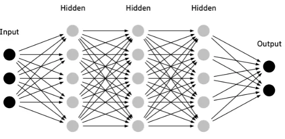
The figure 3 represents the architecture layers of the Dense Neural Network. After several iterations, the number of layers for the architecture was set to three. The 1st hidden layer is having 1024 nodes which take the input from the input layer and the 2nd layer had 512 nodes and the last layer had 256 nodes. Inbetween each layers, mathamatical activation functions like Relu, Sigmoid and Softmax were used. The ordering of this activation function had very high impact on the results. The result of this model is discussed in the section 4.

4 Results and Discussion

Four different test set categories were presented on the shared task: English - Facebook/Twitter and Hindi - Facebook/Twitter

Participants were allowed to submit a maximum of 3 systems for each category and, as such, 3 systems were submitted: Dense, Fasttext and Voting of the two. Tables 5, 6, 7 and 8 show the results, namely the

Figure 3: Dense System Architecture

F1 measure, of the 3 systems for each category. These results were given by the organizing committee.

System F1 (weighted) Random Baseline 0.3535

Dense 0.5813

Fasttext 0.5753 Voting 0.5698

Table 5: English (Facebook) Models.

System F1 (weighted) Random Baseline 0.3477

Dense 0.6009

Fasttext 0.5544 Voting 0.5324

Table 6: English (Twitter) Models.

System F1 (weighted) Random Baseline 0.3571

Dense 0.5951

Fasttext 0.5838 Voting 0.5634

Table 7: Hindi (Facebook) Models.

System F1 (weighted) Random Baseline 0.3206

Dense 0.4830

Fasttext 0.4528 Voting 0.4437

Table 8: Hindi (Twitter) Models.

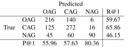
Tables 9, 10, 11 and 12 present confusion matrix with precision and recall for the Dense model (the best model) in each category.

Predicted

OAG CAG NAG R@1 OAG 83 38 23 57.64 True CAG 31 67 44 47.18 NAG 91 190 349 55.40 P@1 40.49 22.71 83.89

Table 9: Confusion matrix of Dense Model -English (Facebook) task.

Predicted

OAG CAG NAG R@1 OAG 230 113 18 63.71 True CAG 143 169 101 40.92 NAG 6 120 357 73.91 P@1 60.69 42.04 75

Table 10: Confusion matrix of Dense Model -English (Twitter) task.

The observation from the tables 5–8 is that the Neural Network model is outperforming Fasttext classification model in all categories. Especially, for Twitter classifier.

Table 9 and 11 shows that for OAG class in Facebook (English/Hindi) dataset, precision is varying between 40.49 to 55.96 and the recall is varying between 57.64 to 59.67 and for CAG class, precision is varying between 22.71 to 57.63 and the recall is varying between 47.18 to 65.86.

Predicted

OAG CAG NAG R@1 OAG 216 140 6 59.67 True CAG 125 272 16 65.86 NAG 45 60 90 46.15 P@1 55.96 57.63 80.36

Table 11: Confusion matrix of Dense Model -Hindi (Facebook) task.

Predicted

OAG CAG NAG R@1 OAG 254 146 59 55.34 True CAG 143 166 72 43.57 NAG 76 123 155 43.79 P@1 53.70 38.16 54.20

Table 12: Confusion matrix of Dense Model -Hindi (Twitter) task.

between 53.70 to 60.69 and the recall is varying between 55.34 to 63.71 and for CAG class, precision is varying between 38.16 to 42.04 and the recall is varying between 40.92 to 43.57.

In the given context of aggression, hate speech, offensive, and abusive language identification, it is important to identify the aggressive or hate speech keywords. This leads to identifying the OAG and CAG classes with higher recall value. At the same time, it is important to identify contexts in which some words may be hateful. Because simply detecting the words will lead to a lot of false positives even if it does raise the recall.

As mentioned, for a demanding task like aggression identification, the proposed model should not have a lower recall for OAG and CAG classes. Further, it could be identified that systems are suffering from false positive values. This could be overcome by reducing class imbalance or oversampling the positive class (OAG & CAG) or changing the weight of examples.

Below is the official ranking of the models among different categories. This ranking was provided by the organizing committee.

English (Facebook) English (Twitter) Hindi (Facebook) Hindi (Twitter) 14thout of 30 1stout of 30 7thout of 15 3rdout of 15

Table 13: Global Standing of Models: vista.ue

5 Conclusion

After discussing different text classification models, one can surely say that Automatic Aggression Identification is necessary and researchers should put more efforts in making it more robust and precise. From all the experiments and models, the designed model with a Dense architecture performs better than a Fasttext model for all four categories. In fact, the system submitted for English - Twitter stood 1st rank for its category. Between the Facebook and Twitter test dataset contents, the model trained over Facebook dataset can be used for unknown Twitter test set but vice-versa is not true. The main reason for this can be a length of sentence, amounts of hashtags, citation of users (i.e ’@’ and the amount of retweet).

In this model words that are not found in the dictionary are omitted. As future work, and to address this issue, a neighboring or similar word could be used; here each word would be added to a list from which neighboring/similar word would be founded. This will help in categorizing unseen words to the model. Thus, all the words are included and there is no omission of words. Another line of future work can be to include semantic meaning from the sentences, extracting ontological features either by Part of Speech (POS) tagging or Entity Extraction (EE).

Acknowledgements

References

Mart´ın Abadi, Paul Barham, Jianmin Chen, Zhifeng Chen, Andy Davis, Jeffrey Dean, Matthieu Devin, Sanjay Ghemawat, Geoffrey Irving, Michael Isard, Manjunath Kudlur, Josh Levenberg, Rajat Monga, Sherry Moore, Derek G. Murray, Benoit Steiner, Paul Tucker, Vijay Vasudevan, Pete Warden, Martin Wicke, Yuan Yu, and

Xiaoqiang Zheng. 2016. Tensorflow: A system for large-scale machine learning. InProceedings of the 12th

USENIX Conference on Operating Systems Design and Implementation, OSDI’16, pages 265–283, Berkeley,

CA, USA. USENIX Association.

Sumeet Agarwal, Shantanu Godbole, Diwakar Punjani, and Shourya Roy. 2007. How much noise is too much: A

study in automatic text classification. Seventh IEEE International Conference on Data Mining (ICDM 2007),

pages 3–12.

Christos Baziotis, Nikos Pelekis, and Christos Doulkeridis. 2017. Datastories at semeval-2017 task 4: Deep lstm

with attention for message-level and topic-based sentiment analysis. InProceedings of the 11th International

Workshop on Semantic Evaluation (SemEval-2017), pages 747–754, Vancouver, Canada, August. Association

for Computational Linguistics.

Lars Buitinck, Gilles Louppe, Mathieu Blondel, Fabian Pedregosa, Andreas Mueller, Olivier Grisel, Vlad Niculae, Peter Prettenhofer, Alexandre Gramfort, Jaques Grobler, Robert Layton, Jake VanderPlas, Arnaud Joly, Brian Holt, and Ga¨el Varoquaux. 2013. API design for machine learning software: experiences from the scikit-learn

project. InECML PKDD Workshop: Languages for Data Mining and Machine Learning, pages 108–122.

Pete Burnap and Matthew L Williams. 2015. Cyber hate speech on twitter: An application of machine

classification and statistical modeling for policy and decision making. Policy & Internet, 7(2):223–242.

Franc¸ois Chollet et al. 2015. Keras.https://keras.io.

Maral Dadvar, Dolf Trieschnigg, Roeland Ordelman, and Franciska de Jong. 2013. Improving cyberbullying

detection with user context. InAdvances in Information Retrieval, pages 693–696. Springer.

Thomas Davidson, Dana Warmsley, Michael Macy, and Ingmar Weber. 2017. Automated Hate Speech Detection

and the Problem of Offensive Language. InProceedings of ICWSM.

Karthik Dinakar, Roi Reichart, and Henry Lieberman. 2011. Modeling the detection of textual cyberbullying. In

The Social Mobile Web, pages 11–17.

Mai ElSherief, Vivek Kulkarni, Dana Nguyen, William Yang Wang, and Elizabeth Belding. 2018. Hate Lingo: A

Target-based Linguistic Analysis of Hate Speech in Social Media. arXiv preprint arXiv:1804.04257.

Darja Fiˇser, Tomaˇz Erjavec, and Nikola Ljubeˇsi´c. 2017. Legal Framework, Dataset and Annotation Schema for

Socially Unacceptable On-line Discourse Practices in Slovene. InProceedings of the Workshop Workshop on

Abusive Language Online (ALW), Vancouver, Canada.

Antigoni-Maria Founta, Constantinos Djouvas, Despoina Chatzakou, Ilias Leontiadis, Jeremy Blackburn, Gianluca Stringhini, Athena Vakali, Michael Sirivianos, and Nicolas Kourtellis. 2018. Large Scale Crowdsourcing and

Characterization of Twitter Abusive Behavior. arXiv preprint arXiv:1802.00393.

Eibe Frank, Gordon W. Paynter, Ian Witten, Carl Gutwin, and Craig Nevill-Manning. 1999. Domain-specific keyphrase extraction. 07.

Bj¨orn Gamb¨ack and Utpal Kumar Sikdar. 2017. Using Convolutional Neural Networks to Classify Hate-speech.

InProceedings of the First Workshop on Abusive Language Online, pages 85–90.

Armand Joulin, Edouard Grave, Piotr Bojanowski, and Tomas Mikolov. 2016a. Bag of tricks for efficient text

classification. arXiv preprint arXiv:1607.01759.

Armand Joulin, Edouard Grave, Piotr Bojanowski, and Tomas Mikolov. 2016b. Bag of tricks for efficient text

classification. CoRR, abs/1607.01759.

Ritesh Kumar, Atul Kr. Ojha, Shervin Malmasi, and Marcos Zampieri. 2018a. Benchmarking Aggression

Identification in Social Media. InProceedings of the First Workshop on Trolling, Aggression and Cyberbulling

(TRAC), Santa Fe, USA.

Ritesh Kumar, Aishwarya N. Reganti, Akshit Bhatia, and Tushar Maheshwari. 2018b. Aggression-annotated

Corpus of Hindi-English Code-mixed Data. InProceedings of the 11th Language Resources and Evaluation

Irene Kwok and Yuzhou Wang. 2013. Locate the hate: Detecting Tweets Against Blacks. InTwenty-Seventh AAAI Conference on Artificial Intelligence.

Brett Lantz. 2013. Machine Learning with R. Packt Publishing.

Zhenhui Li, Ding Zhou, Yun-Fang Juan, and Jiawei Han. 2010. Keyword extraction for social snippets. In

Proceedings of the 19th International Conference on World Wide Web, WWW ’10, pages 1143–1144, New

York, NY, USA. ACM.

Shervin Malmasi and Marcos Zampieri. 2017. Detecting Hate Speech in Social Media. InProceedings of the

International Conference Recent Advances in Natural Language Processing (RANLP), pages 467–472.

Shervin Malmasi and Marcos Zampieri. 2018. Challenges in Discriminating Profanity from Hate Speech.Journal

of Experimental & Theoretical Artificial Intelligence, 30:1–16.

Chikashi Nobata, Joel Tetreault, Achint Thomas, Yashar Mehdad, and Yi Chang. 2016. Abusive Language

Detection in Online User Content. In Proceedings of the 25th International Conference on World Wide Web,

pages 145–153. International World Wide Web Conferences Steering Committee.

Jeffrey Pennington, Richard Socher, and Christopher D. Manning. 2014. Glove: Global vectors for word

representation. InEmpirical Methods in Natural Language Processing (EMNLP), pages 1532–1543.

Anna Schmidt and Michael Wiegand. 2017. A Survey on Hate Speech Detection Using Natural Language

Processing. InProceedings of the Fifth International Workshop on Natural Language Processing for Social

Media. Association for Computational Linguistics, pages 1–10, Valencia, Spain.

Alexandra Schofield and Thomas Davidson. 2017. Identifying Hate Speech in Social Media. XRDS: Crossroads,

The ACM Magazine for Students, 24(2):56–59.

Kylie Jue Theodora Chu and Max Wang. 2016. Comment abuse classification with deep learning.

Zeerak Waseem and Dirk Hovy. 2016. Hateful symbols or hateful people? predictive features for hate speech

detection on twitter. In Proceedings of the NAACL Student Research Workshop, pages 88–93, San Diego,

California, June. Association for Computational Linguistics.

Zeerak Waseem, Thomas Davidson, Dana Warmsley, and Ingmar Weber. 2017. Understanding Abuse: A

Typology of Abusive Language Detection Subtasks. InProceedings of the First Workshop on Abusive Langauge

Online.

Xiang Zhang and Yann LeCun. 2015. Text understanding from scratch.CoRR, abs/1502.01710.

Ziqi Zhang, David Robinson, and Jonathan Tepper. 2018. Detecting Hate Speech on Twitter Using a

Appendix A Regional Level Abbreviations

FLAGS = r e . MULTILINE | r e . DOTALL

d e f t o k e n i z e ( t e x t ) :

# D i f f e r e n t r e g e x p a r t s f o r s m i l e y f a c e s e y e s = r ” [ 8 : = ; ] ”

n o s e = r ” [ ’ ‘\ −] ? ”

# f u n c t i o n

d e f r e s u b ( p a t t e r n , r e p l ) :

r e t u r n r e . s u b ( p a t t e r n , r e p l , t e x t , f l a g s =FLAGS )

t e x t = r e s u b ( r ” h t t p s ? :\/\/\S+\b|www\. (\w+\. ) +\S∗” , ” u r l ” ) # S m i l e −− : ) , : ) , :−) , ( : , ( : , (−: , : ’ )

t e x t = r e s u b ( r ” ( :\s ?\)|:− \)| \(\s ? :| \( −:|:\ ’\) ) ” , ” e m s m i l e ” ) # Laugh −− : D , : D , :−D , xD , x−D , XD, X−D

t e x t = r e s u b ( r ” ( :\s ?D|:−D|x−?D|X−?D ) ” , ” e m l a u g h ” ) # Love −− <3 , :∗

t e x t = r e s u b ( r ” (<3|:\ ∗) ” , ” e m l o v e ” ) # Wink −− ;−) , ; ) , ;−D , ; D , ( ; , (−;

t e x t = r e s u b ( r ” ( ;−?\)|;−?D| \( −? ; ) ” , ” em wink ” ) # Sad −− :−( , : ( , : ( , ) : , )−:

t e x t = r e s u b ( r ’ ( :\s ?\(|:− \(| \)\s ? :| \)−: ) ’ , ” e m s a d ” ) # Cry −− : , ( , : ’ ( , : ” (

t e x t = r e s u b ( r ’ ( : ,\(|:\ ’\(|: ”\( ) ’ , ” e m c r y ” ) # remove f u n n n n n y −−> f u n n y

t e x t = r e s u b ( r ” ( . )\1 + ” , r ”\1\1 ” ) # remove &

t e x t = r e s u b ( r ” (− | \’ ) ” , ” ” )

t e x t = r e s u b ( r ”@[0−9]+−” , ” number ” ) t e x t = r e s u b ( r ”{ } { }[ ) dD ] +|[ ) dD ] +{ } { }” .

f o r m a t ( e y e s , n o s e , n o s e , e y e s ) , ” e m p o s i t i v e ” )

t e x t = r e s u b ( r ”{}{}p + ” . f o r m a t ( e y e s , n o s e ) , ” e m p o s i t i v e ” ) t e x t = r e s u b ( r ”{ } { } \( +| \) +{ } { }” .

f o r m a t ( e y e s , n o s e , n o s e , e y e s ) , ” e m n e g a t i v e ” ) t e x t = r e s u b ( r ”{ } { }[\/|l∗] ” .

f o r m a t ( e y e s , n o s e ) , ” e m n e u t r a l f a c e ” ) t e x t = r e s u b ( r ’−’ , r ’ ’ )

t e x t = r e s u b ( r ” ( [ p l s ? s ] ){2 ,}” , r ”\1 ” ) t e x t = r e s u b ( r ” ( [ p l z ? z ] ){2 ,}” , r ”\1 ” ) t e x t = r e s u b ( r ’\ \n ’ , r ’ ’ )

t e x t = r e s u b ( r ” s x ” , ” s e x ” ) t e x t = r e s u b ( r ” u ” , ” you ” ) t e x t = r e s u b ( r ” r ” , ” a r e ” ) t e x t = r e s u b ( r ” y ” , ” why ” ) t e x t = r e s u b ( r ” Y ” , ” WHY ” ) t e x t = r e s u b ( r ”Y ” , ” WHY ” ) t e x t = r e s u b ( r ” hv ” , ” h a v e ” ) t e x t = r e s u b ( r ” c ” , ” s e e ” )

t e x t = r e s u b ( r ” c o z ” , ” b e c a u s e ” ) t e x t = r e s u b ( r ” v ” , ” we ” )

t e x t = r e s u b ( r ” p p l ” , ” p e o p l e ” ) t e x t = r e s u b ( r ” p e p l ” , ” p e o p l e ” ) t e x t = r e s u b ( r ” r b i ” , ” r b i ” ) t e x t = r e s u b ( r ” R B I ” , ” RBI ” ) t e x t = r e s u b ( r ” R b i ” , ” r b i ” ) t e x t = r e s u b ( r ” R ” , ” ARE ” ) t e x t = r e s u b ( r ” hav ” , ” h a v e ” ) t e x t = r e s u b ( r ”R ” , ” ARE ” ) t e x t = r e s u b ( r ” U ” , ” you ” ) t e x t = r e s u b ( r ”U ” , ” you ” )

t e x t = r e s u b ( r ” p l s ” , ” p l e a s e ” ) t e x t = r e s u b ( r ” P l s ” , ” P l e a s e ” ) t e x t = r e s u b ( r ” p l z ” , ” p l e a s e ” ) t e x t = r e s u b ( r ” P l z ” , ” P l e a s e ” ) t e x t = r e s u b ( r ”PLZ ” , ” P l e a s e ” ) t e x t = r e s u b ( r ” P l s ” , ” P l e a s e ” ) t e x t = r e s u b ( r ” p l z ” , ” p l e a s e ” ) t e x t = r e s u b ( r ” P l z ” , ” P l e a s e ” ) t e x t = r e s u b ( r ”PLZ ” , ” P l e a s e ” )

t e x t = r e s u b ( r ” t h a n k z ” , ” t h a n k s ” ) t e x t = r e s u b ( r ” t h n x ” , ” t h a n k s ” ) t e x t = r e s u b ( r ” f u c k\w+ ” , ” f u c k ” ) t e x t = r e s u b ( r ” f\∗\∗ ” , ” f u c k ” ) t e x t = r e s u b ( r ”\ ∗\ ∗\ ∗k ” , ” f u c k ” ) t e x t = r e s u b ( r ” F\∗\∗ ” , ” f u c k ” )

t e x t = r e s u b ( r ”mo\∗\∗\∗\∗\∗ ” , ” f u c k e r ” ) t e x t = r e s u b ( r ” b\∗\∗\∗\∗ ” , ” b l o d y ” ) t e x t = r e s u b ( r ” mc ” , ” f u c k e r ” ) t e x t = r e s u b ( r ” MC ” , ” f u c k e r ” ) t e x t = r e s u b ( r ” w t f ” , ” f u c k ” )

t e x t = r e s u b ( r ” ch\∗\∗\∗ya ” , ” f u c k e r ” ) t e x t = r e s u b ( r ” ch\∗\∗Tya ” , ” f u c k e r ” ) t e x t = r e s u b ( r ” ch\∗\∗T i a ” , ” f u c k e r ” ) t e x t = r e s u b ( r ” C\∗\∗\∗y a s ” , ” f u c k e r ” ) t e x t = r e s u b ( r ” l\∗\∗\∗\∗ ” , ” s h i t ” )

t e x t = r e s u b ( r ” A\∗\∗\∗\∗\∗\∗S ” , ” ASSHOLES ” ) t e x t = r e s u b ( r ” d i\∗\∗\∗\∗s ” , ” f u c k e r ” ) t e x t = r e s u b ( r ” nd ” , ” and ” )

t e x t = r e s u b ( r ”Nd ” , ” and ” )

t e x t = r e s u b ( r ” ( i n d [ v s ] pak ) ” , ” i n d i a v e r s u s p a k i s t a n ” ) t e x t = r e s u b ( r ” ( pak [ v s ] i n d ) ” , ” p a k i s t a n v e r s u s i n d i a ” ) t e x t = r e s u b ( r ” ( i n d v s u a e ) ” ,

” i n d i a v e r s u s U n i t e d Arab E m i r a t e s ” )

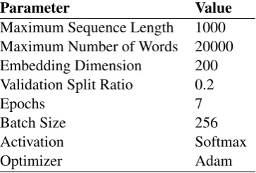
Appendix B Deep Learning Sequential Models

Parameter Value

Maximum Sequence Length 1000 Maximum Number of Words 20000 Embedding Dimension 200 Validation Split Ratio 0.2

Epochs 7

Batch Size 256

Activation Softmax

Optimizer Adam