Shared Logistic Normal Distributions for Soft Parameter Tying in Unsupervised Grammar Induction

Shared Logistic Normal Distributions for Soft Parameter Tying

in Unsupervised Grammar Induction

Shay B. Cohen and Noah A. Smith Language Technologies Institute

School of Computer Science Carnegie Mellon University Pittsburgh, PA 15213, USA {scohen,nasmith_}@cs.cmu.edu

Abstract

We present a family of priors over probabilis-tic grammar weights, called the shared logisprobabilis-tic normal distribution. This family extends the partitioned logistic normal distribution, en-abling factored covariance between the prob-abilities of different derivation events in the probabilistic grammar, providing a new way to encode prior knowledge about an unknown grammar. We describe a variational EM al-gorithm for learning a probabilistic grammar based on this family of priors. We then experi-ment with unsupervised dependency grammar induction and show significant improvements using our model for both monolingual learn-ing andbilinguallearning with a non-parallel, multilingual corpus.

1 Introduction

Probabilistic grammars have become an important tool in natural language processing. They are most commonly used for parsing and linguistic analy-sis (Charniak and Johnson, 2005; Collins, 2003), but are now commonly seen in applications like ma-chine translation (Wu, 1997) and question answer-ing (Wang et al., 2007). An attractive property of probabilistic grammars is that they permit the use of well-understood parameter estimation methods forlearning—both from labeled and unlabeled data. Here we tackle the unsupervised grammar learning problem, specifically for unlexicalized context-free dependency grammars, using an empirical Bayesian approach with a novel family of priors.

There has been an increased interest recently in employing Bayesian modeling for probabilistic grammars in different settings, ranging from putting priors over grammar probabilities (Johnson et al.,

2007) to putting non-parametric priors over deriva-tions (Johnson et al., 2006) to learning the set of states in a grammar (Finkel et al., 2007; Liang et al., 2007). Bayesian methods offer an elegant frame-work for combining prior knowledge with data. The main challenge in Bayesian grammar learning is efficiently approximating probabilistic inference, which is generally intractable. Most commonly vari-ational (Johnson, 2007; Kurihara and Sato, 2006) or sampling techniques are applied (Johnson et al., 2006).

Because probabilistic grammars are built out of multinomial distributions, the Dirichlet family (or, more precisely, a collection of Dirichlets) is a natural candidate for probabilistic grammars because of its conjugacy to the multinomial family. Conjugacy im-plies a clean form for the posterior distribution over grammar probabilities (given the data and the prior), bestowing computational tractability.

Following work by Blei and Lafferty (2006) for topic models, Cohen et al. (2008) proposed an alter-native to Dirichlet priors for probabilistic grammars, based on the logistic normal (LN) distribution over the probability simplex. Cohen et al. used this prior to softly tie grammar weights through the covariance parameters of the LN. The prior encodes informa-tion about which grammar rules’ weights are likely to covary, a more intuitive and expressive represen-tation of knowledge than offered by Dirichlet distri-butions.1

The contribution of this paper is two-fold. First, from the modeling perspective, we present a gen-eralization of the LN prior of Cohen et al. (2008), showing how to extend the use of the LN prior to

1_{Although the task, underlying model, and weights being}

tied were different, Eisner (2002) also showed evidence for the efficacy of parameter tying in grammar learning.

tie betweenanygrammar weights in a probabilistic grammar (instead of only allowing weights within the same multinomial distribution to covary). Sec-ond, from the experimental perspective, we show how such flexibility in parameter tying can help in unsupervised grammar learning in the well-known monolingual setting and in a new bilingual setting where grammars for two languages are learned at once (without parallel corpora).

Our method is based on a distribution which we call theshared logistic normal distribution, which is a distribution over a collection of multinomials from different probability simplexes. We provide a variational EM algorithm for inference.

The rest of this paper is organized as follows. In

§2, we give a brief explanation of probabilistic gram-mars and introduce some notation for the specific type of dependency grammar used in this paper, due to Klein and Manning (2004). In§3, we present our model and a variational inference algorithm for it. In

§4, we report on experiments for both monolingual

settings and a bilingual setting and discuss them. We discuss future work (§5) and conclude in§6.

2 Probabilistic Grammars and Dependency Grammar Induction

A probabilistic grammar defines a probability dis-tribution over grammatical derivations generated through a step-by-step process. HMMs, for exam-ple, can be understood as a random walk through a probabilistic finite-state network, with an output symbol sampled at each state. Each “step” of the walk and each symbol emission corresponds to one derivation step. PCFGs generate phrase-structure trees by recursively rewriting nonterminal symbols as sequences of “child” symbols (each itself either a nonterminal symbol or a terminal symbol analo-gous to the emissions of an HMM). Each step or emission of an HMM and each rewriting operation of a PCFG is conditionally independent of the other rewriting operations given a single structural ele-ment (one HMM or PCFG state); this Markov prop-erty permits efficient inference for the probability distribution defined by the probabilistic grammar.

In general, a probabilistic grammar defines the joint probability of a string x and a grammatical

derivationy:

p(x,y_|θ) = K

Y

k=1

Nk

Y

i=1

θfk,i(x,y)

k,i (1)

= exp

K

X

k=1

Nk

X

i=1

fk,i(x,y) logθk,i

where fk,i is a function that “counts” the number of times the kth distribution’s ith event occurs in the derivation. The θ are a collection of K multi-nomialshθ1, ...,θKi, thekth of which includesNk events. Note that there may be many derivationsy

for a given stringx—perhaps even infinitely many in some kinds of grammars.

2.1 Dependency Model with Valence

HMMs and PCFGs are the best-known probabilis-tic grammars, but there are many others. In this paper, we use the “dependency model with va-lence” (DMV), due to Klein and Manning (2004). DMV defines a probabilistic grammar for unla-beled, projective dependency structures. Klein and Manning (2004) achieved their best results with a combination of DMV with a model known as the “constituent-context model” (CCM). We do not ex-periment with CCM in this paper, because it does not fit directly in a Bayesian setting (it is highly defi-cient) and because state-of-the-art unsupervised de-pendency parsing results have been achieved with DMV alone (Smith, 2006).

Using the notation above, DMV defines x =

hx1, x2, ..., xni to be a sentence. x0 is a special

“wall” symbol, $, on the left of every sentence. A tree y is defined by a pair of functions yleft and

yright (both{0,1,2, ..., n} → 2{1,2,...,n}_{) that map} each word to its sets of left and right dependents, respectively. Here, the graph is constrained to be a projectivetree rooted atx0= $: each word except $

has a single parent, and there are no cycles or cross-ing dependencies. yleft(0)is taken to be empty, and

yright(0) contains the sentence’s single head. Let

y(i) _{denote the subtree rooted at position i. The}

probability P(y(i) _| xi,θ) of generating this sub-tree, given its head wordxi, is defined recursively, as described in Fig. 1 (Eq. 2).

The probability of the entire tree is given by p(x,y _|θ) = P(y(0) _{|$,θ). Theθare the}

P(y(i) _|xi,θ) = Q_{D∈{left,right}}θs(stop|xi,D,[yD(i) =∅]) (2)

×Qj∈yD(i)θs(¬stop|xi,D,firsty(j))×θc(xj |xi,D)×P(y (j)_|x

j,θ)

Figure 1: The “dependency model with valence” recursive equation.firsty(j)is a predicate defined to be true iffxjis

the closest child (on either side) to its parentxi. The probability of the treep(x,y|θ) =P(y(0)|$,θ).

follow the general setting of Eq. 1, we index these distributions asθ1, ...,θK.

Headden et al. (2009) extended DMV so that the distributions θc condition on the valence as well, with smoothing, and showed significant improve-ments for short sentences. Our experiimprove-ments found that these improvements do not hold on longer sen-tences. Here we experiment only with DMV, but note that our techniques are also applicable to richer probabilistic grammars like that of Headden et al.

2.2 Learning DMV

Klein and Manning (2004) learned the DMV prob-abilities θ from a corpus of part-of-speech-tagged sentences using the EM algorithm. EM manipulates θto locally optimize the likelihood of the observed portion of the data (here, x), marginalizing out the hidden portions (here, y). The likelihood surface is not globally concave, so EM only locally opti-mizes the surface. Klein and Manning’s initializa-tion, though reasonable and language-independent, was an important factor in performance.

Various alternatives to EM were explored by Smith (2006), achieving substantially more accu-rate parsing models by altering the objective func-tion. Smith’s methods did require substantial hyper-parameter tuning, and the best results were obtained using small annotated development sets to choose hyperparameters. In this paper, we consider only fully unsupervised methods, though we the Bayesian ideas explored here might be merged with the bias-ing approaches of Smith (2006) for further benefit.

3 Parameter Tying in the Bayesian Setting As stated above,θ comprises a collection of multi-nomials that weights the grammar. Taking the Bayesian approach, we wish to place a prior on those multinomials, and the Dirichlet family is a natural candidate for such a prior because of its conjugacy,

which makes inference algorithms easier to derive. For example, if we make a “mean-field assumption,” with respect to hidden structure and weights, the variational algorithm for approximately inferring the distribution overθ and treesy resembles the tradi-tional EM algorithm very closely (Johnson, 2007). In fact, variational inference in this case takes an ac-tion similar to smoothing the counts using the exp-Ψ

function during the E-step. Variational inference can be embedded in an empirical Bayes setting, in which we optimize the variational bound with respect to the hyperparameters as well, repeating the process until convergence.

3.1 Logistic Normal Distributions

While Dirichlet priors over grammar probabilities make learning algorithms easy, they are limiting. In particular, as noted by Blei and Lafferty (2006), there is no explicit flexible way for the Dirichlet’s parameters to encode beliefs about covariance be-tween the probabilities of two events. To illustrate this point, we describe how a multinomialθ of di-mensiondis generated from a Dirichlet distribution with parametersα=_hα1, ..., αdi:

1. Generate ηj ∼ Γ(αj,1) independently forj ∈

{1, ..., d_}. 2. θj ←ηj/Piηi.

whereΓ(α,1)is a Gamma distribution with shapeα and scale 1.

Correlation among θi and θj, i 6= j, cannot be modeled directly, only through the normalization in step 2. In contrast, LN distributions (Aitchison, 1986) provide a natural way to model such correla-tion. The LN draws a multinomialθas follows:

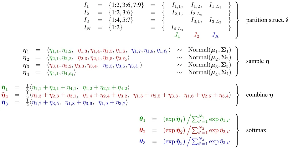
I1 = {1:2,3:6,7:9} = { I1,1, I1,2, I1,L1 } I2 = {1:2,3:6} = { I2,1, I2,L2 } I3 = {1:4,5:7} = { I3,1, I3,L3 }

IN = {1:2} = { I4,L4 }

J1 J2 JK

          

partition struct.S

η1 = hη1,1,η1,2, η1,3,η1,4,η1,5,η1,6, η1,7,η1,8,η1,`1i ∼ Normal(µ1,Σ1) η2 = hη2,1,η2,2, η2,3,η2,4,η2,5,η2,`2i ∼ Normal(µ2,Σ2) η3 = hη3,1,η3,2,η3,3,η3,4, η3,5,η3,6,η3,`3i ∼ Normal(µ3,Σ3)

η4 = hη4,1,η4,`4i ∼ Normal(µ4,Σ4)

      

sampleη

˜

η1 = 13hη1,1+η2,1+η4,1, η1,2+η2,2+η4,2i

˜

η2 = 13hη1,3+η2,3+η3,1, η1,4+η2,4+η3,2, η1,5+η2,5+η3,3, η1,6+η2,6+η3,4i

˜

η3 = 12hη1,7+η3,5, η1,8+η3,6, η1,9+η3,7i

 

 combineη

θ1 = (exp ˜η1)

.PN1

i0=1exp ˜η1,i0

θ2 = (exp ˜η2) .PN2

i0=1exp ˜η2,i0 θ3 = (exp ˜η3)

.PN3

i0=1exp ˜η3,i0

        

softmax

Figure 2: An example of a shared logistic normal distribution, illustrating Def. 1. N = 4experts are used to sample K = 3multinomials;L1 = 3,L2 = 2,L3 = 2,L4 = 1,`1 = 9,`2 = 6,`3 = 7,`4 = 2,N1 = 2,N2 = 4, and

N3= 3. This figure is best viewed in color.

Blei and Lafferty (2006) defined correlated topic models by replacing the Dirichlet in latent Dirich-let allocation models (Blei et al., 2003) with a LN distribution. Cohen et al. (2008) compared Dirichlet and LN distributions for learning DMV using em-pirical Bayes, finding substantial improvements for English using the latter.

In that work, we obtained improvements even without specifying exactly which grammar proba-bilities covaried. While empirical Bayes learning permits these covariances to be discovered without supervision, we found that by initializing the covari-ance to encode beliefs about which grammar prob-abilities should covary, further improvements were possible. Specifically, we grouped the Penn Tree-bank part-of-speech tags into coarse groups based on the treebank annotation guidelines and biased the initial covariance matrix for each child distri-bution θc(_{· | ·},_·) so that the probabilities of child tags from the same coarse group covaried. For ex-ample, the probability that a past-tense verb (VBD) has a singular noun (NN) as a right child may be correlated with the probability that it has a plu-ral noun (NNS) as a right child. Hence linguistic

knowledge—specifically, a coarse grouping of word classes—can be encoded in the prior.

A per-distribution LN distribution only permits probabilities within a multinomial to covary. We will generalize the LN to permit covariance among any probabilities in θ, throughout the model. For example, the probability of a past-tense verb (VBD) having a noun as a right child might correlate with the probability that other kinds of verbs (VBZ, VBN, etc.) have a noun as a right child.

3.2 Shared Logistic Normal Distributions To solve this problem, we suggest a refinement of the class of PLN distributions. Instead of using a single normal vector for all of the multinomials, we use several normal vectors, partition each one and thenrecombineparts which correspond to the same multinomial, as a mixture. Next, we apply the lo-gisitic transformation on the mixed vectors (each of which is normally distributed as well). Fig. 2 gives an example of a non-trivial case of using a SLN distribution, where three multinomials are generated from four normal experts.

We now formalize this notion. For a natural num-berN, we denote by1:N the set _{1, ..., N_}. For a vector in v ∈ RN _{and a set I ⊆ 1:N, we denote} by vI to be the vector created from v by using the coordinates in I. Recall that K is the number of multinomials in the probabilistic grammar, andNk is the number of events in thekth multinomial. Definition 1. We define a shared logistic nor-mal distribution with N “experts” over a collec-tion of K multinomial distributions. Let η_{n ∼}

Normal(µ_n,Σn) be a set of multivariate normal variables for n _∈ 1:N, where the length of η_n is denoted `n. Let In = {In,j}L<sub>j=1</sub>n be a parti-tion of 1:`n into Ln sets, such that ∪L_j=1n In,j =

1:`n and In,j ∩ In,j0 = ∅ for j 6= j0. Let J<sub>k</sub> for k <sub>∈</sub> 1:K be a collection of (disjoint) sub-sets of {In,j | n ∈ 1:N, j ∈ 1:`n,|In,j| = Nk}, such that all sets in Jk are of the same size, Nk. Let η˜k = _|J1k|

P

In,j∈Jkηn,In,j, and θk,i =

exp(˜ηk,i)Pi0exp(˜ηk,i0). We then sayθdistributes according to theshared logistic normal distribution with partition structure S = (_{In}Nn=1,{Jk}Kk=1)

andnormal experts{(µ_n,Σn)}Nn=1and denote it by

θ∼SLN(µ,Σ,S).

The partitioned LN distribution in Aitchison (1986) can be formulated as a shared LN distribution whereN = 1. The LN collection used by Cohen et al. (2008) is the special case where N = K, each Ln= 1, each`k=Nk, and eachJk={Ik,1}.

The covariance among arbitraryθk,iis not defined directly; it is implied by the definition of the nor-mal experts η_n,In,j, for each In,j ∈ Jk. We note that a SLN can be represented as a PLN by relying on the distributivity of the covariance operator, and merging all the partition structure into one (perhaps

sparse) covariance matrix. However, if we are inter-ested in keeping a factored structure on the covari-ance matrices which generate the grammar weights, we cannot represent every SLN as a PLN.

It is convenient to think of each ηi,j as a weight associated with a unique event’s probability, a cer-tain outcome of a cercer-tain multinomial in the prob-abilistic grammar. By letting different ηi,j covary with each other, we loosen the relationships among θk,j and permit the model—at least in principle— to learn patterns from the data. Def. 1 also implies that we multiply several multinomials together in a product-of-experts style (Hinton, 1999), because the exponential of a mixture of normals becomes a prod-uct of (unnormalized) probabilities.

Our extension to the model in Cohen et al. (2008) follows naturally after we have defined the shared LN distribution. The generative story for this model is as follows:

1. Generateθ _∼SLN(µ,Σ,S), whereθis a col-lection of vectorsθk,k= 1, ..., K.

2. Generatexandyfromp(x,y|θ)(i.e., sample from the probabilistic grammar).

3.3 Inference

In this work, the partition structureSisknown, the

sentencesxareobserved, the treesyand the gram-mar weightsθarehidden, and the parameters of the shared LN distributionµandΣarelearned.2

Our inference algorithm aims to find the poste-rior over the grammar probabilitiesθand the hidden structures (grammar trees y). To do that, we use variational approximation techniques (Jordan et al., 1999), which treat the problem of finding the pos-terior as an optimization problem aimed to find the best approximationq(θ,y)of the posteriorp(θ,y_|

x,µ,Σ,S). The posteriorqneeds to be constrained to be within a family of tractable and manageable distributions, yet rich enough to represent good ap-proximations of the true posterior. “Best approx-imation” is defined as the KL divergence between q(θ,y)andp(θ,y_|x,µ,Σ,S).

Our variational inference algorithm uses a mean-field assumption: q(θ,y) = q(θ)q(y). The distri-butionq(θ)is assumed to be a LN distribution with

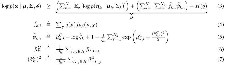
logp(x_|µ,Σ,S) _≥ PN_n=1Eq[logp(ηk|µk,Σk)]

+PK

k=1 PNk

i=1f˜k,iψ˜k,i

+H(q)

| {z }

B

(3)

˜

fk,i , Pyq(y)fk,i(x,y) (4)

˜

ψk,i , µ˜Ck,i−log ˜ζk+ 1−_ζ˜1_k PNk

i0=1exp

˜

µC_k,i+ (˜σ C k,i)2

2

(5)

˜

µC_k , _|J1_k|P_Ir,j∈J

kµ˜r,Ir,j (6)

(˜σC_k)2 , _|J1_k|2

P

Ir,j∈Jkσ˜

2

r,Ir,j (7)

Figure 3: Variational inference bound. Eq. 3 is the bound itself, using notation defined in Eqs. 4–7 for clarity. Eq. 4 defines expected counts of the grammar events under the variational distributionq(y), calculated using dynamic pro-gramming. Eq. 5 describes the weights for the weighted grammar defined byq(y). Eq. 6 and Eq. 7 describe the mean

and the variance, respectively, for the multivariate normal eventually used with the weighted grammar. These values are based on the parameterization ofq(θ)byµ˜i,jand˜σi,j2 . An additional set of variational parameters isζ˜k, which

helps resolve the non-conjugacy of the LN distribution through a first order Taylor approximation.

all off-diagonal covariances fixed at zero (i.e., the variational parameters consist of a single meanµ˜k,i and a single variance σ˜2_k,i for each θk,i). There is an additional variational parameter,ζ˜kper multino-mial, which is the result of an additional variational approximation because of the lack of conjugacy of the LN distribution to the multinomial distribution. The distributionq(y)is assumed to be defined by a DMV with unnormalized probabilitiesψ˜.

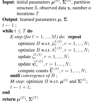
Inference optimizes the bound B given in Fig. 3 (Eq. 3) with respect to the variational parameters. Our variational inference algorithm is derived simi-larly to that of Cohen et al. (2008). Because we wish tolearnthe values ofµandΣ, we embed variational inference as the E step within a variational EM algo-rithm, shown schematically in Fig. 4. In our exper-iments, we use this variational EM algorithm on a training set, and then use the normal experts’ means to get a point estimate forθ, the grammar weights. This is calledempirical Bayesian estimation. Our approach differs from maximuma posteriori(MAP) estimation, since we re-estimate the parameters of the normal experts. Exact MAP estimation is prob-ably not feasible; a variational algorithm like ours might be applied, though better performance is ex-pected from adjusting the SLN to fit the data.

4 Experiments

Our experiments involve data from two treebanks: the Wall Street Journal Penn treebank (Marcus et

al., 1993) and the Chinese treebank (Xue et al., 2004). In both cases, following standard practice, sentences were stripped of words and punctuation, leaving part-of-speech tags for the unsupervised in-duction of dependency structure. For English, we train on§2–21, tune on§22 (without using annotated data), and report final results on§23. For Chinese,

we train on§1–270, use§301–1151 for development

and report testing results on§271–300.3

To evaluate performance, we report the fraction of words whose predicted parent matches the gold standard corpus. This performance measure is also known as attachment accuracy. We considered two parsing methods after extracting a point estimate for the grammar: the most probable “Viterbi” parse (argmaxyp(y|x,θ)) and the minimum Bayes risk

(MBR) parse (argmin_yEp(y0_|x,θ)[`(y;x,y0)]) with

dependency attachment error as the loss function (Goodman, 1996). Performance with MBR parsing is consistently higher than its Viterbi counterpart, so we report only performance with MBR parsing.

4.1 Nouns, Verbs, and Adjectives

In this paper, we use a few simple heuristics to de-cide which partition structureSto use. Our

heuris-3_{Unsupervised training for these datasets can be costly,}

Input: initial parametersµ(0)_,Σ(0)_{, partition} structureS, observed datax, number of

iterationsT

Output: learned parametersµ,Σ t_←1;

whilet_≤T do

E-step (for`= 1, ..., M) do: repeat

optimizeBw.r.t.µ˜`,r(t), r= 1, ..., N;

optimizeBw.r.t.σ˜`,r(t), r= 1, ..., N;

updateζ˜r`,(t), r= 1, ..., N;

updateψ˜`,r(t), r= 1, ..., N;

compute counts˜f`,(t)

r , r= 1, ..., N;

untilconvergence ofB;

M-step: optimizeBw.r.t.µ(t)_andΣ(t)_;

t←t+ 1;

end

returnµ(T)_,Σ(T)

Figure 4: Main details of the variational inference EM algorithm with empirical Bayes estimation ofµandΣ.

Bis the bound defined in Fig. 3 (Eq. 3).Nis the number

of normal experts for the SLN distribution defining the prior. M is the number of training examples. The full

algorithm is given in Cohen and Smith (2009).

tics rely mainly on the centrality of content words: nouns, verbs, and adjectives. For example, in the En-glish treebank, the most common attachment errors (with the LN prior from Cohen et al., 2008) happen with a noun (25.9%) or a verb (16.9%) parent. In the Chinese treebank, the most common attachment errors happen with noun (36.0%) and verb (21.2%) parents as well. The errors being governed by such attachments are the direct result of nouns and verbs being the most common parents in these data sets.

Following this observation, we compare four dif-ferent settings in our experiments (all SLN settings include one normal expert for each multinomial on its own, equivalent to the regular LN setting from Cohen et al.):

• TIEV: We add normal experts that tie all proba-bilities corresponding to a verbal parent (any par-ent, using the coarse tags of Cohen et al., 2008). LetV be the set of part-of-speech tags which be-long to the verb category. For each directionD (left or right), the set of multinomials of the form θc(_{· |}v,D), forv_∈V, all share a normal expert. For each direction Dand each boolean value B

of the predicate firsty(·), the set of multinomials

θs(_{· |}x,D, v), forv _∈V share a normal expert.

• TIEN: This is the same as TIEV, only for nominal parents.

• TIEV&N: Tie both verbs and nouns (in separate

partitions). This is equivalent to taking the union of the partition structures of the above two set-tings.

• TIEA: This is the same as TIEV, only for adjecti-val parents.

Since inference for a model with parameter tying can be computationally intensive, we first run the in-ference algorithm without parameter tying, and then add parameter tying to the rest of the inference algo-rithm’s execution until convergence.

Initialization is important for the inference al-gorithm, because the variational bound is a non-concave function. For the expected values of the normal experts, we use the initializer from Klein and Manning (2004). For the covariance matrices, we follow the setting in Cohen et al. (2008) in our ex-periments also described in§3.1. For each treebank, we divide the tags into twelve disjoint tag families.4 The covariance matrices for all dependency distri-butions were initialized with1on the diagonal,0.5 between tags which belong to the same family, and

0 otherwise. This initializer has been shown to be more successful than an identity covariance matrix.

4.2 Monolingual Experiments

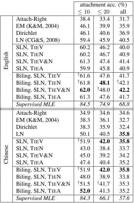
We begin our experiments with a monolingual set-ting, where we learn grammars for English and Chi-nese (separately) using the settings described above. The attachment accuracy for this set of experi-ments is described in Table 1. The baselines include right attachment (where each word is attached to the word to its right), MLE via EM (Klein and Man-ning, 2004), and empirical Bayes with Dirichlet and LN priors (Cohen et al., 2008). We also include a “ceiling” (DMV trained using supervised MLE from the training sentences’ trees). For English, we see that tying nouns, verbs or adjectives improves per-formance compared to the LN baseline. Tying both nouns and verbs improves performance a bit more.

4_{These are simply coarser tags: adjective, adverb,}

attachment acc. (%)

≤10 ≤20 all

English

Attach-Right 38.4 33.4 31.7

EM (K&M, 2004) 46.1 39.9 35.9

Dirichlet 46.1 40.6 36.9

LN (CG&S, 2008) 59.4 45.9 40.5

SLN, TIEV 60.2 46.2 40.0

SLN, TIEN 60.2 46.7 40.9

SLN, TIEV&N 61.3 47.4 41.4

SLN, TIEA 59.9 45.8 40.9

Biling. SLN, TIEV †61.6 47.6 41.7

Biling. SLN, TIEN †61.8 48.1 †42.1

Biling. SLN, TIEV&N 62.0 †48.0 42.2

Biling. SLN, TIEA 61.3 47.6 41.7 Supervised MLE 84.5 74.9 68.8

Chinese

Attach-Right 34.9 34.6 34.6

EM (K&M, 2004) 38.3 36.1 32.7

Dirichlet 38.3 35.9 32.4

LN 50.1 40.5 35.8

SLN, TIEV †51.9 42.0 35.8

SLN, TIEN 43.0 38.4 33.7

SLN, TIEV&N 45.0 39.2 34.2

SLN, TIEA 47.4 40.4 35.2

Biling. SLN, TIEV †_{51.9 42.0 35.8} Biling. SLN, TIEN 48.0 38.9 33.8 Biling. SLN, TIEV&N †_51.5 †_{41.7 35.3} Biling. SLN, TIEA 52.0 41.3 35.2

Supervised MLE 84.3 66.1 57.6

Table 1: Attachment accuracy of different models, on test data from the Penn Treebank and the Chinese Treebank of varying levels of difficulty imposed through a length filter. Attach-Right attaches each word to the word on its right and the last word to $. Bold marks best overall accuracy per length bound, and_†marks figures that are not significantly worse (binomial sign test,p <0.05).

4.3 Bilingual Experiments

Leveraging information from one language for the task of disambiguating another language has re-ceived considerable attention (Dagan, 1991; Smith and Smith, 2004; Snyder and Barzilay, 2008; Bur-kett and Klein, 2008). Usually such a setting re-quires a parallel corpus or other annotated data that ties between those two languages.5

Our bilingual experiments use the English and Chinese treebanks, which are not parallel corpora, to train parsers for both languages jointly.

Shar-5_{Haghighi et al. (2008) presented a technique to learn}

bilin-gual lexicons from two non-parallel monolinbilin-gual corpora.

ing information between those two models is done by softly tying grammar weights in the two hidden grammars.

We first merge the models for English and Chi-nese by taking a union of the multinomial fami-lies of each and the corresponding prior parame-ters. We then add a normal expert that ties be-tween the parts of speech in the respective parti-tion structures for both grammars together. Parts of speech are matched through the single coarse tagset (footnote 4). For example, with TIEV, let V =VEng∪VChibe the set of part-of-speech tags

which belong to the verb category for either tree-bank. Then, we tie parameters for all part-of-speech tags in V. We tested this joint model for each of TIEV, TIEN, TIEV&N, and TIEA. After running the inference algorithm which learns the two mod-els jointly, we use unseen data to test each learned model separately.

Table 1 includes the results for these experiments. The performance on English improved significantly in the bilingual setting, achieving highest perfor-mance with TIEV&N. Perforperfor-mance with Chinese is also the highest in the bilingual setting, with TIEA and TIEV&N.

5 Future Work

In future work we plan to lexicalize the model, in-cluding a Bayesian grammar prior that accounts for the syntactic patterns ofwords. Nonparametric mod-els (Teh, 2006) may be appropriate. We also believe that Bayesian discovery of cross-linguistic patterns is an exciting topic worthy of further exploration. 6 Conclusion

We described a Bayesian model that allows soft pa-rameter tying amonganyweights in a probabilistic grammar. We used this model to improve unsuper-vised parsing accuracy on two different languages, English and Chinese, achieving state-of-the-art re-sults. We also showed how our model can be effec-tively used to simultaneously learn grammars in two languages from non-parallel multilingual data. Acknowledgments

References

J. Aitchison. 1986. The Statistical Analysis of Composi-tional Data. Chapman and Hall, London.

D. M. Blei and J. D. Lafferty. 2006. Correlated topic models. InProc. of NIPS.

D. M. Blei, A. Ng, and M. Jordan. 2003. Latent Dirich-let allocation. Journal of Machine Learning Research, 3:993–1022.

D. Burkett and D. Klein. 2008. Two languages are better than one (for syntactic parsing). InProc. of EMNLP. E. Charniak and M. Johnson. 2005. Coarse-to-finen

-best parsing and maxent discriminative reranking. In

Proc. of ACL.

S. B. Cohen and N. A. Smith. 2009. Inference for proba-bilistic grammars with shared logistic normal distribu-tions. Technical report, Carnegie Mellon University. S. B. Cohen, K. Gimpel, and N. A. Smith. 2008. Logistic

normal priors for unsupervised probabilistic grammar induction. InNIPS.

M. Collins. 2003. Head-driven statistical models for nat-ural language processing. Computational Linguistics, 29:589–637.

I. Dagan. 1991. Two languages are more informative than one. InProc. of ACL.

J. Eisner. 2002. Transformational priors over grammars. InProc. of EMNLP.

J. R. Finkel, T. Grenager, and C. D. Manning. 2007. The infinite tree. InProc. of ACL.

J. Goodman. 1996. Parsing algorithms and metrics. In

Proc. of ACL.

A. Haghighi, P. Liang, T. Berg-Kirkpatrick, and D. Klein. 2008. Learning bilingual lexicons from monolingual corpora. InProc. of ACL.

W. P. Headden, M. Johnson, and D. McClosky. 2009. Improving unsupervised dependency parsing with richer contexts and smoothing. In Proc. of NAACL-HLT.

G. E. Hinton. 1999. Products of experts. In Proc. of ICANN.

M. Johnson, T. L. Griffiths, and S. Goldwater. 2006. Adaptor grammars: A framework for specifying com-positional nonparameteric Bayesian models. InNIPS. M. Johnson, T. L. Griffiths, and S. Goldwater. 2007. Bayesian inference for PCFGs via Markov chain Monte Carlo. InProc. of NAACL.

M. Johnson. 2007. Why doesn’t EM find good HMM POS-taggers? InProc. EMNLP-CoNLL.

M. I. Jordan, Z. Ghahramani, T. S. Jaakola, and L. K. Saul. 1999. An introduction to variational methods for graphical models. Machine Learning, 37(2):183– 233.

D. Klein and C. D. Manning. 2004. Corpus-based induc-tion of syntactic structure: Models of dependency and constituency. InProc. of ACL.

K. Kurihara and T. Sato. 2006. Variational Bayesian grammar induction for natural language. InProc. of ICGI.

P. Liang, S. Petrov, M. Jordan, and D. Klein. 2007. The infinite PCFG using hierarchical Dirichlet processes. InProc. of EMNLP.

M. P. Marcus, B. Santorini, and M. A. Marcinkiewicz. 1993. Building a large annotated corpus of En-glish: The Penn treebank. Computational Linguistics, 19:313–330.

D. A. Smith and N. A. Smith. 2004. Bilingual parsing with factored estimation: Using English to parse Ko-rean. InProc. of EMNLP, pages 49–56.

N. A. Smith. 2006.Novel Estimation Methods for Unsu-pervised Discovery of Latent Structure in Natural Lan-guage Text. Ph.D. thesis, Johns Hopkins University. B. Snyder and R. Barzilay. 2008. Unsupervised

multi-lingual learning for morphological segmentation. In

Proc. of ACL.

Y. W. Teh. 2006. A hierarchical Bayesian language model based on Pitman-Yor processes. In Proc. of COLING-ACL.

M. Wang, N. A. Smith, and T. Mitamura. 2007. What is the Jeopardy model? a quasi-synchronous grammar for question answering. InProc. of EMNLP.

D. Wu. 1997. Stochastic inversion transduction grammars and bilingual parsing of parallel corpora.

Comp. Ling., 23(3):377–404.