DataStories at SemEval 2017 Task 4: Deep LSTM with Attention for Message level and Topic based Sentiment Analysis

DataStories at SemEval-2017 Task 4: Deep LSTM with Attention for

Message-level and Topic-based Sentiment Analysis

Christos Baziotis, Nikos Pelekis, Christos Doulkeridis University of Piraeus - Data Science Lab

Piraeus, Greece

[email protected], [email protected], [email protected]

Abstract

In this paper we present two deep-learning systems that competed at SemEval-2017 Task 4 “Sentiment Analysis in Twitter”. We participated in all subtasks for En-glish tweets, involving message-level and topic-based sentiment polarity classifica-tion and quantificaclassifica-tion. We use Long Short-Term Memory (LSTM) networks augmented with two kinds of attention mechanisms, on top of word embeddings pre-trained on a big collection of Twitter messages. Also, we present a text process-ing tool suitable for social network mes-sages, which performs tokenization, word normalization, segmentation and spell cor-rection. Moreover, our approach uses no hand-crafted features or sentiment lexi-cons. We ranked 1st _{(tie) in Subtask A,}

and achieved very competitive results in the rest of the Subtasks. Both the word embeddings and our text processing tool1

are available to the research community. 1 Introduction

Sentiment analysis is an area in Natural Language Processing (NLP), studying the identification and quantification of the sentiment expressed in text. Sentiment analysis in Twitter is a particularly chal-lenging task, because of the informal and “cre-ative” writing style, with improper use of gram-mar, figurative language, misspellings and slang.

In previous runs of the Task, sentiment anal-ysis was usually tackled using hand-crafted fea-tures and/or sentiment lexicons (Mohammad et al.,

2013; Kiritchenko et al., 2014; Palogiannidi

et al., 2016), feeding them to classifiers such

as Naive Bayes or Support Vector Machines (SVM). These approaches require a laborious

1_{github.com/cbaziotis/ekphrasis}

feature-engineering process, which may also need domain-specific knowledge, usually resulting both in redundant and missing features. Whereas, arti-ficial neural networks (Deriu et al.,2016;Rouvier

and Favre,2016) which perform feature learning,

last year (Nakov et al.,2016) achieved very good results, outperforming the competition.

In this paper, we present two deep-learning systems that competed at SemEval-2017 Task 4 (Rosenthal et al., 2017). Our first model is de-signed for addressing the problem of message-level sentiment analysis. We employ a 2-layer Bidirectional LSTM, equipped with an attention mechanism (Rocktäschel et al., 2015). For the topic-based sentiment analysis tasks, we propose a Siamese Bidirectional LSTM with a context-aware attention mechanism (Yang et al., 2016). In contrast to top-performing systems of previous years, we do not rely on hand-crafted features, sentiment lexicons and we do not use model en-sembles. We make the following contributions:

• A text processing tool for text tokenization, word normalization, word segmentation and spell correction, geared towards Twitter.

• A deep learning system for short-text senti-ment analysis using an attention mechanism, in order to enforce the contribution of words that determine the sentiment of a message.

• A deep learning system for topic-based senti-ment analysis, with a context-aware attention mechanism utilizing the topic information.

2 Overview

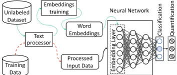
Figure 1 provides a high-level overview of our approach, which consists of two main steps and an optional task-dependent third step: (1) thetext processing, where we use our own text processing tool for preparing the data for our neural network, (2) the learning step, where we train the neural

Unlabeled Dataset

% % %

Training Data

Processed Input Data

C

lassific

at

ion

Qu

ant

if

ic

at

io

n

Embeddings training

Text processor

Neural Network

Word Embeddings

Emb

ed

d

in

g

La

yer

Figure 1: High-level overview of our approach

networks and (3) the quantificationstep for esti-mating the sentiment distribution for each topic.

Task definitions. In Subtask A, given a message we must classify whether the message expresses positive, negative, or neutral sentiment (3-point scale). In Subtasks B, C (topic-based sentiment polarity classification) we are given a message and a topic and must classify the message on 2-point scale (Subtask B) and a 5-point scale (Subtask C). In Subtasks D, E (quantification) we are given a set of messages about a set of topics and must es-timate the distribution of the tweets across 2-point scale (Subtask D) and a 5-point scale (Subtask E).

Unlabeled Dataset. We collected a big dataset of 330M English Twitter messages, gathered from 12/2012 to 07/2016, which is used (1) for calculat-ing words statistics needed by our text processor and (2) for training our word embeddings.

Pre-trained Word Embeddings. Word em-beddings are dense vector representations of words (Collobert and Weston, 2008; Mikolov et al.,2013), capturing their semantic and syntac-tic information. We leverage our big collection of Twitter messages to generate word embeddings, with vocabulary size of 660K words, using GloVe

(Pennington et al., 2014). The pre-trained word

embeddings are used for initializing the first layer (embedding layer) of our neural networks.

2.1 Text Processor

We developed our own text processing tool, in or-der to utilize most of the information in text, per-forming sentiment-aware tokenization, spell cor-rection, word normalization, word segmentation (for splitting hashtags) and word annotation.

Tokenizer. The difficulty in tokenization is to avoid splitting expressions or words that should be kept intact (as one token). Although there

are some tokenizers geared towards Twitter (Potts,

2011;Gimpel et al.,2011) that recognize the Twit-ter markup and some basic sentiment expressions or simple emoticons, our tokenizer is able to iden-tify most emoticons, emojis, expressions such as dates (e.g. 07/11/2011, April 23rd), times (e.g. 4:30pm, 11:00 am), currencies (e.g. $10, 25mil, 50e), acronyms, censored words (e.g. s**t), words with emphasis (e.g. *very*) and more.

Text Postprocessing. After the tokenization we add an extra postprocessing step, performing mod-ifications on the extracted tokens. This is where we perform spell correction, word normalization and segmentation and decide which tokens to omit, normalize or annotate (surround or replace with special tags). For the tasks of spell correction

(Jurafsky and Martin, 2000) and word

segmenta-tion (Segaran and Hammerbacher,2009) we used the Viterbi algorithm, utilizing word statistics (un-igrams and b(un-igrams) from our unlabeled dataset, to obtain word probabilities. Moreover, we low-ercase all words, and normalize URLs, emails and user handles (@user).

After performing the aforementioned steps we decrease the vocabulary size, while keeping infor-mation that is usually lost during the tokenization phase. Table1shows an example of our text pro-cessing pipeline, on a Twitter message.

2.2 Neural Networks

Last year, most of the top scoring systems used Convolutional Neural Networks (CNN) (LeCun

et al.,1998). Even though CNNs are designed for

computer vision, the fact that they are fast and easy to train, makes them a popular choice for NLP problems. However CNNs have no notion of or-der, thus when applying them to NLP tasks the crucial information of the word order is lost.

2.2.1 Recurrent Neural Networks

A more natural choice is to use Recurrent Neu-ral Networks (RNN). An RNN processes an in-put sequentially, in a way that resembles how humans do it. It performs the same operation, ht = fW(xt, ht−1), on every element of a se-quence, wherehtis the hidden state a timestept,

original The *new* season of #TwinPeaks is coming on May 21, 2017. CANT WAIT \o/ !!! #tvseries #davidlynch :D processed the new <emphasis> season of <hashtag> twin peaks </hashtag> is coming on <date> . cant <allcaps> wait

<allcaps> <happy> ! <repeated> <hashtag> tv series </hashtag> <hashtag> david lynch </hashtag> <laugh>

and W the weights of the network. The hidden state at each timestep depends on the previous hid-den states. This is why the order of the elements (words) is important. This process also enables RNNs to handle inputs of variable length.

RNNs are difficult to train (Pascanu et al.,

2013), because gradients may grow or decay expo-nentially over long sequences (Bengio et al.,1994;

Hochreiter et al.,2001). A way to overcome these

problems is by using one of the more sophisti-cated variants of the regular RNN, the Long Short-Term Memory (LSTM) network (Hochreiter and

Schmidhuber, 1997) or the recently proposed

Gated Recurrent Units (GRU) (Cho et al.,2014). Both variants introduce a gating mechanism, en-suring proper gradient propagation through the network. We use the LSTM, as it performed slightly better than GRU in our experiments.

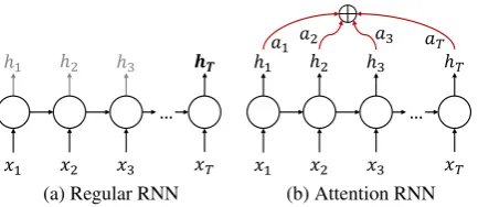
Attention Mechanism. An RNN updates its hid-den statehi as it processes a sequence and at the end, the hidden state holds a summary of all the processed information. In order to amplify the contribution of important elements in the final rep-resentation we use an attention mechanism ( Rock-täschel et al., 2015;Raffel and Ellis, 2015), that aggregates all the hidden states using their relative importance (see Figure2).

𝑥1 ℎ₁

𝑥₂

ℎ₂

𝑥₃

ℎ₃

𝑥_𝑇 𝒉_𝑻

…

(a) Regular RNN

𝑥1

𝑎₁ 𝑎2 𝑎3 𝑎𝑇 ℎ₁

𝑥₂ ℎ₂

𝑥₃ ℎ₃

𝑥_𝑇 ℎ_𝑇

…

(b) Attention RNN

Figure 2: Comparison between the regular RNN and the RNN with attention.

2.3 Quantification

For the quantification tasks an obvious approach is the Classify & Count (Forman, 2008), where we simply compute the fraction of a topic’s messages that a classifier predicts to belong to a class c. Another approach is the Probabilistic Classify & Count (PCC) (Gao and Sebastiani,2016), in which first we train a classifier that produces a probabil-ity distribution over the classes and then we av-erage the estimated probabilities for each class to obtain the final distribution. Let T be the set of topics in the training set andp(c|tweet)the (pos-terior) probability that a tweet belongs to classcas

estimated by the classifier. Then we estimate the expected fraction of a topic’s tweets that belong to classcas follows:

ˆ

pT(c) = _|T1_| X

tweet∈T

p(c|tweet) (1)

3 Models Description

We propose two different models, a Message-level Sentiment Analysis (MSA) model for Subtask A (3.1) and a Topic-based Sentiment Analysis (TSA) (3.2) model for Subtasks B,C,D,E.

3.1 MSA Model (message-level)

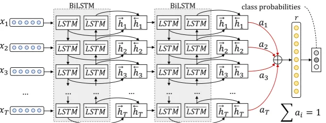
Our message-level sentiment analysis model (MSA) consists of a 2-layer bidirectional LSTM (BiLSTM) with an attention mechanism, for iden-tifying the most informative words.

Embedding Layer. The input to the network is a Twitter message, treated as a sequence of words. We use an Embedding layer to project the words X = (x1, x2, ..., xT) to a low-dimensional vec-tor spaceRE_{, whereEthe size of the Embedding} layer andT the number of words in a tweet. We initialize the weights of the embedding layer with our pre-trained word embeddings.

BiLSTM Layers. An LSTM takes as input the words of a tweet and produces the word annota-tions H = (h1, h2, ..., hT), where hi is the hid-den state of the LSTM at time-step i, summariz-ing all the information of the sentence up to xi. We use bidirectional LSTM (BiLSTM) in order to get word annotations that summarize the informa-tion from both direcinforma-tions. A bidirecinforma-tional LSTM consists of a forward LSTM−→f that reads the sen-tence fromx1toxT and a backward LSTM←f−that reads the sentence fromxT tox1. We obtain the final annotation for a given wordxi, by concate-nating the annotations from both directions:

hi=−→hi k←h−i, hi∈R2L (2)

wherek denotes the concatenation operation and Lthe size of each LSTM. We stack two layers of BiLSTMs in order to learn more abstract features.

𝑥1 𝐿𝑆𝑇𝑀 𝐿𝑆𝑇𝑀 BiLSTM

𝑎1

𝑎𝑇 _{෍ 𝑎𝑖= 1}

ℎ1 ℎ1

𝑥2 𝐿𝑆𝑇𝑀 𝐿𝑆𝑇𝑀 ℎ2 ℎ2

𝑥3 𝐿𝑆𝑇𝑀 𝐿𝑆𝑇𝑀 ℎ3 ℎ3

𝑥𝑇 𝐿𝑆𝑇𝑀 𝐿𝑆𝑇𝑀 ℎ𝑇 ℎ𝑇

… …

𝐿𝑆𝑇𝑀 𝐿𝑆𝑇𝑀 BiLSTM

ℎ1 ℎ1

𝐿𝑆𝑇𝑀 𝐿𝑆𝑇𝑀 ℎ2 ℎ2

𝐿𝑆𝑇𝑀 𝐿𝑆𝑇𝑀 ℎ3 ℎ3

𝐿𝑆𝑇𝑀 𝐿𝑆𝑇𝑀 ℎ𝑇 ℎ𝑇

… …

𝑎2

𝑎3

… … …

classprobabilities

𝑟

Figure 3: The MSA model: A 2-layer bidirectional LSTM with attention over that last layer.

of all the word annotations. Formally:

ei =tanh(Whhi+bh), ei ∈[−1,1] (3)

ai = P_Texp(ei)

t=1exp(et) ,

T

X

i=1

ai = 1 (4)

r=XT

i=1

aihi, r∈R2L (5)

whereWhandbhare the attention layer’s weights, optimized during training to assign bigger weights to the most important words of a sentence.

Output Layer. We use the representationras fea-ture vector for classification and we feed it to a fi-nal fully-connected softmax layer which outputs a probability distribution over all classes.

3.2 TSA Model (topic-based)

For the topic-based sentiment analysis tasks, we propose a Siamese2 _{bidirectional LSTM network}

with a different attention mechanism than in MSA. Our model is comparable to the work of (Wang et al.,2016;Tang et al.,2015). However our model differs in the way it incorporates topic information and in the attention mechanism.

Embedding Layer. The network has two in-puts, the sequence of words in the tweet Xtw ₌

(xtw

1 , xtw2 , ..., xtwTtw), where Ttw the number of

words in the tweet, and the sequence of words in the topicXto _{= (x}to

1, xto2, ..., xtoTto), whereTtothe

number of words in the topic. We project all words toRE_{, whereEthe size of the Embedding layer.}

Siamese BiLSTM. We use a bidirectional LSTM with shared weights to map the words of the tweet and the topic to the same vector space, in order to be able to make meaningful com-parison between the two. The BiLSTM pro-duces the annotations for the words of the tweet 2_{Siamese are called the networks that have identical} con-figuration and their weights are linked during training.

Htw _{= (h}tw

1 , htw2 , ..., htwTtw) and the topicHto =

(hto

1, hto2, ..., htoTto), where each word annotation

consists of the concatenation of its forward and backward annotations:

hj_i =−→hj_i k←h−j_i, hj_i ∈R2L, j∈ {tw, to} (6) wherek denotes the concatenation operation and Lthe size of each LSTM.

Mean-Pooling Layer. We use a Mean-Pooling

layer over the word annotations of the topic Hto that aggregates them to produce a single annota-tion. The layer computes themean over time to produce the topic annotation,hto₌ 1

Tto

P_Tto

1 htoi .

Context-Aware Annotations. We append the topic annotationhto_{to each word annotation to get} the finalcontext-awareannotation for each word:

hi=htw_i khto_{, h}j

i ∈R4L (7)

Context-Attention Layer. We use a context-aware attention mechanism as in (Yang et al.,

2016), in order to strengthen the contribution of words that express sentiment towards a given topic. This is done by adding a context vectoruh that can be interpreted as a fixed query, like “which words express sentiment towards the given topic”, over the words of the message. Concretely:

ei =tanh(Whhi+bh), ei ∈[−1,1] (8)

ai = P_Texp_tw (e>i uh)

t=1exp(e>tuh), Ttw X

i=1

ai= 1 (9)

r =XTtw

i=1

aihi, r∈R4L (10)

whereWh,bhanduhare jointly learned weights.

…

T

w

ee

t

Topic

𝐵𝑖𝐿𝑆𝑇𝑀 𝐵𝑖𝐿𝑆𝑇𝑀

Shared weights

… …

…

𝑀𝑒𝑎𝑛 𝑃𝑜𝑜𝑙𝑖𝑛𝑔

ℎ1𝑡𝑤 ℎ2𝑡𝑤 ℎ3𝑡𝑤 ℎ1𝑡𝑜 ℎ2𝑡𝑜 ℎ3𝑡𝑜

ℎ𝑡𝑜

…

ℎ1𝑡𝑤 ℎ2𝑡𝑤ℎ3𝑡𝑤 ℎ𝑇𝑡𝑤

𝑎1 𝑎𝑇

෍ 𝑎𝑖= 1

𝑎2 𝑎3

M

ax

out

classprobabilities

𝑢ℎ

𝑥1𝑡𝑤 𝑥2𝑡𝑤 𝑥3𝑡𝑤 𝑥𝑇𝑡𝑤

𝑡𝑤 _𝑥

1𝑡𝑜 𝑥2𝑡𝑜 𝑥3𝑡𝑜

𝑟

𝑥𝑇𝑡𝑜

𝑡𝑜

ℎ𝑡𝑤𝑇𝑡𝑤 ℎ𝑇𝑡𝑜

𝑡𝑜

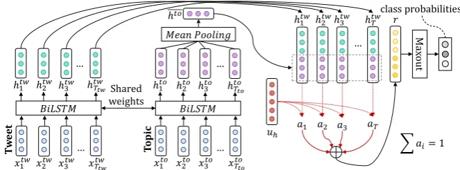
Figure 4: The TSA model: A Siamese Bidirectional LSTM with context-aware attention.

and the topic aspects. We selected Maxout as it amplifies the effects of dropout (Section3.3).

Output Layer. We pass the output of the Max-out layer to a final fully-connected softmax layer which outputs a probability distribution over all classes.

3.3 Regularization

In both of our models we add Gaussian noise at the embedding layer, which can be interpreted as a random data augmentation technique, mak-ing our models more robust to overfittmak-ing. In ad-dition to that, we use dropout (Srivastava et al.,

2014) to randomly turn-off neurons in our net-work. Dropout prevents co-adaptation of neurons and can also be thought as a form of ensemble learning, because for each training example a sub-part of the whole network is trained. Moreover, we apply dropout to the recurrent connections of the LSTM as in (Gal and Ghahramani,2016). Further-more we add L2 regularization penalty (weight decay) to the loss function to discourage large weights. Also, we stop training after the valida-tion loss has stopped decreasing (early-stopping).

Finally, we do not fine-tune the embedding lay-ers. Words occurring in the training set, will be moved in the embedding space and the classifier will correlate certain regions (in embedding space) to certain sentiments. However, words in the test set and not in the training set, will remain at their initial position which may no longer reflect their “true” sentiment, leading to miss-classifications.

3.4 Class Weights

In the training data some classes have more train-ing examples than others, introductrain-ing bias in our models. In order to deal with this problem we ap-ply class weights to the loss function of our mod-els, penalizing more the misclassification of un-derrepresented classes. Moreover, we introduce

a smoothing factor in order to smooth out the weights in cases where the imbalances are very strong, which would otherwise lead to extremely large class weights. Letx be the vector with the class counts and α the smoothing factor, we ob-tain class weights with wi = _xi+max_α×max(x)_(x). In Subtasks A, B, D we use no smoothing (α = 0) and in Subtasks C and E we setα= 0.1.

3.5 Training

We train all of our networks to minimize the cross-entropy loss, using back-propagation with stochastic gradient descent and mini-batches of size 128. We use Adam (Kingma and Ba,2014) for tuning the learning rate and we clip the norm of the gradients (Pascanu et al.,2013) at 5, as an extra safety measure against exploding gradients.

Dataset. For training we use the available data from prior years (only tweets). Table2shows the statistics of the data we used. Also, we do not use any user information from the tweets (only text).

3.5.1 Hyper-parameters

In order to find good hyper-parameter values in a relative short time, compared to grid or ran-dom search, we adopt the Bayesian optimization

(Bergstra et al., 2013) approach, performing a

“smart” search in the high dimensional space of all the possible values.

MSA Model. The size of the embedding layer is 300, and the LSTM layers 150 (300 for BiLSTM). We add Gaussian noise withσ = 0.2and dropout of 0.3 at the embedding layer, dropout of 0.5 at the LSTM layers and dropout of 0.25 at the recur-rent connections of the LSTM. Finally, we addL2 regularization of0.0001at the loss function.

Positive Neutral Negative

Dataset Task 2 1 0 -1 -2 Total

Train A 19652 (39.64%) 22195 (44.78%) 7723 (15.58%) 49570

B,D 14897 (78.85%) - 3997 (21.15%) 18894

C,E 1016 (3.34%) 12852 (42.23%) 12888 (42.35%) 3380 (11.11%) 296 (0.97%) 30432

Test A 2375 (19.33%) 5937 (48.33%) 3972 (32.33%) 12284

B,D 2463 (39.82%) - 3722 (60.18%) 6185

C,E 131 (1.06%) 2332 (18.84%) 6194 (50.04%) 3545 (28.64%) 177 (1.43%) 12379

Table 2: Dataset statistics. Notice the difference in the ratio of positive-negative classes this year.

the embedding layer of the message, dropout of 0.2 at the LSTM layer and the recurrent connec-tion of the LSTM layer and dropout of 0.3 at the attention layer and the Maxout layer. Finally, we addL2regularization of0.001at the loss function.

4 Experiments and Results

Semeval Results. Our official ranking (Rosenthal et al.,2017) is 1/38 (tie) in Subtask A, 2/24 in Sub-task B, 2/16 in SubSub-task C, 2/16 in SubSub-task D and 11/12 in Subtask E. All of our models performed very good, with the exception of Subtask E. Since the quantification was performed on top of the classifier of Subtask C, which came in 2nd _place,

we conclude that our quantification approach was the reason for the bad results for Subtask E.

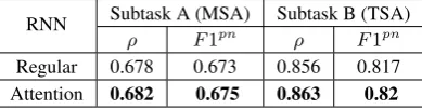
Attention Mechanism. In order to assess the im-pact of the attention mechanisms, we evaluated the performance of each model, with and without at-tention. We report (Table3) the average scores of 10 runs for each system, on the official test set. The attention-based models performed better, but only by a small margin.

RNN Subtask A (MSA) Subtask B (TSA)

ρ F1pn _{ρ F1}pn

Regular 0.678 0.673 0.856 0.817 Attention 0.682 0.675 0.863 0.82

Table 3: Results of the impact of attention3_.

Quantification. To get a better insight into the quantification approaches, we compare the per-formance of CC and PCC. It is inconclusive as to which quantification approach is better. PCC outperformed CC in (Bella et al., 2010) but un-derperformed CC in (Esuli and Sebastiani,2015). Following the results from (Gao and Sebastiani,

2016), which are reported on sentiment analysis in twitter, we decided to use PCC for both of our 3_{ρis the average recall andF1}pn_{the macro-average F1}

score of the positive and negative classes

quantification submissions. Table4shows the per-formance of our models. PCC performed better than CC for Subtask D but far worse than CC for Subtask E. We hypothesize that two possible rea-sons for the difference in performance between D and E, might be (1) the difference in the number of classes and (2) the big change in the ratio ofpos -to-negclasses between the training and test sets.

Method Subtask D Subtask E

KLD AE RAE EMD

CC 0.060 0.093 0.608 0.359

PCC 0.048 0.095 0.848 0.595

Table 4: Results of the quantification approaches4_.

Experimental setup. For developing our mod-els we used Keras (Chollet, 2015) with Theano

(Theano Dev Team,2016) as backend and

Scikit-learn (Pedregosa et al.,2011). We trained our neu-ral networks on a GTX750Ti (4GB). Lastly, we share the source code of our models5_.

5 Conclusion

In this paper, we present two deep-learning sys-tems for short text sentiment analysis developed for SemEval-2017 Task 4 “Sentiment Analysis in Twitter”. We use RNNs, utilizing well established methods in the literature. Additionally, we em-power our networks with two different kinds of at-tention mechanisms in order to amplify the contri-bution of the most important words.

Our models achieved excellent results in the classification tasks, but mixed results in the quan-tification tasks. We would like to work more in this area and explore more quantification techniques in the future. Another interesting approach would be to design models operating on the character-level. 4_{KLD is Kullback-Leibler Divergence,EMDis Earth} Mover’s Distance,AEis Absolute Error andRAEis Rela-tive Absolute Error. For all metrics lower is better.

References

Antonio Bella, Cesar Ferri, José Hernández-Orallo, and Maria Jose Ramirez-Quintana. 2010.

Quantifi-cation via probability estimators. InProceedings of

ICDM. pages 737–742.

Yoshua Bengio, Patrice Simard, and Paolo Frasconi. 1994. Learning long-term dependencies with

gradi-ent descgradi-ent is difficult. IEEE Transactions on

Neu-ral Networks5(2):157–166.

James Bergstra, Daniel Yamins, and David D. Cox. 2013. Making a science of model search: Hyperpa-rameter optimization in hundreds of dimensions for

vision architectures. InProceedings of ICML. pages

115–123.

Kyunghyun Cho, Bart Van Merriënboer, Caglar Gul-cehre, Dzmitry Bahdanau, Fethi Bougares, Holger Schwenk, and Yoshua Bengio. 2014. Learning phrase representations using RNN encoder-decoder

for statistical machine translation. arXiv preprint

arXiv:1406.1078.

Fran¸cois Chollet. 2015. Keras. https://github.

com/fchollet/keras.

Ronan Collobert and Jason Weston. 2008. A unified architecture for natural language processing: Deep

neural networks with multitask learning. In

Pro-ceedings of ICML. pages 160–167.

Jan Deriu, Maurice Gonzenbach, Fatih Uzdilli, Au-rélien Lucchi, Valeria De Luca, and Martin Jaggi. 2016. SwissCheese at SemEval-2016 Task 4: Sen-timent classification using an ensemble of convolu-tional neural networks with distant supervision. In

Proceedings of SemEval. pages 1124–1128. Andrea Esuli and Fabrizio Sebastiani. 2015.

Optimiz-ing Text Quantifiers for Multivariate Loss Functions.

ACM Trans. Knowl. Discov. Data9(4):27:1–27:27. George Forman. 2008. Quantifying counts and costs

via classification. Data Mining and Knowledge

Dis-covery17(2):164–206.

Yarin Gal and Zoubin Ghahramani. 2016. A theoret-ically grounded application of dropout in recurrent

neural networks. In Proceedings of NIPS. pages

1019–1027.

Wei Gao and Fabrizio Sebastiani. 2016. From classifi-cation to quantificlassifi-cation in tweet sentiment analysis.

Social Network Analysis and Mining6(1).

Kevin Gimpel, Nathan Schneider, Brendan O’Connor, Dipanjan Das, Daniel Mills, Jacob Eisenstein, Michael Heilman, Dani Yogatama, Jeffrey Flanigan, and Noah A. Smith. 2011. Part-of-speech tagging for twitter: Annotation, features, and experiments. InProceedings of ACL. pages 42–47.

Ian J. Goodfellow, David Warde-Farley, Mehdi Mirza, Aaron C. Courville, and Yoshua Bengio. 2013.

Maxout networks. InProceedings of ICML. pages

1319–1327.

Sepp Hochreiter, Yoshua Bengio, Paolo Frasconi, and

Jürgen Schmidhuber. 2001. Gradient Flow in

Re-current Nets: The Difficulty of Learning Long-Term Dependencies. A field guide to dynamical recurrent neural networks. IEEE Press.

Sepp Hochreiter and Jürgen Schmidhuber. 1997.

Long short-term memory. Neural Computation

9(8):1735–1780.

Daniel Jurafsky and James H. Martin. 2000. Speech

and Language Processing: An Introduction to Nat-ural Language Processing, Computational Linguis-tics, and Speech Recognition. Prentice Hall PTR, 1st edition.

Diederik Kingma and Jimmy Ba. 2014. Adam: A

method for stochastic optimization. arXiv preprint

arXiv:1412.6980.

Svetlana Kiritchenko, Xiaodan Zhu, and Saif M. Mo-hammad. 2014. Sentiment analysis of short

infor-mal texts. Journal of Artificial Intelligence Research

50:723–762.

Yann LeCun, Léon Bottou, Yoshua Bengio, and Patrick Haffner. 1998. Gradient-based learning applied to

document recognition. Proceedings of the IEEE

86(11):2278–2324.

Tomas Mikolov, Ilya Sutskever, Kai Chen, Greg S. Cor-rado, and Jeff Dean. 2013. Distributed representa-tions of words and phrases and their

compositional-ity. InProceedings of NIPS. pages 3111–3119.

Saif M. Mohammad, Svetlana Kiritchenko, and Xiao-dan Zhu. 2013. NRC-Canada: Building the

state-of-the-art in sentiment analysis of tweets. arXiv

preprint arXiv:1308.6242.

Preslav Nakov, Alan Ritter, Sara Rosenthal, Fabrizio Sebastiani, and Veselin Stoyanov. 2016.

Semeval-2016 Task 4: Sentiment analysis in Twitter. In

Pro-ceedings of SemEval. pages 1–18.

Elisavet Palogiannidi, Athanasia Kolovou, Fenia Christopoulou, Filippos Kokkinos, Elias Iosif, Niko-laos Malandrakis, Haris Papageorgiou, Shrikanth Narayanan, and Alexandros Potamianos. 2016. Tweester at SemEval-2016 Task 4: Sentiment anal-ysis in Twitter using semantic-affective model

adap-tation. InProceedings of SemEval. pages 155–163.

Razvan Pascanu, Tomas Mikolov, and Yoshua Bengio. 2013. On the difficulty of training recurrent

neu-ral networks. InProceedings of ICML. pages 1310–

1318.

Fabian Pedregosa, Gaël Varoquaux, Alexandre Gram-fort, Vincent Michel, Bertrand Thirion, Olivier Grisel, Mathieu Blondel, Peter Prettenhofer, Ron Weiss, Vincent Dubourg, and others. 2011.

Scikit-learn: Machine learning in Python. Journal of

Jeffrey Pennington, Richard Socher, and Christo-pher D. Manning. 2014. Glove: Global Vectors for

Word Representation. In Proceedings of EMNLP.

pages 1532–1543.

Christopher Potts. 2011. Sentiment

Sym-posium Tutorial: Tokenizing. http:

//sentiment.christopherpotts.net/

tokenizing.html.

Colin Raffel and Daniel PW Ellis. 2015.

Feed-forward networks with attention can solve some

long-term memory problems. arXiv preprint

arXiv:1512.08756.

Tim Rocktäschel, Edward Grefenstette, Karl Moritz Hermann, Tomáš Koˇciská˙z¸s, and Phil Blunsom. 2015. Reasoning about entailment with neural

at-tention. arXiv preprint arXiv:1509.06664.

Sara Rosenthal, Noura Farra, and Preslav Nakov. 2017. SemEval-2017 Task 4: Sentiment Analysis in

Twit-ter. InProceedings of SemEval. Vancouver, Canada.

Mickael Rouvier and Benoît Favre. 2016. SENSEI-LIF at SemEval-2016 Task 4: Polarity embedding

fusion for robust sentiment analysis. InProceedings

of SemEval. pages 202–208.

Toby Segaran and Jeff Hammerbacher. 2009. Beautiful

Data: The Stories Behind Elegant Data Solutions. "O’Reilly Media, Inc.".

Nitish Srivastava, Geoffrey E. Hinton, Alex Krizhevsky, Ilya Sutskever, and Ruslan Salakhutdi-nov. 2014. Dropout: A simple way to prevent neural

networks from overfitting. Journal of Machine

Learning Research15(1):1929–1958.

Duyu Tang, Bing Qin, Xiaocheng Feng, and Ting

Liu. 2015. Target-dependent sentiment

classifi-cation with long short term memory. CoRR,

abs/1512.01100.

Theano Dev Team. 2016. Theano: A Python frame-work for fast computation of mathematical

expres-sions. arXiv e-printsabs/1605.02688.

Yequan Wang, Minlie Huang, Xiaoyan Zhu, and Li Zhao. 2016. Attention-based LSTM for

aspect-level sentiment classification. In Proceedings of

EMNLP. pages 606–615.

Zichao Yang, Diyi Yang, Chris Dyer, Xiaodong He, Alex Smola, and Eduard Hovy. 2016. Hierarchical attention networks for document classification. In