Abstract— In the field of probability and statistics, the quantile function and the quantile density function which is the derivative of the quantile function are one of the important ways of characterizing probability distributions and as well, can serve as a viable alternative to the probability mass function or probability density function. The quantile function (QF) and the cumulative distribution function (CDF) of the chi-square distribution do not have closed form representations except at degrees of freedom equals to two and as such researchers devise some methods for their approximations. One of the available methods is the quantile mechanics approach. The paper is focused on using the quantile mechanics approach to obtain the quantile density function and their corresponding quartiles or percentage points. The outcome of the method is second order nonlinear ordinary differential equation (ODE) which was solved using the traditional power series method. The quantile density function was transformed to obtain the respective percentage points (quartiles) which were represented on a table. The results compared favorably with known results at high quartiles. A very clear application of this method will help in modeling and simulation of physical processes.
Index Terms— Quantile, Quantile density function, Quantile mechanics, percentage points, Chi-square, approximation.
I. INTRODUCTION
N statistics, In statistics, quantile function is very important in prescribing probability distributions. It is indispensable in determining the location and spread of any given distribution, especially the median which is resistant to extreme values or outliers [1] [2]. Quantile function is used extensively in the simulation of non-uniform random variables [3] and also can be seen as an alternative to the CDF in analysis of lifetime probability models with heavy tails. Details on and the use of the quantile function in modeling, statistical, reliability and survival analysis can be found in: [4], [5]. It should be noted that probability distributions whose statistical reliability measures do not have a close or explicit form can be conveniently represented through the QF. Chi square distribution is one of such distribution whose CDF
Manuscript received July 16, 2017; revised July 31, 2017. This work was sponsored by Covenant University, Ota, Nigeria.
H. I. Okagbue and T. A. Anake are with the Department of Mathematics, Covenant University, Ota, Nigeria.
[email protected] [email protected]
M.O. Adamu is with the Department of Mathematics, University of Lagos, Akoka, Lagos, Nigeria.
does not have closed form. The search for analytic expression of quantile functions
has been a subject of intense research due to the importance of quantile functions. Several approximations are available in literature which can be categorized into four, namely functional approximations, series expansions; numerical algorithms and closed form written in terms of a quantile function of another probability distribution which can also be refer to quantile normalization.
The use of ordinary differential equations in approximating the quantile has been studied by Ulrich and Watson [6] and Leobacher and Pillichshammer [7]. The series solution to the ordinary differential equations used for the approximation of the quantile function was pioneered by Cornish and Fisher [8], Fisher and Cornish [9] and generalized as Quantile mechanics approach by Steinbrecher and Shaw [10]. The approach was inspired by the works of Hill and Davis [11]. Few researches done on the approximations of the quantile functions of Chi-square distribution were done by [12], [13], [14], [15], [16], [17], [18], [19], [20], [21], [22], [23].
II. FORMULATION
The probability density function of the chi-square distribution and the cumulative distribution function are given by;
1
2 2
2
1
( )
e ,
0,
[0,
)
2
( / 2)
k x
k
f x
x
k
x
k
(1)
,
2 2
( , )
,
2 2
2
k x
k x
F x k
P
k
(2)
where
(.,.)
incomplete gamma functions and(.,.)
P
regularized gamma function.The quantile mechanics (QM) approach was used to obtain the second order nonlinear differential equation. QM is applied to distributions whose CDF is monotone increasing and absolutely continuous. Chi-square distribution is one of such distributions. That is;
1
( )
( )
Q p
F
p
(3) Where the functionF
1( )
p
is the compositional inverse ofQuantile Approximation of the Chi–square
Distribution using the Quantile Mechanics
Hilary I. Okagbue, Member, IAENG, Muminu O. Adamu, Timothy A. Anake
the CDF. Suppose the PDF f(x) is known and the differentiation exists. The first order quantile equation is obtained from the differentiation of equation (3) to obtain;
1
1
1
( )
(
( ))
( ( ))
Q p
F F
p
f Q p
(4) Since the probability density function is the derivative of the cumulative distribution function. The solution to equation (4) is often cumbersome as noted by Ulrich and Watson [6]. This is due to the nonlinearity of terms introduced by the density function f. Some algebraic operations are required to find the solution of equation (4). Moreover, equation (4) can be written as;( ( ))
( ) 1
f Q p Q p
(5) Applying the traditional product rule of differentiation to obtain;2
( )
( ( ))( ( ))
Q p
V Q p
Q p
(6) Where the nonlinear term;( )
d
(ln ( ))
V x
f x
dx
(7)These were the results of [10]. It can be deduced that the further differentiation enables
researchers to apply some known techniques to finding the solution of equation (6).
The reciprocal of the probability density function of the chi-square distribution is transformed as a function of the quantile function.
( ) 1
2 2 2
( )
2 ( ( / 2)) ( )
e
k k Q p
dQ p
k
Q p
dp
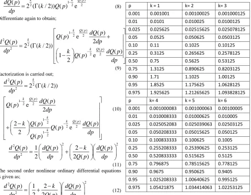
(8)Differentiate again to obtain;
( ) 1
2 2
2
2
2 ( )
2 2
( )
( )
e
2
( )
2 ( ( / 2))
( )
1
( )
e
2
k Q p
k
k Q p
dQ p
Q p
dp
d Q p
k
dp
k
dQ p
Q p
dp
(9) Factorization is carried out;
2
2 2
( ) 1
2 2
1 ( )
2
2 2
1 2
( )
2 ( ( / 2))
( )
( )
e
2
2
( )
( )
( )
e
2
( )
k
k Q p
k
k Q p
k
d Q p
k
dp
dQ p
Q p
dp
k Q p
dQ p
Q p
dp
Q p
(10)
2 2
2
2
( )
1
( )
2
( )
2
2 ( )
d Q p
dQ p
k
dQ p
dp
dp
Q p
dp
(11) The second order nonlinear ordinary differential equations is given as;
2 2
2
( )
1
2
( )
2
2 ( )
d Q p
k
dQ p
dp
Q p
dp
(12)With the boundary conditions;
Q
(0)
0,
Q
(0) 1
.III. POWER SERIES SOLUTION
The cumulative distribution function and its inverse (quantile function) of the chi- square distribution do not have closed form. The power series method was used to find the solution of the Chi-square quantile differential equation (equation (12)) for different degrees of freedom. It was observed that the series solution takes the form of equation (13)
The equations formed a series which can be used to predict p for any given degree of freedom k.
2
1
( )
,
1
4(
1)
Q p
p
p
k
k
(13) For very large k,( )
[image:2.595.52.546.389.771.2]Q p
p
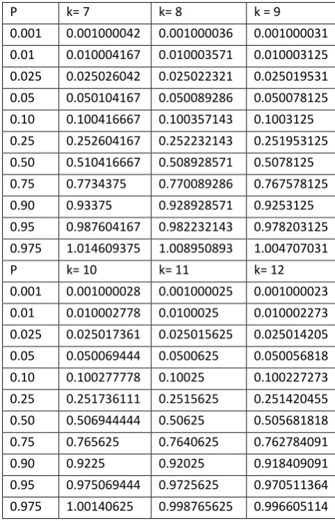
(14) In order to get a very close convergence approximations of the probability p, equation (13) is used for all the degrees of freedom. For examples the values of degrees of freedom from one to twelve is given in Tables 1a and 1b.Table 1a: Quantile density function table for the Chi-square distribution for degrees of freedom from 1 to 6.
p k = 1 k= 2 k= 3
0.001 0.001001 0.00100025 0.001000125 0.01 0.0101 0.010025 0.0100125 0.025 0.025625 0.02515625 0.025078125 0.05 0.0525 0.050625 0.0503125 0.10 0.11 0.1025 0.10125 0.25 0.3125 0.265625 0.2578125 0.50 0.75 0.5625 0.53125 0.75 1.3125 0.890625 0.8203125 0.90 1.71 1.1025 1.00125 0.95 1.8525 1.175625 1.0628125 0.975 1.925625 1.21265625 1.093828125
p k= 4 k = 5 k= 6
Table 1b: Quantile density function table for the Chi-square distribution for degrees of freedom from 7 to 12.
P k= 7 k= 8 k = 9
0.001 0.001000042 0.001000036 0.001000031 0.01 0.010004167 0.010003571 0.010003125 0.025 0.025026042 0.025022321 0.025019531 0.05 0.050104167 0.050089286 0.050078125 0.10 0.100416667 0.100357143 0.1003125 0.25 0.252604167 0.252232143 0.251953125 0.50 0.510416667 0.508928571 0.5078125 0.75 0.7734375 0.770089286 0.767578125 0.90 0.93375 0.928928571 0.9253125 0.95 0.987604167 0.982232143 0.978203125 0.975 1.014609375 1.008950893 1.004707031 P k= 10 k= 11 k= 12 0.001 0.001000028 0.001000025 0.001000023 0.01 0.010002778 0.0100025 0.010002273 0.025 0.025017361 0.025015625 0.025014205 0.05 0.050069444 0.0500625 0.050056818 0.10 0.100277778 0.10025 0.100227273 0.25 0.251736111 0.2515625 0.251420455 0.50 0.506944444 0.50625 0.505681818 0.75 0.765625 0.7640625 0.762784091 0.90 0.9225 0.92025 0.918409091 0.95 0.975069444 0.9725625 0.970511364 0.975 1.00140625 0.998765625 0.996605114
These values are the extent to which the Quantile Mechanics was able to approach the probability.
IV. TRANSFORMATION AND COMPARISON
Transformation to the percentage points and comparison with the exact was done here.
The probability p obtained is transformed using the definition.
Definition Given a probability p which lies between 0 and 1, the percentage points or quartiles or quantile of the chi-square distribution with the non-negative k degrees of freedom is the value
12p( )
k
such that the area under the curve and tothe right of
12p( )
k
is equals to the value 1 – p. The quantile in Table 1 are computed and compared withthe exact values. The readers are refer the r software given as for example
(0.95,3)
[1]7.814728
(0.95, 4)
[2]9.48773
qchisq
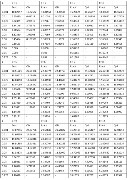
qchisq
The comparisons are presented in Tables 2 for degrees of freedom ranges from 1 to 12. The Quantile mechanics method compares favorably at the following: low probability, high percentage points and higher degrees of freedom. However the methods perform fairly well at the following: high probability, low percentage points and low degrees of freedom.
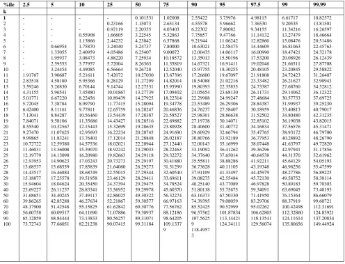
V. PERCENTAGE POINTS FOR THE CHI-SQUARE DISTRIBUTION
The final table for the percentage points or quantile of the chi-square distribution is shown on Table 3. The table of the quantile (percentage points) is quite similar to the one summarized by Goldberg and Levine [24], which includes the results of Fisher [25], Wilson and Hilferty [26], Peiser [27] and Cornish and Fisher [8]. In addition, the result is similar to the works of Thompson [28], Hoaglin [29], Zar [30], Johnson et al. [31] [32] and Ittrich et al. [33].
The same outcome was obtained when compared with the result of Severo and Zelen [15]. This can be seen in Table 4.
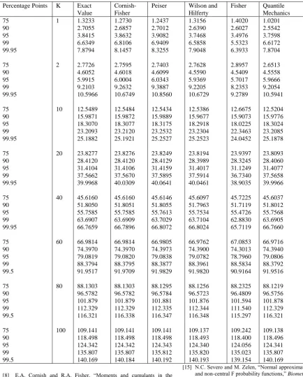
In particular, the QM method performs better at higher percentiles and degrees of freedom when compared with others. The summary is in Table 5.
VI. CONCLUDING REMARKS
The quantile mechanics has been used to obtain the approximations of the percentage points of the chi-square distribution. The method is very efficient at high degrees of freedom, higher percentage points and lower probabilities. However the method performed fairly in the lower degrees of freedom, lower percentiles and high probabilities. This was a part of points noted by [34] that approximation efficiency decreases with the degrees of freedom.
ACKNOWLEDGMENT
The authors are unanimous in appreciation of financial sponsorship from Covenant University. The constructive suggestions of the reviewers are greatly appreciated.
REFERENCES
[1] P.J. Huber, “Robust estimation of a location parameter,” Ann. Math. Stat., vol. 35, no. 1, pp. 73-101, 1964.
[2] F.R. Hampel, “The influence curve and its role in robust estimation,”
J. Amer. Stat. Assoc., vol. 69, no. 346, pp. 383-393, 1974.
[3] W.J. Padgett, “A kernel-type estimator of a quantile function from right-censored data,” J. Amer. Stat. Assoc., vol. 81, no. 393, pp. 215-222, 1986.
[4] E. Parzen, “Nonparametric statistical data modeling,” J. Amer. Stat. Assoc., vol. 74, pp. 105-131. 1979.
[5] N. Reid, “Estimating the median survival time,” Biometrika, vol. 68, pp. 601-608, 1981.
[6] G. Ulrich and L.T. Watson, “A method for computer generation of variates from arbitrary continuous distributions,” SIAM J. Scientific Comp., vol. 8, no. 2, pp. 185–197, 1987.
Table 2: Comparison between the exact and quantile mechanics for degrees of freedom from 1 to 12
p k = 1 k = 2 k = 3 k= 4
Exact QM Exact QM Exact QM Exact QM
0.001 10.82757 10.82572 13.81551 13.81501 16.26624 16.26597 18.46683 18.46664
0.01 6.63490 6.61717 9.21034 9.20535 11.34487 11.34216 13.27670 13.27479
0.025 5.02389 4.98115 7.3776 7.36530 9.34840 9.34155 11.14329 11.14132
0.05 3.84146 3.75976 5.99146 5.96662 7.81473 7.80082 9.48773 9.47766
0.10 2.70554 2.55422 4.60517 4.55578 6.25139 6.22302 7.77944 7.75857
0.25 1.32330 1.02008 2.77259 2.65134 4.10835 4.03403 5.38527 5.32863
0.50 0.45494 0.101531 1.38629 1.15073 2.36597 2.20355 3.35669 3.22545
0.75 0.10153 - 0.57536 0.23166 1.21253 0.92119 1.92256 1.66605
0.90 0.005 - 0.2000 - 0.58437 - 1.06362 0.55908
0.95 0.004 - 0.103 - 0.35185 - 0.71072 -
0.975 0.001 - 0.051 - 0.21580 - 0.48442 -
p k = 5 - k= 6 k = 7 k= 8
Exact QM Exact QM Exact QM Exact QM
0.001 20.51501 20.51486 22.45774 22.45763 24.32189 24.32178 26.12448 26.12439
0.01 15.08627 15.08476 16.81189 16.81063 18.47531 18.47421 20.09024 20.08926
0.025 12.83250 12.82860 14.44938 14.44609 16.01276 16.00990 17.53455 17.53200
0.05 11.07050 11.06242 12.59159 12.58475 14.06714 14.06117 15.50731 15.50196
0.10 9.23636 9.21944 10.64464 10.63021 12.01704 12.00435 13.36157 13.35013
0.25 6.62568 6.57868 7.84080 7.80000 9.03715 9.00072 10.21885 10.18572
0.50 4.35146 4.23842 5.34812 5.24737 6.34581 6.25407 7.34412 7.25934
0.75 2.67460 2.44232 3.45460 3.24040 4.25485 4.05486 5.07064 4.88220
0.90 1.61031 1.13866 2.20413 1.75870 2.83311 2.40959 3.48954 3.08473
0.95 1.14548 - 1.63538 0.66954 2.16735 1.33055 2.73264 1.95937
0.975 0.83121 - 1.23734 - 1.68987 - 2.17973 -
p k = 9 k= 10 k = 11 k= 12
Exact QM Exact QM Exact QM Exact QM
0.001 27.87716 27.87708 29.58830 29.58822 31.26413 31.26407 32.90949 32.90943
0.01 21.66599 21.66511 23.20925 23.20845 24.72497 24.72423 26.21697 26.21627
0.025 19.02277 19.02046 20.48318 20.48105 21.92005 21.91808 23.33666 23.33482
0.05 16.91898 16.91411 18.30704 18.30255 19.67514 19.67097 21.02607 21.02216
0.10 14.68366 14.67321 15.98718 15.97755 17.27501 17.26600 18.54935 18.54088
0.25 11.38875 11.35819 12.54886 12.52040 13.70069 13.67396 14.84540 14.82014
0.50 8.34283 8.26363 9.34182 9.26728 10.34100 10.27030 11.34032 11.27299
0.75 5.89883 5.72004 6.73720 6.56664 7.58414 7.42072 8.43842 8.28129
0.90 4.16816 3.77957 4.86518 4.49085 5.57778 5.21611 6.30380 5.95366
0.95 3.32511 2.59553 3.94030 3.24454 4.57481 3.90687 5.22603 4.58180
Table 3: The percentage points of the Chi-square Distribution
%ile 2.5 5 10 25 50 75 90 95 97.5 99 99.99
k 1 2 3 4 5 6 7 8 9 10 11 12 13 14 15 16 17 18 19 20 21 22 23 24 25 26 27 28 29 30 40 50 60 70 80 90 100 - - - - - - - - - - 1.91767 2.83518 3.59246 4.31155 5.01771 5.72045 6.42400 7.13041 7.84071 8.55540 9.27470 9.99865 10.72722 11.46031 12.19779 12.93953 13.68537 14.43517 15.18877 15.94604 23.69227 31.68651 39.86265 48.17900 56.60758 65.12859 73.72743 - - - - - 0.66954 1.33055 1.95937 2.59553 3.24454 3.90687 4.58180 5.26830 5.96541 6.67220 7.38784 8.11161 8.84287 9.58106 10.32567 11.07625 11.83241 12.59380 13.36008 14.13098 14.90623 15.68559 16.46884 17.25578 18.04624 26.11237 34.40245 42.85288 51.42548 60.09517 68.84444 77.66051 - - - 0.55908 1.13866 1.75870 2.40959 3.08473 3.77957 4.49085 5.21611 5.95366 6.70144 7.45880 8.22456 8.99790 9.77811 10.56460 11.35686 12.15443 12.95693 13.76401 14.57536 15.39070 16.20980 17.03243 17.85839 18.68749 19.51958 20.35450 28.83341 37.49117 46.27634 55.15825 64.11690 73.13833 82.21238 - 0.23166 0.92119 1.66605 2.44232 3.24040 4.05486 4.88220 5.72004 6.56664 7.42072 8.28129 9.14744 10.01867 10.89439 11.77415 12.65759 13.54439 14.43427 15.32699 16.22234 17.12014 18.02021 18.92242 19.82663 20.73273 21.64060 22.55015 23.46129 24.37394 33.56952 42.86025 52.21867 61.62842 71.07886 80.56257 90.07415 0.101531 1.15073 2.20355 3.22545 4.23842 5.24737 6.25407 7.25934 8.26363 9.26728 10.27030 11.27299 12.27531 13.27739 14.27925 15.28094 16.28247 17.28387 18.28516 19.28635 20.28745 21.28848 22.28944 23.29033 24.29118 25.29197 26.29273 27.29344 28.29411 29.29475 39.29978 49.30322 59.30577 69.30776 79.30937 89.31071 99.31184 1.02008 2.65134 4.03403 5.32863 6.57868 7.80000 9.00072 10.18572 11.35819 12.52040 13.67396 14.82014 15.95990 17.09402 18.22314 19.34778 20.46836 21.58527 22.69882 23.80928 24.91690 26.02187 27.12440 28.22463 29.32272 30.41880 31.51299 32.60540 33.69611 34.78524 45.60370 56.32274 66.97163 77.56762 88.12186 98.64205 109.1337 9 2.55422 4.55578 6.22302 7.75857 9.21944 10.63021 12.00435 13.35013 14.67321 15.97755 17.26600 18.54088 19.80393 21.05654 22.29988 23.53489 24.76237 25.98301 27.19738 28.40600 29.60929 30.80766 32.00143 33.19092 34.37640 35.55811 36.73628 37.91109 39.08275 40.25140 51.80118 63.16373 74.39395 85.52425 96.57562 107.5625 9 118.4957 3 3.75976 5.96662 7.80082 9.47766 11.06242 12.58475 14.06117 15.50196 16.91411 18.30255 19.67097 21.02216 22.35835 23.68130 24.99247 26.29306 27.58407 28.86638 30.14071 31.40772 32.66794 33.92189 35.16999 36.41262 37.65014 38.88286 40.11105 41.33497 42.55484 43.77089 55.75675 67.50330 79.08059 90.52999 101.87834 113.14421 124.34111 4.98115 7.36530 9.34155 11.14132 12.82860 14.44609 16.00990 17.53200 19.02046 20.48105 21.91808 23.33482 24.73387 26.11731 27.48684 28.84387 30.18959 31.52502 32.85102 34.16834 35.47765 36.77953 38.07448 39.36296 40.64538 41.92211 43.19348 44.45979 45.72130 46.97828 59.34091 71.41950 83.29706 95.02262 106.62805 118.13541 129.56074 6.61717 9.20535 11.34216 13.27479 15.08476 16.81063 18.47421 20.08926 21.66511 23.20845 24.72423 26.21627 27.68760 29.14062 30.57733 31.99937 33.40813 34.80480 36.19038 37.56576 38.93172 40.28892 41.63797 42.97941 44.31370 45.64129 46.96256 48.27786 49.58752 50.89183 63.69045 76.15364 88.37919 100.42498 112.32860 124.11614 135.80656 10.82572 13.81501 16.26597 18.46664 20.51486 22.45763 24.32178 26.12439 27.87708 29.58822 31.26407 32.90943 34.52812 36.12322 37.69725 39.25230 40.79017 42.31235 43.82015 45.31471 46.79700 48.26790 49.72820 51.17856 52.61962 54.05193 55.47599 56.89225 58.30114 59.70303 73.40193 86.66079 99.60721 112.31691 124.83921 137.20834 149.44924
Table 4: Comparison with known results A
Probability 0.250 0.050 0.005 0.250 0.050 0.005 Percentage points k 75 95 99.95 k 75 95 99.95 Exact Value
Severo and Zelen Quantile Mechanics
Exact Value Severo and Zelen Quantile Mechanics
[image:5.595.40.475.494.662.2]Table 5: Comparison with known results B
Percentage Points K Exact Value
Cornish-Fisher
Peiser Wilson and
Hilferty
Fisher Quantile Mechanics 75 90 95 99 99.95 75 90 95 99 99.95 75 90 95 99 99.95 75 90 95 99 99.95 75 90 95 99 99.95 75 90 95 99 99.5 75 90 95 99 99.5 75 90 95 99 99.5 1 2 10 20 40 60 80 100 1.3233 2.7055 3.8415 6.6349 7.8794 2.7726 4.6052 5.9915 9.2103 10.5966 12.5489 15.9871 18.3070 23.2093 25.1882 23.8277 28.4120 31.4104 37.5662 39.9968 45.6160 51.8050 55.7585 63.6907 66.7659 66.9814 74.3970 79.0819 88.3794 91.9517 88.1303 96.5782 101.879 112.329 116.321 109.141 118.498 124.342 135.807 140.169 1.2730 2.6857 3.8632 6.8106 8.1457 2.7595 4.6018 6.0004 9.2632 10.6749 12.5484 15.9872 18.3077 23.2120 25.1921 23.8276 28.4120 31.4106 37.5670 40.0309 45.6160 51.8051 55.7585 63.6909 66.7896 66.9814 74.3970 79.0820 88.3795 91.9709 88.1303 96.5782 101.879 112.329 116.338 109.141 118.498 124.342 135.807 140.184 1.2437 2.7012 3.9082 6.9409 8.3255 2.7403 4.6099 6.0343 9.3887 10.8560 12.5434 15.9889 18.3175 23.2532 25.2527 23.8249 28.4129 31.4159 37.5895 40.0641 45.6146 51.8055 55.7613 63.7029 66.8072 66.9805 74.3973 79.0838 88.3877 91.9829 88.1295 96.5784 101.881 112.335 116.347 109.141 118.498 124.343 135.812 140.192 1.3156 2.6390 3.7468 6.5858 7.9048 2.7628 4.5590 5.9369 9.2205 10.6729 12.5386 15.9677 18.2918 23.2304 25.2523 23.8194 28.3989 31.4017 37.5914 40.0461 45.6097 51.7963 55.7534 63.7104 66.8024 66.9762 74.3900 79.0782 88.3961 91.9820 88.1256 96.5723 101.876 112.344 116.348 109.137 118.493 124.340 135.820 140.193 1.4020 2.6027 3.4976 5.5323 6.3933 2.8957 4.5409 5.7017 8.2353 9.2789 12.6675 15.9073 18.0225 22.3463 24.0452 23.9397 28.3245 31.1249 36.7340 38.9035 45.7225 51.7119 55.4726 62.8830 65.7119 67.0853 74.3013 78.7960 88.5834 90.9164 88.2325 96.4809 101.594 111.540 115.297 109.242 118.400 124.056 135.023 139.154 1.0201 2.5542 3.7598 6.6172 7.8704 2.6513 4.5558 5.9666 9.2054 10.5941 12.5204 15.9776 18.3024 23.2085 25.1878 23.8093 28.4060 31.4077 37.5658 39.9966 45.6037 51.8012 55.7568 63.6905 66.7660 66.9716 74.3940 79.0806 88.3792 91.9516 88.1219 96.5756 101.878 112.329 116.321 109.138 118.496 124.341 135.807 140.169
[8] E.A. Cornish and R.A. Fisher, “Moments and cumulants in the Specification of Distributions,” Rev. Inter. Stat. Inst., vol. 5, no. 4, pp. 307–320, 1938.
[9] R.A. Fisher and E.A. Cornish, “The percentile points of distributions having known cumulants,” Technometrics, vol. 2, no. 2, pp. 209–225, 1960.
[10] G. Steinbrecher and W.T. Shaw, “Quantile mechanics,” Euro. J. Appl. Math., vol. 19, no. 2, pp. 87-112, 2008.
[11] G.W. Hill and A.W. Davis, “Generalized asymptotic expansions of Cornish-Fisher type,” Ann. Math. Stat., vol. 39, no. 4, pp. 1264–1273, 1968.
[12] M. Merrington, “Numerical approximations to the percentage points of the χ2
distribution,” Biometrika, vol. 32, pp. 200-202, 1941. [13] L.A. Aroian, “A new approximation to the level of significance of the
chi-square distribution,” Ann. Math. Stat., vol. 14, pp. 93-95, 1943. [14] S.H. Abdel-Aty, “Approximate formulae for the percentage points and
the probability integral of the non-central χ 2 distribution,”
Biometrika, vol. 41, no. 3/4, pp. 538-540, 1954.
[15] N.C. Severo and M. Zelen, “Normal approximation to the Chi-square and non-central F probability functions,” Biometrika, vol. 47, pp. 411-416, 1960.
[16] M. Sankaran, “Approximations to the non-central chi-square distribution,” Biometrika, vol. 50, no. 1/2, pp. 199-204, 1963. [17] H.L. Harter, “A new Table of percentage points of the chi-square
distribution,” Biometrika, vol. 51, pp. 231-239, 1964.
[18] R.B. Goldstein, “Algorithm 451: Chi-square Quantiles,” Comm. ACM.
Vol. 16, pp. 483-485, 1973.
[19] D.J. Best and O.E. Roberts, “Algorithm AS 91: The percentage points of the χ2 distribution,” Appl. Stat., vol. 24, pp. 385-388, 1975. [20] M.R. Heyworth, “Approximation to chi-square,” Amer. Statist., vol.
30, pp. 204, 1976.
[21] M.R. Chernick and V.K. Murthy, “Chi-square percentiles: old and new approximations with applications to sample size determination,”
Amer. J. Math. Magt. Sci., vol. 3, no. 2, pp. 145-161, 1983.
[22] J.T. Lin, “Approximating the cumulative chi-square distribution and its inverse,” J. Roy. Stat. Soc. Ser. D., vol. 37, no. 1, pp. 3-5, 1988. [23] J.T. Lin, “New Approximations for the percentage points of the
[24] H. Goldberg and H. Levine, H. (1946). Approximate formulas for the percentage points and normalization of t and χ2. Ann. Math. Stat.,
17(2), 216-225, 1943.
[25] R.A. Fisher, Statistical methods for research workers, Oliver and Boyd, Edinburgh, 1925.
[26] E.B. Wilson and M.M. Hilferly, “The distribution of chi-square”
Proc. Nat. Acad. Sci., vol. 17, pp. 684-688, 1931.
[27] A.M. Peiser, “Asymptotic formulae for significance levels of certain distributions,” Ann. Math. Stat., vol. 14, pp. 56-62, 1943.
[28] C.M. Thompson, “Table of percentage points of the χ2 distribution,”
Biometrika, vol. 32, pp. 188-189, 1941.
[29] D.C. Hoaglin, “Direct approximation for chi-square percentage points,” J. Amer. Stat. Assoc., vol. 72, pp. 508-515, 1977.
[30] J.H. Zar, “Approximations for the percentage points of the chi-square distribution,” J. Roy. Stat. Stat. Soc. Ser. C., vol. 27, no. 3, pp. 280-290, 1978.
[31] N.L. Johnson, S. Kotz and N. Balakrishnan, Continuous Univariate Distributions, Vol 1, Wiley, ISBN: 978-0-471-58495-7, 1994. [32] N.L. Johnson, S. Kotz and N. Balakrishnan, Continuous Univariate
Distributions, Vol 2, Wiley, ISBN: 978-0-471-58494-0, 1995. [33] C. Ittrich, D. Krause and W.D. Richter, “Probabilities and large
quantiles of non-central chi-square distribution,” Statistics, vol. 34, pp. 53-101, 2000.
[34] R.M. Kozelka, “Approximate upper percentage points for extreme values in multinomial sampling”. Ann. Math. Stat., vol. 27, no. 2, pp. 507-512, 1956.