Circumventing Obstacles for Visual Robot
Navigation Using a Stack of Odometric Data
Mateus Mendes
†∗, A. Paulo Coimbra
†, and Manuel M. Cris´ostomo
†Abstract—Recent advances in understanding the source of intelligent behaviour show that it is strongly supported on the use of a large and sophisticated memory. Constant increase of processing power and constant cost decrease of computer memory have encouraged research in vision-based methods for robot navigation. The present approach uses images stored into a Sparse Distributed Memory, implemented in parallel in a Graphics Processing Unit, as a method for robot localization and navigation. Algorithms for following previously learnt paths using visual and odometric information are described. A stack-based method for avoiding random obstacles, using visual information, is proposed. The results show the algorithms are adequate for indoors robot localization and navigation.
Index Terms—Autonomous Navigation, View-Based Naviga-tion, Obstacle Avoidance, View-based LocalizaNaviga-tion, SDM.
I. INTRODUCTION
D
EVELOPMENT of intelligent robots is an area of intense and accelerating research. Different models for localization and navigation have been proposed. The present approach uses a parallel implementation of a Sparse Distributed Memory (SDM) as the support for vision and memory-based robot localization and navigation. The SDM is a type of associative memory suitable to work with high-dimensional Boolean vectors. It was proposed in the 1980s by P. Kanerva [1] and has successfully been used before for based robot navigation [2], [3]. Simple vision-based methods, such as implemented by Matsumoto [4], although sufficient for many environments, in monotonous environments such as corridors may present a large number of errors.The robot learns new paths during a supervised learning stage. While learning, the robot captures views of the sur-rounding environment and stores them in the SDM, along with some odometric and additional information. During autonomous navigation, the robot captures updated views and uses the memory’s algorithms to search for the closest image, using the retrieved image’s additional information as basis for localization and navigation. Memory search is performed in parallel in a Graphics Processing Unit (GPU). Still during the autonomous navigation mode, the environment is scanned using sonar and infra-red sensors (IR). If obstacles are detected in the robot’s path, an obstacle-avoidance algorithm takes control of navigation until the obstacle is overcome. In straight paths, the algorithm creates a stack of odometric data that is used later to return to the original heading. Afterward, vision-based navigation is resumed.
∗ESTGOH, Polytechnic Institute of Coimbra, Portugal. E-mail:
†ISR - Institute of Systems and Robotics, Dept. of Electrical and
Computer Engineering, University of Coimbra, Portugal. E-mail: [email protected], [email protected].
Section II briefly describes the SDM. Section III presents the key features of the experimental platform used. The prin-ciples for vision–based navigation are explained in Section IV. Section V describes two of the navigation algorithms implemented in the robot. It also presents the results of the tests performed with those algorithms. In Section VI, the obstacle avoidance algorithms are described, along with the validation tests and results. Conclusions and future work are presented in Section VII.
II. SPARSEDISTRIBUTEDMEMORY
The properties of the SDM are inherited from the prop-erties of high-dimensional binary spaces, as originally de-scribed by P. Kanerva [1]. Kanerva proves that high-dimensional binary spaces exhibit properties in many aspects related to those of the human brain, such as naturally learning (one-short learning, reinforcement of an idea), naturally forgetting over time, ability to work with incomplete infor-mation and large tolerance to noisy data.
A. Model of the original SDM
Fig. 1 shows a minimalist example of the original SDM model. The main structures are an array of addresses and an array of data counters. The memory is sparse, in the sense that it contains only a fraction of the locations of the addressable space. The locations which physically exist are called hard locations. Each input address activates all the hard locations which are within a predefined access radius (3 bits in the example). The distance between the input address and each SDM location is computed using the Hamming distance, which is the number of bits in which two binary numbers are different. Data are stored in the bit counters. Each location contains one bit counter for each bit of the input datum. To write a datum in the memory, the bit counters of the selected locations will be decremented where the input datum is zero and incremented where the input datum is one. Reading is performed by sampling the active locations. The average of the values of the bit counters is computed column-wise for each bit, and if the value is above a given threshold, a one is retrieved. Otherwise, a zero is retrieved. Therefore, the retrieved vector may not be exactly equal to the stored vector, but Kanerva proves that most of the times it is.
B. Simplified SDM model
Fig. 1. Diagram of a SDM, according to the original model, showing an array of bit counters to store data and an array of addresses. Memory locations within a certain radius of the reference address are selected to read or write.
Fig. 2. Arithmetic SDM model, which operates using integer values.
natural binary code are sensitive to the positional value of the bits and that negatively affects the performance of the system [5]. In order to overcome some of the drawbacks described, other SDM models have been proposed [5], [6], [7]. Fig. 2 shows a model based on Ratitch et al.’s approach [6], which groups data bits as integers and uses the sum of absolute differences instead of the Hamming distance to compute the distance between an input address and location addresses in the memory. That has been the model used in the present work. It was named “arithmetic SDM” and its performance has been superior to the original model [8].
C. SDM parallel implementation in a GPU
The SDM model was implemented first in a CPU, using linked lists as depicted in the upper part of Fig. 3. As the volume of data available to process in real time increased, it became clear that the system could benefit from a parallel implementation of the search procedure. The SDM was then implemented in parallel, in a GPU, using CUDA architecture, as shown in the lower part of Fig. 3. During the learning stage of the robot, the linked list is built using only the CPU and central RAM memory. When learning is over, the list contents are copied to an array of addresses and an array of data in the GPU memory. Later, when necessary to retrieve any information from the SDM, multiple GPU kernels are launched in parallel to check all memory locations and get a quick prediction. The parallel implementation is described in more detail in [9].
III. EXPERIMENTALPLATFORM
The experimental platform consists of a mobile robot carrying a laptop running the control and interface software.
A. Hardware
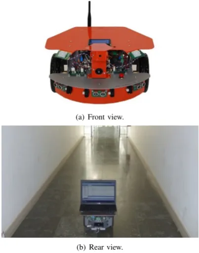
The robot used was an X80Pro11, as shown in Fig. 4. It is a differential drive vehicle equipped with two driven wheels,
[image:2.595.110.226.196.290.2]1From Dr Robot Inc., www.drrobot.com.
Fig. 3. Block diagram of the SDM implemented in the CPU and in the GPU.
(a) Front view.
(b) Rear view.
Fig. 4. Pictures of the robot used, (a) standing alone and (b) with the control laptop, while executing a mission.
each with a DC motor, and a rear swivel caster wheel, for stability. The robot has a built-in digital video camera, an integrated WiFi system (802.11g), and offers the possibility of communication by USB or serial port. For additional support to obstacle avoidance it has six ultrasound sensors (three facing forward and three facing back) and seven infra-red sensors with a sensing range of respectively 2.55 m and 0.80 m.
The robot was controlled in real time from a laptop with a 2.40 GHz Intel Core i7 processor, 6 Gb RAM and a NVIDIA GPU with 2 Gb memory and 96 CUDA cores.
B. Software
[image:2.595.325.527.210.466.2]Fig. 5. Interactions between software modules and the robot.
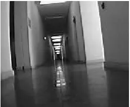
Fig. 6. Example of a picture captured by the robot’s camera, converted to PGM.
IV. VISION-BASED NAVIGATION
Robot localization and navigation are based on visual memories, which are stored into the SDM during a learning stage and later used in the autonomous run mode.
A. Supervised learning
During the supervised learning stage, the user drives the robot along a path using the mouse as input device. During this process, the robot acquires pictures in BMP format with 176 ×144 resolution, which are converted to PGM format. Each recorded image is saved in the disk, along with navigation data, and later stored into the SDM. Fig. 6 shows an image as captured by the robot. Each path has a unique sequence number and is described by a sequence of views, where each view is also assigned a unique view number. Hence, the images are used as addresses for the SDM and the navigation data vectors stored into the SDM are in the following format: < seq#, im#, vr, vl > The sequence number is seq#. The number of the image in the sequence isim#. The velocities of the right and left wheels are, respectively,vrandvl.
B. Autonomous navigation and drift correction
For the autonomous run mode, the user first chooses the destination among the set of previously learnt paths. The robot starts by capturing an image that is converted to PGM and filtered to improve its quality [10]. Then, it is sent to the SDM to be compared with the images in the memory. The SDM returns the image ranked as the most similar to the captured image. After obtaining the image which is closest to its current view, the information associated with that retrieved image (left and right wheel velocities) is used to reproduce the motion performed at the time the image was captured and stored during the learning stage.
Since the robot is following the paths by following the same commands executed during the learning stage, small drifts inevitably occur and accumulate over time. In order to prevent those drifts from accumulating a large error, a correc-tion algorithm was also implemented, following Matsumoto et al.’s approach [11], [4]. Once an image has been predicted, a block-matching method is used to determine the horizontal drift between the robot’s current view and the view retrieved from the memory which was stored during the learning stage. If a relevant drift is found, the robot’s heading is adjusted by proportionally decreasingvrorvl, in order to compensate the lateral drift.
C. Sequence disambiguation
During the autonomous run mode, the data associated with each image that is retrieved from the memory is checked to determine if the image belongs to the sequence (path) that is being followed. Under normal circumstances, the robot is not expected to skip from one sequence to another. Nonetheless, under exceptional circumstances it may happen that the robot is actually moved from one path to another, for unknown reasons. Possible reasons include slippage, manual displacement, mismatch of the original location, among many others. Such problem is commonly known as the “kidnapped robot,” for it is like the robot is kidnapped from one point and abandoned at another point, which can be known or unknown.
To deal with the “kidnapped robot” problem and similar difficulties, the robot uses a short term memory ofnentries (50 was used in the experiments). This short term memory is used to store up tonof the last sequence numberSj that
were retrieved from the memory. If the robot is following sequenceSj, thenSj should always be the most popular in
the short term memory. If an image from sequence Sk is
retrieved, it is ignored, and another image is retrieved from the SDM, narrowing the search to just entries of sequenceSj.
Nonetheless,Sk is still pushed onto the short term memory,
and if at some pointSk becomes more popular in the short
term memory thanSj, the robot’s probable location will be
updated toSk. This disambiguation method showed to filter
out many spurious predictions while still solving kidnapped robot-like problems.
D. Use of a sliding window
When the robot is following a path, it is also expected to retrieve images only within a limited range. For example, if it is at the middle of a long path, it is not expected to get back to the beginning or right to the end of the path. Therefore, the search space can be truncated to a moving “sliding window,” within the sequence that is being followed. For a sequence containing a total ofzimages, using a sliding window of widthw, the search space for the SDM at image imk is limited to images with image number in the interval
{max(0, k −w
2), min(k+ w
[image:3.595.105.234.198.304.2]implementation, however, the selected coordinates are used just to select a subset of the whole space. The subset is then used for computing the distance using all the coordinates.
The sliding window may prevent the robot from solving the kidnapped robot problem. To overcome the limitation, an all-memory search is performed first and the short-term memory retains whether the last n images were predicted within the sliding window or not, as described in Section IV-C. This means that the sliding window actually does not decrease the total search time, since an all-memory search is still required in order to solve the kidnapped robot problem. The sliding window, however, greatly reduces the number of Momentary Localisation Errors (MLE). A momentary localisation error is counted when the robot retrieves from the memory a wrong image, such as an image from a wrong sequence or from the wrong place in the same sequence. When a limited number of MLE occur the robot does not get lost, due to the use of the sliding window and the sequence disambiguation procedures, as described in [10].
V. COMPARISON OF NAVIGATION ALGORITHMS
Different navigation algorithms were implemented and tested. The two most relevant of them are described in the following subsections: the simplest and the most robust.
A. Basic algorithm
The first navigation algorithm is called “basic,” for it performs just the simplest search and navigation tasks, as described in Sections IV-B and IV-C above, and a very basic filtering technique to filter out possibly wrong predictions, described next.
Image search, for robot localisation, is performed in all the memory. Its performance is evaluated counting the number of MLEs. Detection of possible MLEs is based on the number of the image, balanced by the total size of the sequence. If the distance between image imt, predicted at time t, and
imageimt±1, predicted at timet±1, is more than 13z, for a path described byz images,imt±1 is ignored and the robot continues performing the same motion it was doing before the prediction. The fraction 13zwas empirically found for the basic algorithm.
The performance of this basic algorithm was tested indoors in the corridors of the Institute of Systems and Robotics of the University of Coimbra, Portugal. The robot was taught a path about 22 meters long, from a laboratory to an office, and then instructed to follow that path 5 times. Fig. 7 shows the sequence numbers of the images that were taught and retrieved each time. The robot never got lost and always reached a point very close to the goal point.
In a second test, the robot was taught a path about 47 meters long. The results are shown in Fig. 8. As the figure shows, the robot was not able to reach the goal, it got lost at about the 810th prediction in the first run and at the 520th in the second run.
[image:4.595.307.546.51.172.2]The results obtained in the second test show that the basic algorithm is not robust enough, at least for navigating in long and monotonous environments such as corridors in the interior of large buildings.
Fig. 7. Image sequence numbers of the images predicted by the SDM following the path from a laboratory to an office (approx. 22 m). The graph shows the number of the images that are retrieved from the memory as the robot progresses towards the goal.
Fig. 8. Images predicted by the SDM following the second test path (approx. 47 m) using the basic algorithm.
B. Improved autonomous navigation with sliding window
Many of the prediction errors happen where the images are poor in patterns and there are many similar views in the same path or other paths also stored in the memory. Corridors, for example, are very monotonous and thus prone to prediction errors, because a large number of images taken in different places actually have a large degree of similarity. The use of a sliding window to narrow the acceptable predictions improves the results. The improved sliding window algorithm with the other principles described in Section IV-D worked in all situations that it was tested.
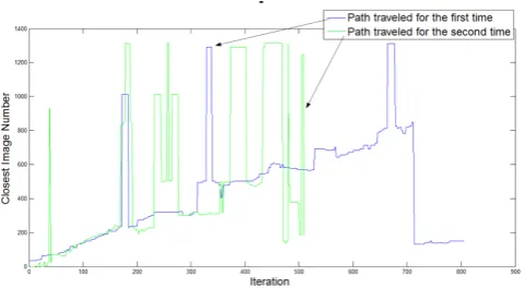
Fig. 9 shows the result obtained with this navigation algorithm when the robot was made to follow the same path used for Fig. 8 (second test path), with a sliding window 40 images wide. As the graph shows, the sliding window filters out all the spurious predictions which could otherwise compromise the ability of the robot to reach the goal. Close to iterations number 200 and 1300, some of the most similar images retrieved from the memory are out of the sliding window, but those images were not used for retrieving control information because they were out of the sliding window. This shows the use of the sliding window correctly filtered wrong predictions out and conferred stability to the navigation process.
VI. OBSTACLEAVOIDANCE
[image:4.595.306.546.230.362.2]Fig. 9. Images predicted by the SDM following the second test path using the sliding window algorithm.
which appear in straight line paths and another for obstacles that appear in curves.
A. Obstacles in straight paths
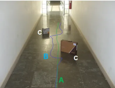
In the autonomous navigation mode, the front sonar sen-sors are activated. All objects that are detected at less than 1 m from the robot are considered obstacles and trigger the obstacle avoidance algorithm. A median of 3 filter was implemented to filter out possible outliers in the sonar readings. When an obstacle is detected, the robot suspends memory-based navigation and changes direction to the side of the obstacle that seems more free. The robot chooses the side by reading the two lateral front sonar sensors. The side of the sensor that gives the higher distance to an object is considered the best side to go. If both sensors read less than 50 cm the robot stops to guarantee its safety. Providing the robot senses enough space, it starts circumventing the obstacle by the safest side. While circumventing, it logs the wheel movements in a stack. When the obstacle is no longer detected by the sensors, the wheel movements logged are then performed in reverse order emptying the stack. This process returns the robot to its original heading. When the stack is emptied, the robot tries to localize itself again based on visual memories and resume memory-based navigation. If the robot cannot localise itself after the stack is empty, then it assumes it is lost and navigation is stopped. In the future this behaviour may be improved to an active search method. Fig. 10 shows an example of a straight path previously taught and later followed with two obstacles placed in that path. After avoiding collision with the first obstacle, the robot resumes memory-based navigation maintaining its original heading, performing lateral drift correction for a while. It then detects and avoids the second obstacle and later resumes memory-based navigation maintaining its original heading. Note that in the figure, because the lines were drawn using a pen attached to the rear of the robot, when the robot turns to the left it draws an arc of a line to the right.
B. Obstacles in curves
[image:5.595.49.290.57.177.2]The stack method described in the previous subsection works correctly if the obstacle is detected when the robot is navigating in a straight line. If the obstacle is detected while the robot is performing a curve, that method may not work, because the expected robot’s heading after circumventing the obstacle cannot be determined in advance with a high degree of certainty. If an obstacle is detected when the robot is
Fig. 10. Examples of obstacle avoidance in a straight path (the lines were drawn using a pen attached to the rear of the robot, so they actually mark the motion of its rear, not its centre of mass). A) Path followed without obstacles. B) Path followed with obstacles. C) Obstacles.
Fig. 11. Examples of obstacle avoidance in a curve. A) Path taught. B) Path followed by the robot avoiding the obstacle D and the left wall corner. C) Path followed by the robot when the obstacle was positioned at D’.
changing its heading, then the stack method is not used. The robot still circumvents the obstacle choosing the clearer side of the obstacle. But in that case it only keeps record of which side was chosen to circumvent the obstacle and what was the previous heading. Then, when the obstacle is no longer detected, the robot uses vision to localise itself and fine tune the drift using the algorithm described in Section IV-B. In curves, the probability of confusion of images is not very high, even if the images are captured at different distances. The heading of the camera often has a more important impact on the image than the distance to the objects. Therefore, after the robot has circumvented the obstacle it will have a very high probability of being close to the correct path and still at a point where it will be able to localise itself and determine the right direction to follow.
Fig. 11 shows examples where the robot avoided obstacles placed in a curve. In path B (blue) the wall corner at the left is also detected as an obstacle, hence there is actually a second heading adjustment. The image shows the robot was still able to localise itself after the obstacle and proceed in the right direction, effectively getting back to the right path.
VII. CONCLUSION
[image:5.595.327.525.260.406.2]implemented in parallel in a GPU for better performance. The use of a stack to store the robot motions when circum-venting obstacles showed good performance in straight paths. For curves, after circumventing the obstacle the robot adjusts its heading faster using only memory-based navigation for localization and the drift-correction algorithm for heading adjustment.
Experimental results show the method was effective for navigation in corridors, even with corners.
Future work will include development of higher level mod-ules to implement behaviours such as wandering, advanced surveillance and cicerone behaviors in the robot.
Acknowledgment
Research supported in part by POCI-01-0145-FEDER-006906.
REFERENCES
[1] P. Kanerva, Sparse Distributed Memory. Cambridge: MIT Press, 1988.
[2] M. Mendes, A. P. Coimbra, and M. M. Cris´ostomo, “Robot navigation based on view sequences stored in a sparse distributed memory,”
Robotica, July 2011.
[3] R. P. N. Rao and D. H. Ballard, “Object indexing using an iconic sparse distributed memory,” The University of Rochester, Computer Science Department, Rochester, New York, Tech. Rep. 559, July 1995. [4] Y. Matsumoto, K. Ikeda, M. Inaba, and H. Inoue, “Exploration and
map acquisition for view-based navigation in corridor environment,” inProceedings of the International Conference on Field and Service Robotics, 1999, pp. 341–346.
[5] M. Mendes, M. M. Cris´ostomo, and A. P. Coimbra, “Assessing a sparse distributed memory using different encoding methods,” inProc. of the World Congress on Engineering (WCE), London, UK, July 2009. [6] B. Ratitch and D. Precup, “Sparse distributed memories for on-line
value-based reinforcement learning.” inECML, 2004.
[7] J. Snaider, S. Franklin, S. Strain, and E. O. George, “Integer sparse distributed memory: Analysis and results,”Neural Networks, no. 46, pp. 144–153, 2013.
[8] M. Mendes, A. P. Coimbra, and M. M. Cris´ostomo, “Intelligent robot navigation using view sequences and a sparse distributed memory,”
Paladyn Journal of Behavioural Robotics, vol. 1, no. 4, April 2011. [9] A. Rodrigues, A. Brand˜ao, M. Mendes, A. P. Coimbra, F. Barros,
and M. Cris´ostomo, “Parallel implementation of a sdm for vision-based robot navigation,” in13th Spanish-Portuguese Conference on Electrical Engineering (13CHLIE), Valˆencia, Spain, 2013.
[10] M. Mendes, A. P. Coimbra, and M. M. Cris´ostomo, “Improved vision-based robot navigation using a sdm and sliding window search,”
Engineering Letters, vol. 19, no. 4, November 2011.
[11] M. Mendes, M. M. Cris´ostomo, and A. P. Coimbra, “Robot navigation using a sparse distributed memory,” inProc. of IEEE Int. Conf. on Robotics and Automation, Pasadena, California, USA, May 2008. [12] L. A. Jaeckel, “An alternative design for a sparse distributed memory,”