A Comparative Study of SISO Control for TITO
Systems
Yusuf Sha’aban,
Member, IAENG,
Abdullahi Muhammad, Kabir Ahmad, and Muazu Jibrin,
Member, IAENG
Abstract—This paper presents a decentralised model predic-tive control (DMPC) for two-input and two-output (TITO) pro-cesses. To reduce the computational load, shifted input sequence is used to cater for loop interactions. The proposed scheme is applied to a coupled system to demonstrate the performance the DMPC. Model predictive control (MPC) and decentralised PID (PI) were also applied for comparison purposes.
Index Terms—decentralised control; decoupling; TITO pro-cess; FOPDT; MPC.
I. INTRODUCTION
T
WO-input and two-output (TITO) systems form a large class of industrial multi-variable systems. Most of such systems are characterised by loop coupling and interactions; making the design of efficient controllers challenging. PID controllers are the most popular in the industry; accounting for over 80% of all industrial controllers [1] . MPC is the only advanced control strategy that has had impact on the industry [2]. These PID controllers are either implemented in a multi-loop fashion or in a decentralised fashion using decouplers. The tuning of multi-loop PID is challenging; the loops cannot be tuned independently, so controllers are loosely tuned to ensure system stability [3], [4]. This leads to inefficient performance. The decentralised PID is more tightly tuned; the use of decouplers allows for SISO design. Much research has been done in both multi-variable and decentralised PID controllers [5], [6], [7].The use of MPC is another way of dealing with loop interactions systematically. On multi-variable systems, MPC is traditionally implemented as a multi-variable control strategy. However, the difficulty in control of large scale and networked systems has led to development of decen-tralised/distributed MPC (DMPC) mainly to mitigate the difficulty associated with maintenance. Most existing indus-trial control loops are already configured in a SISO format. As such practitioners are generally more comfortable with SISO design. Exploring the deployment of DMPC on TITO systems may motivate more implementation of MPC on loops in which benefits are possible. There has been so much interest recently in the area of DMPC for large scale and networked systems [8], [9], [10].
The purpose of this paper is to propose a decentralised MPC scheme for TITO systems and then compare its per-formance with multi-variable PID, decentralized PID, and traditional MPC. The paper is therefore organised as follows:
Manuscript received March 18, 2013; revised April 04, 2013.
Yusuf Sha’aban is with the Department of Electrical and Computer Engineering, Ahmadu Bello University, Zaria, Nigeria. Currently doing a PhD at the University of Manchester, UK : (email:[email protected]; [email protected]).
A. Muhammad, K. Ahmad and M. Jibrin are with the Department of Electrical and Computer Engineering, Ahmadu Bello University, Zaria, Nigeria.
Model predictive control and our formulation of decentral-ized MPC for TITO systems is presented in section II. Two decentralised PID formulations are presented in section III. The simulation results are given in section IV and the paper is concluded in section V.
II. MPCANDDECENTRALISEDMPC
Condiser a TITO process described by (1)
G(s) =
g11(s)e−sθ11 g12(s)e−sθ12
g21(s)e−sθ21 g22(s)e−sθ22
(1)
where
g11(s) =
K11
τ11s+ 1
g12(s) =
K12
τ12s+ 1
g21(s) =
K21
τ21s+ 1
g22(s) =
K22
sτ22s+ 1
A. Model Predictive Control
Model predictive control is a matured technology with most recent research focused on the state space formulation. Different state space formulations exist [11], [12]. In this paper, the formulation in [12] will be used. The model given in (1) can be converted to discrete state space format and the augmented velocity format (2) and (3) respectively [12]:
xp(k+ 1) =Apxp(k) +Bpu(k)
yp(k) =Cpxp(k) (2)
x(k+ 1) =Ax(k) +B∆u(k)
y(k) =Cx(k) (3)
Where
A=
Ap 0Tn CpAp I
; B =
Bp CpBp
C=
0np Inout
; x(k)T =
∆xp(k)T yp(k)T
∆xp(k) =xp(k)−xp(k−1)
Considering the effects of measured disturbanced(k), (2) and (3) become (4) and (5) respectively:
xp(k+ 1) =Apxp(k) +Bpu(k) +Bdd(k)
yp(k) =Cpxp(k) (4)
x(k+ 1) =Ax(k) +B∆u(k) +BD∆d(k)
y(k) =Cx(k) (5)
Where
Bd=
Bp CpBp
One of the formulation of the cost function which penalizes the tracking error as well as the change in control manipu-lated variable is:
J =
p
X
i=1
kr(k+ 1)−y(k+i)k2
q+ M
X
i=1 k∆uk2
rw (6)
If we denotex(k1)byx0, and define the vectors:
XT =
x(k+ 1)T x(k+ 2)T . . . x(k+N p)T
∆UT =∆u(k)T . . . ∆u(k+N c−1)T
YT =y(k+ 1)T y(k+ 2)T . . . y(k+Np)T
(7)
With∆D defined in a similar manner as∆U, the prediction equations can be written in compact form as:
X =F1x0+ Φ1∆U + Φd1∆D
Y =CF1x0+CΦ1∆U+CΦd1∆D
=F x0+ Φ∆U+ Φd∆D (8)
where
FT =
(CA)T (CA2)T . . . (CAP)T
Φ =
CB 0 . . . 0
CAB CB . . . 0
.. .
CAP−1B CAP−2B . . . CAP−MB
The matrix Φd is obtained by substituting B = Bd in the
definition of Φ. The cost function (6) can be written in compact form as:
J = (S−Y)TQ¯(S−Y) + ∆UTR¯∆U (9)
where:
ST =1 1 . . . 1
r(k)
¯
Q > 0 ∈ RpP×pP is a block diagonal output weighting
matrix.R¯ ≥0is a block diagonal input weighting matrix. Substituting (8) in (9) gives an expression for the cost function. The optimal unconstrained control trajectory is then obtained by differentiating the cost function and equating to zero:
∆U =− ΦTQ¯Φ +R−1ΦTQ¯(F x0+ Φd∆D−S) (10)
The constraints can also be written in compact form as:
M∆U ≤N
The the constrained MPC problem can be written as: Minimise:
J = ∆UT ΦTQ¯Φ +R∆U+ 2∆UTΦTQ¯Γ
+constant
subject to the constraints:M∆U ≤N (11)
where
Γ =F x0+ Φd∆D−S
B. Decentralised Model Predictive Control
The process G(s) in (1) can be partitioned into two subsystems:
G1(s) =
g11(s)e−τ11(s) g12(s)e−τ12(s)
G2(s) =
g21(s)e−τ21(s) g22(s)e−τ22(s)
(12)
The sub-systems in (12) can then be converted in to discrete state space format with the second input as a measured disturbance and first input as a measured disturbance in the first and second subsystems respectively. The subsystems represented by (13) are only coupled through the inputs i.e. state couplings do not exist. Moreover it is always possible to bring any system to this format [8].
xpi(k+ 1) =Apixpi(k) +Bpiui(k) +Bdiuj(k)
yi(k) =cpixpi
i, j= 1,2, i6=j (13)
The velocity augmented form model as formulated in (3) can then be formed as:
xi(k+ 1) =Aixi(k) +Bi∆ui(k) +BDi∆udj(k)
yi(k) =Cix(k) (14)
The prediction equations then become:
Xi =F1ixi0+ Φ1i∆Ui+ Φdi∆Di (15)
Yi =Fixi0+ Φi∆Ui+ ΦDi∆Di (16)
With all parameters defined as in section II-A,
Φdi,ΦDi and∆Di defined as follows:
∆Di=
∆uj(k)
∆uj(k+ 1)
.. .
∆uj(k+M −1)
(17)
The prediction equation and MPC laws for each of the sub-systems can be derived as shown in II-A by substituting∆u2 and∆u1as disturbances in subsystems 1 and 2 respectively. To prevent iteration as with traditional distributed MPC, we define the trajectory computed at sampling stepkas:
∆ ˆDi(k) =
∆ ˆuj(k)
∆ ˆuj(k+ 1)
.. .
∆ ˆuj(k+M −1)
(18)
Then since at sampling stepk+ 1,∆ ˆDi for i= 1,2will not
be available, so we will assume that the value computed at
kis still optimal. Hence, we shift the sequence and then add the value at the end of the control horizon i.e.
∆ ˆDi(k+ 1) =
∆ ˆuj(k+ 1)
.. .
∆ ˆuj(k+M −2)
∆ ˆuj(k+M −1)
∆ ˆuj(k+M −1)
(19)
So that (16) is written as:
Yi=Fixi0+ Φi∆Ui+ ΦDi∆ ˆDi(k) (20)
Minimise
Ji= ∆UiT Φ T
iQ¯iΦi+Ri∆Ui+ 2∆UiTΦ T iQ¯iΓi
+constant
subject to the constraints:Mi∆Ui≤Ni:i= 1,2 (21)
where
Γi=Fixi0+ ΦDi∆ ˆDi−S
In this formulation, iteration is not required as in other DMPC implementations. This will reduce the computational and convergence requirements of other decentralised MPC formulations.
III. DECENTRALISEDPID
Consider the system model defined by (1), two decen-tralised PID/PI controllers are presented. The detailed study of the controllers and decouplers presented here are given in [13] and [4].
A. PID with Lead-Lag Decoupler (Wang-PID)
In [13], an auto tuned PID was presented; a clear descrip-tion of the identificadescrip-tion, control design and auto-tuning was presented. In the formulation a simple lead-lag decoupler was proposed presented here in (22):
D(s) =
"
ev(θ22−θ21) −g12
g11e
v(θ12−θ11) −g21
g22e
v(θ21−θ22) ev(θ22−θ21) #
(22)
where
v(θ) =
(
1 ifθ≥0
0 ifθ <0
This ensures that the decoupler is always physically realiz-able. With the decoupler the resulting systemQ(s)obtained is diagonal and can be controlled using a decentralised PID controller.
Q(s) =G(s)D(s) (23)
B. PID withn non-dimensional tuning (NDT-PID)
In [4], three different cases were identified and the decou-plers designed as appropriate.
1) Case I: This is when the off-diagonal elements of the plant model have no RHP-poles and the diagonal elements have no RHP-zeros:
D(s) =
w1(s) d12(s)w2(s)
d21(s)w1(s) w2(s)
(24)
then,
w1(s) = (
1 if θ21≥θ22
e(θ21−θ22) if θ
21< θ22
w2(s) = (
1 if θ12≥θ11
e(θ12−θ11) if θ
12< θ11
d12(s) =−
g12
g11
e−(θ12−θ11)
d21(s) =−
g21
g22
e−(θ21−θ22) (25)
This corresponds to the lead-lag decoupler presented by (22).
2) Case II: This is when there are no PHP-poles in diagonal and no-RHP-zeros in the off-diagonal elements of the plant model:
D(s) =
d11(s)w3(s) w3(s)
w4(s) d22(s)w4(s)
(26)
w3(s) = (
1 ifθ22≥θ21
e(θ22−θ21) ifθ
22< θ21
w4(s) = (
1 ifθ11≥θ12
e(θ11−θ12) ifθ
11< θ12
d11(s) =−
g22
g21
e−(θ22−θ21)
d22(s) =−
g11
g12
e−(θ11−θ12) (27)
3) Case III: This is when both the diagonal and non-diagonal elements of G(s) do have RHP-zeros. Then it is not possible to obtain a stable decoupler using (25) or (27). The solution to this is not within the scope of this paper.
Applying any of the decouplers gives a diagonal system whose controller can be designed using SISO design. In [4] a non-dimesional tuning is used to tune a PI control which minimises the integral of absolute error (IAE) for a step change in setpoint. An important step in design of such controllers is model reduction. Tavakoli et. al. [4] proposed the use of equations to ensure same parameters (steady state gain, dead-time and time constant) are obtained for the reduced FOPDT model as with the higher order models.
IV. SIMULATION RESULTS
To evaluate the performance of the proposed decentralised MPC, it is applied a well studied process model. The Wood-Berry binary distillation column process is a TITO that has been studied extensively [4], [13], [14]. The model is given as [3]:
XD(s) XB(s)
=
"12.8e−s
16.7s+1
−18.9e−3s
21s+1 6.6e−7s
10.9s+1
−19.4e−3s
14.4s+1 #
R(s) S(s)
(28)
Where,XD(s) andXB(s) are the overhead and bottom
composition respectively,R(s)andS(s)are the reflux flow rate and steam flow respectively. As the system has been identified as strongly coupled, simultaneous control of the compositions is challenging. The relative gain array (RGA) shows that the process is interacting:
Λ =K⊗H
=
2.0094 −1.0094
−1.0094 2.0094
Λ11 > 1 indicates coupling. The values of decoupling matrices and PID (PI) controllers obtained by the discussed methods are given. For this example, the same decoupler
D(s)is used for both Wang-PID and NDT-PI.
D(s) =
"
1 1.477(1621.s7+1s+1)e−2s
0.34(14.4s+1)e−4s
10.9s+1 1
# (29)
The controllers are given as [4]:
KN DT =
0.41 +0.074s 0 0 −0.12−0.024
s
0 20 40 60 80 100 0
0.1 0.2 0.3 0.4 0.5 0.6 0.7
Time (mins)
Distillate Composition, X
D
DMPC MPC NDT−PI Wang−PID
(a) Set-point response of distillate composition
0 20 40 60 80 100
−0.1 0 0.1 0.2 0.3 0.4 0.5 0.6
Time (mins)
Bottoms Composition, X
B DMPC
MPC NDT−PI Wang−PID
[image:4.595.50.289.56.537.2](b) Set-point response of bottoms composition
Fig. 1: Set-point response
KW ang=
0.216 +0.076s + 0.017s 0 0 −0.068−0.019
s −0.064s
(31)
Model predictive control was also implemented on the process. A sampling period of Ts = 1, prediction horizon
of P = 20, and a control horizon ofM = 4 were used. An input weighting matrix of rw = diag10 100 was also
used.
The proposed DMPC was implemented using the follow-ing parameters; a samplfollow-ing period of Ts = 1, a prediction
horizon of P = 20, a control horizon of M = 4 for both loops. The input weightings of used were rw1 =
10andrw2= 100
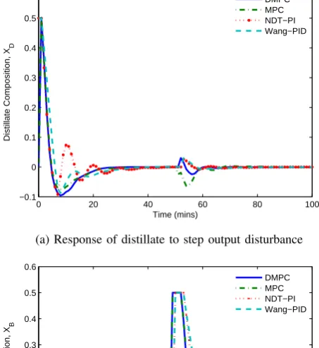
The designed controllers were then implemented to com-pare their set-point tracking and output disturbance rejection. A step reference of 0.5 was applied to the first loop at time
t= 0 and the second loop at timet= 50mins. The results of these are given in Fig. 1. Output step disturbance of 0.5 was also applied to the first and second loops at times
t= 0 andt = 50mins respectively. The resulting plots are also given in Fig. 2. The mean squared error between the set-point and the output obtained with the various controllers are given in Table I.
0 20 40 60 80 100
−0.1 0 0.1 0.2 0.3 0.4 0.5 0.6
Time (mins)
Distillate Composition, X
D
DMPC MPC NDT−PI Wang−PID
(a) Response of distillate to step output disturbance
0 20 40 60 80 100
−0.2 −0.1 0 0.1 0.2 0.3 0.4 0.5 0.6
Time (mins)
Bottoms Composition, X
B
DMPC MPC NDT−PI Wang−PID
(b) Response of bottoms to step output disturbance
[image:4.595.309.536.75.322.2]Fig. 2: Disturbance response
TABLE I: MSE for both set-point tracking and disturbance rejection
Controller Set-point Disturbance rejection XD XB XD×10−3 XB×10−2
MPC 0.2414 0.1087 4.7006 1.3415
DMPC 0.2411 0.1088 4.6867 1.3647
NDT PI 0.2438 0.1170 6.7597 1.3616
NDT-PI 0.2454 0.1131 8.1202 1.5143
For the set-point tracking, the loop interaction for the DMPC and MPC in the first loop is smaller than that of the PID (PI) controllers. In the second loop the interaction is more pronounced in the DMPC and MPC. This is due to the weighting on the second loop which is deliberately made larger. Typically in an industrial setting, the purity of the distillate is more important. However, the MSE of both loops is lower for the DMPC and MPC (Table I). MPC and DMPC have a similar performance.
[image:4.595.316.537.516.577.2](PI) controllers used in this problem. More improvement in performance is expected when process dead times are larger and when constraints are imposed on the process. These conditions will be investigated in subsequent work.
V. CONCLUSION
This paper proposed a DMPC for TITO processes. Shifted input sequence from the previous step is used to cater for loop interactions thereby avoiding iterations. The perfor-mance of the proposed scheme was compared with MPC and PID (PI) by applying to a coupled processes.
REFERENCES
[1] K. J. strm, T. Hgglund et al.,Automatic tuning of PID controllers. Instrument Society of America, 1988.
[2] J. M. Maciejowski,Predictive control : with constraints. Harlow: Pearson Education, 2002.
[3] D. E. Seborg,Process dynamics and control, 3rd ed. Hoboken, N.J: Wiley, 2011.
[4] S. Tavakoli, I. Griffin, and P. J. Fleming, “Tuning of decentralised pi (pid) controllers for tito processes,”Control Engineering Practice, vol. 14, no. 9, pp. 1069 – 1080, 2006.
[5] Q.-G. Wang, B. Zou, T.-H. Lee, and Q. Bi, “Auto-tuning of multivari-able pid controllers from decentralized relay feedback,”Automatica, vol. 33, no. 3, pp. 319 – 330, 1997.
[6] P. Nordfeldt and T. H¨agglund, “Decoupler and PID controller design of TITO systems,”Journal of Process Control, vol. 16, no. 9, pp. 923–936, Oct. 2006.
[7] J. Garrido, F. V´azquez, and F. Morilla, “Centralized multivariable control by simplified decoupling,”Journal of Process Control, vol. 22, no. 6, pp. 1044 – 1062, 2012.
[8] I. Alvarado, D. Limon, D. M. de la PeAa, J. Maestre, M. Ridao, H. Scheu, W. Marquardt, R. Negenborn, B. D. Schutter, F. Valencia, and J. Espinosa, “A comparative analysis of distributed mpc techniques applied to the hd-mpc four-tank benchmark,” Journal of Process Control, vol. 21, no. 5, pp. 800 – 815, 2011.
[9] B. T. Stewart, A. N. Venkat, J. B. Rawlings, S. J. Wright, and G. Pannocchia, “Cooperative distributed model predictive control,”
Systems & Control Letters, vol. 59, no. 8, pp. 460 – 469, 2010. [10] A. Alessio, D. Barcelli, and A. Bemporad, “Decentralized model predictive control of dynamically coupled linear systems,”Journal of Process Control, vol. 21, no. 5, pp. 705 – 714, 2011.
[11] S. Qin and T. A. Badgwell, “A survey of industrial model predictive control technology,”Control Engineering Practice, vol. 11, no. 7, pp. 733 – 764, 2003.
[12] L. Wang, “A tutorial on model predictive control: Using a linear velocity-form model,” Developments in Chemical Engineering and Mineral Processing, vol. 12, no. 5-6, pp. 573–614, 2004.
[13] Q.-G. Wang, B. Huang, and X. Guo, “Auto-tuning of tito decoupling controllers from step tests,”ISA Transactions, vol. 39, no. 4, pp. 407 – 418, 2000.