The Economic and Social Review, Vol. 27, No. 2, January, 1996, pp. 119-136
Estimation of the Parameter i n the Discrete
"Taxi" Problem, With and Without Replacement
A N N L A R G E Y and
J O H N E . SPENCER
The Queen's University of Belfast
Abstract: In the continuous uniform distribution [0,N], the Maximum Likelihood estimator of N
is known to possess high mean square error for large samples. This paper examines this issue in the discrete case, without replacement (extending the work of Tenenbein) and with replacement. Various other estimators including the Minimum Variance Unbiased estimator and Geary's closest estimator are compared in the continuous and two discrete cases. Recommendations are made for choice of estimator in each case, depending on the sample size and on imprecise information on N.
I I N T R O D U C T I O N
G
i v e n a sample o f n observations f r o m a u n i f o r m d i s t r i b u t i o n w i t h u n k n o w n upper l i m i t , N , can we determine the best estimate of N? The discussion of t h i s problem can be traced back a t least as far as t h e w r i t i n g s o f L a p l a c e o n p r o b a b i l i t y (1812-1814). T h e r e he addressed t h e q u e s t i o n o f w h e t h e r i t was possible to estimate N from a r a n d o m d r a w i n g f r o m a n u r n c o n t a i n i n g balls n u m b e r e d 1 u p to N . Since t h e n t h e same issue has been r e f e r r e d t o i n several w r i t i n g s as the "tramcar" (Jeffreys, 1939), Schrodinger (Geary, 1944), "locomotive" (Mosteller, 1965), " t a x i " (Noether, 1971, K o t z a n d Johnson, 1985) "racing car" (Tenenbein, 1971), or "horse r a c i n g " (Rosenberg a n d Deely, 1976) problem. The scenario i n v o k i n g these names is the p r o b l e m faced b y a spectator of e s t i m a t i n g the t o t a l number, N , of t r a m s , t a x i s , etc., i n t h e t o w n / o n t h e race-course f r o m an observation o f n members o f t h e set, k n o w i n g t h a t members i n the population are numbered consecutively 1,...,N.-buttons. However, m u c h w o r k o n e s t i m a t i o n o f t h e upper l i m i t o f t h e u n i f o r m d i s t r i b u t i o n has centred a r o u n d t h e continuous case, w i t h some references to t h e discrete case b e i n g easily a p p r o x i m a t e d b y t h e continuous case i n t h e i n s t a n c e o f l a r g e N (e.g., Rao, 1 9 8 1 , Geary, 1944) a n d often those papers w h i c h d e a l specifically w i t h t h e p r o b l e m i n t h e discrete context are c o n s t r a i n e d t o t h e s i t u a t i o n w h e r e t h e p o p u l a t i o n is sampled w i t h o u t replace m e n t (e.g., Noether, 1 9 7 1 , Tenenbein, 1971, Rosenberg a n d Deely, 1976).
I n t h i s paper we w i l l r e v i e w t h e results from e s t i m a t i o n i n t h e continuous case, b u t t h e m a i n emphasis w i l l be o n devising a n d c o m p a r i n g estimators for N i n t h e discrete case w i t h a n d w i t h o u t replacement. T h i s w i l l e x t e n d t h e results i n Spencer a n d L a r g e y (1993), especially i n the w i t h replacement case. T h r o u g h o u t we consider e s t i m a t i o n u s i n g classical, non-Bayesian techniques, t h o u g h t h e " t a x i " p r o b l e m can be t r e a t e d u s i n g a Bayesian approach. F o r a n e x a m p l e see Rosenberg a n d D e e l y ( i b i d ) , w h e r e B a y e s i a n a n d e m p i r i c a l B a y e s i a n e s t i m a t o r s for t h e zero-one, l i n e a r a n d q u a d r a t i c loss functions are applied t o t h e discrete case w i t h o u t replacement.
I I R E V I E W O F T H E C O N T I N U O U S C A S E
I n the: c o n t e x t o f t h e c o n t i n u o u s u n i f o r m d i s t r i b u t i o n U [ 0 , N ] , w i t h N u n k n o w n , l e t x1 ; x2, —, xn represent t h e observed sample o b t a i n e d f r o m n
i n d e p e n d e n t d r a w i n g s f r o m t h e p o p u l a t i o n , a n d set m a x [ x ! , x2, xn] = w ,
i.e., w r e p r e s e n t s t h e l a r g e s t v a l u e i n t h e sample. P r o p e r t i e s o f t h i s d i s t r i b u t i o n a n d t h e performance o f various estimators o f N are e x a m i n e d i n Spencer a n d L a r g e y (1993). E s t i m a t o r s considered are:
W = m a x i m u m sample value, t h e m a x i m u m l i k e l i h o o d estimator ( M L E ) U = ( n + l ) W / n , t h e u n i q u e m i n i m u m v a r i a n c e u n b i a s e d e s t i m a t o r
( M V U E ) ( D a v i s , 1951; W a s a n , 1970; R o h a t g i , 1976)
J = ( n + 2 ) W / ( n + l ) , t h e m i n i m u m m e a n square e r r o r ( M S E ) e s t i m a t o r (Johnson, 1950)
G = 21 / nW , Geary's e s t i m a t o r , t h e "closest" e s t i m a t o r f o l l o w i n g P i t m a n ' s
d e f i n i t i o n o f closeness (Geary, 1944).
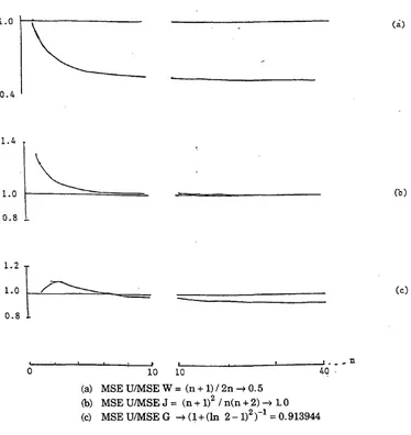
T h e performance of each is assessed t h r o u g h comparison o f M S E = V a r i a n c e + B i a s2, as advocated b y J o h n s o n (1950), a n d r e s u l t s are s u m m a r i s e d i n
Figure 1. •
T h e m o s t s t r i k i n g r e s u l t from t h e analysis is t h e poor performance o f W as a n e s t i m a t o r . M S E o f W is greater t h a n b o t h M S E o f G a n d M S E of U for n > 1. I n t h e l i m i t a s n - > . t » , w h i l e t h e M S E r a t i o s for G a n d U r e l a t i v e to J t e n d to 1.09 a n d 1 respectively, t h a t for W tends to 2.
Figure 1: Relative Mean Square Errors for Selected Pairs of Estimators ofN: Continuous Case
L.O (a)
0.4
1.4
0.8 1
. -> 1 • i , i 1 " 0 10 10 40 •
(a) MSE U/MSE W = (n + 1) / 2n - » 0.5 (b) MSE U/MSE J = (n + 1 )2 / n(n + 2) - » L 0
(c) MSE U/MSE G - > ( l + (ln 2 - 1 )2) "1 = 0.913944
T h e poor performance o f t h e M L E is perhaps n o t s u r p r i s i n g w h e n we realise t h a t t h e l i k e l i h o o d function does not adhere to t h e s t a n d a r d r e g u l a r i t y conditions w h i c h are sufficient to ensure t h e desirable asymptotic properties of M L E s . For example t h e range o f possible values o f xt depends on the upper
I I I D I S C R E T E CASE
T u r n i n g t o t h e case o f t h e discrete u n i f o r m d i s t r i b u t i o n , w e have t w o separate s i t u a t i o n s to consider, i.e., s a m p l i n g w i t h a n d w i t h o u t replacement. Patel (1973) provides a s u m m a r y of these, a n d t h e continuous case, focusing on completeness, sufficiency a n d m i n i m u m variance u n b i a s e d e s t i m a t i o n . ( G u e n t h e r (1978) discusses some techniques for f i n d i n g M V U e s t i m a t o r s w h i c h are usable i n t h e t a x i problem.) T h e M L , M V U , Geary a n d M M S E e s t i m a t o r s w i l l be considered i n each s i t u a t i o n . ( E s t i m a t o r s based o n t h e m e a n a n d m e d i a n are h i g h l y inefficient a n d as a r e s u l t w i l l n o t be con sidered.) To order our findings we proceed by c o m p a r i n g pairs o f estimators for t h e t w o discrete situations. (References t o continuous case results w i l l be made for clarification or where comparisons are of interest.)
N u m e r i c a l r e s u l t s for a l l estimators (i.e., values o f M S E for various N , n ) are presented i n t h e A p p e n d i x to Table 1 ( s a m p l i n g w i t h o u t replacement case) a n d Table 2 ( s a m p l i n g w i t h replacement).
I n both, discrete cases, f(X;N) = 1/N, X = 1, 2 , N where N is t h e u n k n o w n positive integer t o be estimated.
(1) MLE vs MVUE
(a) S a m p l i n g W i t h o u t Replacement T h e j o i n t p d f of X1 ( X 2 , X n is:
f ( X1, X2, . . . , Xn) = l / N ( N - l ) . . . ( N - n + l ) X ^ L 2 , . . . , N
(1) i = L 2 , . . . , n X i ^ X j , a U i ^ j .
L e t W = m a x ( X i , X2, Xn) . T h i s i s c l e a r l y t h e m a x i m u m l i k e l i h o o d
estimator o f N since t h e l i k e l i h o o d function above is a decreasing function of N . I t is also s t r a i g h t f o r w a r d to show (Tenenbein, 1971)
E W = n ( N + 1 ) / ( n + 1 ) (2)
V a r W - n ( N + 1)(N - n ) / ( n + 1 )2 ( n + 2). (3)
I t is k n o w n t h a t W is sufficient for N a n d t h a t t h e d i s t r i b u t i o n o f W is complete (Tenenbein, op. cit.). W is therefore a complete sufficient statistic so i f t h e r e is a f u n c t i o n of W t h a t is unbiased, t h i s function m u s t be t h e u n i q u e best unbiased estimator. T h u s ,
is accordingly the unique m i n i m u m variance unbiased estimator.
T h i s estimator can be i n t e r p r e t e d as the "average gap" e s t i m a t o r (Noether, 1971; R o h a t g i , 1984; Rao, 1981) i.e., W + average gap, where t h e gaps are t h e gaps or spacings b e t w e e n successive o r d e r e d observations (Spencer a n d Largey, op. cit.).
W h i l e U is unbiased, W is o n l y u n b i a s e d for n = N . U has t h e h i g h e r variance, however, w i t h :
For a n y N , <j> exceeds u n i t y for n = l a n d n > N - 2 . I f n = 2 , <|»1 only i f N < 6 . I f n = N - 3 , <|)>1 o n l y i f N < 6 . Tenenbein, op. cit., calculates (j> for v a r i o u s n a n d N=100, 200.
B e l o w w e present graphs for N = 1 0 , 100 a n d 500. (See also Table 1 for n u m e r i c a l values of MSE.)
I t is clear t h a t U completely outperforms W except for v e r y l o w or v e r y h i g h n . T h e r a p i d i t y w i t h w h i c h the g r a p h declines for l o w n should be noted. W i s o f l i t t l e practical value unless n = l .
(b) S a m p l i n g W i t h Replacement T h e j o i n t p d f o f X ^ . - ^ X j , is:
v a r U / v a r W = ( n + 1 )2 / n2
- > ( N + 1 )2/ N2 a s n - > N .
(5)
Relative M S E can be calculated as:
<|> = M S E U / M S E W = ( n + 1)(N + l ) / n ( 2 N - n). (6)
f ( X1, X2, . . . , Xn) = ( l / N )n, X j = 1 , 2 , . . . , N (7)
A g a i n , W = m a x ( X1, X2, . . . , Xn) i s t h e M L E . (8)
The d i s t r i b u t i o n function of W is G ( w ) = ( w / N )n.
Hence t h e p d f of W is:
g ( w ) = ( w / N )n- ( ( w - l ) / N )n, w = l , 2 , . . . , N a n d (9)
E W = N - I jn/ Nn (10)
E W2 = N2-N21( 2 j + l ) f / Nn. ( I D
(These expressions i n v o l v e sums o f powers o f i n t e g e r s w h i c h can be c a l culated by computer or b y l o o k i n g u p tables. They can also be r e w r i t t e n u s i n g B e r n o u l l i n u m b e r s w h i c h i n t u r n c a n be e v a l u a t e d u s i n g t a b l e s e.g., A b r a m o v i t z a n d Stegun, 1965.)
A s before, W is sufficient for N (Wasan, 1970; R o h a t g i , 1976) a n d t h e d i s t r i b u t i o n o f W is complete (Wasan, op. tit.; R o h a t g i , op. cit.). A c c o r d i n g l y , to f i n d the u n i q u e M V U E estimator o f N , we look for t h e f u n c t i o n of W t h a t is unbiased. T h i s is:
(Wasan, op .cit.; Rohatgi, op. tit.; Guenther, op. cit.)
T h e n o t i o n o f a n "average gap" i n t h i s case is n o t s t r a i g h t f o r w a r d a n d t h e M V U E above does n o t seem to have any such i n t e r p r e t a t i o n .
Notice t h a t u n l i k e the case w i t h o u t replacement, n m a y be u n b o u n d e d l y l a r g e a n d V a r W w i l l r e m a i n positive, as n - » ° ° . Notice also t h a t a p p r o x i mations for large N are possible (see Rohatgi (1984)).
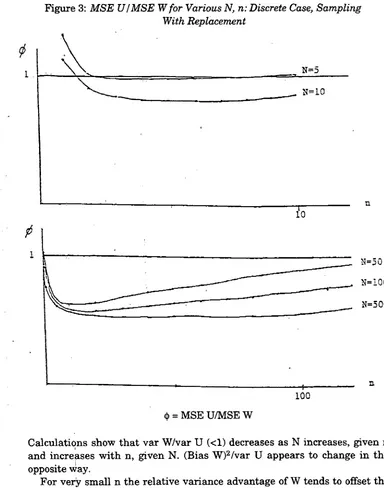
D e f i n i n g <j> = M S E U / M S E W , the results for the w i t h replacement case are s u m m a r i s e d i n F i g u r e 3. (See also Table 2 for n u m e r i c a l results.)
F o r t h e case n = l , w h e r e w i t h a n d w i t h o u t r e p l a c e m e n t coincide, <)> = ( 2 N + 2 ) / ( 2 N - l ) w h i c h is greater t h a n one b u t decreases monotonically t o w a r d s one as N increases.
As n increases, § decreases very sharply at f i r s t , a n d especially r a p i d l y for large N . The graphs show <j>, after the i n i t i a l sharp decline t y p i c a l l y continues to decline slowly (to t h e p o i n t n=3 for N = 5 , to n = 4 for N = 9 , to n = 9 for N = 5 0 , t o n = 1 4 for N = 1 0 0 , t o n=30 for N = 5 0 0 , to n=44 for N = 1 0 0 0 ) a n d t h e n s l o w l y rises u l t i m a t e l y exceeding 1 ( w h e n n = 9 for N = 5 , w h e n n = 5 6 for N = 1 0 ) . A s n oo, E W —> N , a n d v a r W and v a r U v a n i s h , b u t our calculations show <)> w e l l below u n i t y for even q u i t e large relative values o f n . I n no case does <|> fall below 0.5 ( i t s l i m i t i n the continuous case) b u t for large N , i t does get r a t h e r close to i t . Some m i n i m u m <(> values are as follows: N = 1 0 0 , n = 1 5 , <)> = 0.578; N=500, n = 3 1 , <|> = 0.533; N=1000, n=45, <)> = 0.523.)
N o t e t h a t :
(12)
F i g u r e 3: MSE U/MSE Wfor Various N, n: Discrete Case, Sampling With Replacement
N=50
U = i 0 0
N=500
<{> = M S E U / M S E W
C a l c u l a t i o n s show t h a t v a r W / v a r U (<1) decreases as N increases, g i v e n n a n d increases w i t h n , g i v e n N . (Bias W )2/ v a r U appears t o change i n t h e
opposite way.
F o r v e r y s m a l l n t h e r e l a t i v e variance advantage o f W tends t o offset t h e b i a s d i s a d v a n t a g e , so t h a t M L E does r e a s o n a b l y w e l l for v e r y l o w n , especially i f N is n o t too h i g h .
[image:8.479.33.417.67.555.2]t h a t <)> is above 1 for n = l b u t falls below 1 for n = 2 ( N > 7 ) reaches a m i n i m u m q u i c k l y a n d t h e n rises slowly. (For N = 1 0 , <(> reached 1 a t n = 5 6 ; for N = 2 0 , <[» reached 1 a t n=247; a n d for N=50, <|> reached 1 a t n=816.) j
I n t h e continuous case, <j> fell monotonically as n increased, r e a c h i n g 0.5 i n the l i m i t . I n t h e discrete case w i t h o u t replacement, i t is clear, t h a t
and, j u d g i n g from our calculations, t h i s seems t o h o l d i n t h e w i t h replacement case also.
E x a m i n a t i o n o f t h e graphs suggests t h a t t h e w i t h r e p l a c e m e n t case is closer t h a n t h e w i t h o u t replacement case to t h e continuous case, p r i m a r i l y because o f the slowness w i t h w h i c h 0 increases after i t s i n i t i a l drop. A s i m i l a r conclusion holds u s i n g \|/ as the reference — see below.
(2) The Geary Estimator vs MVUE
G is defined to be 21 / nW , a n d i n t h e continuous case ( a n d i n t h e discrete
case w i t h replacement) is t h e "closest" estimator.
I t s b e h a v i o u r r e l a t i v e to t h e M V U E e s t i m a t o r i n t h e t h r e e cases is r a t h e r similar.
I n t h e continuous case, w r i t i n g M S E U / M S E G = \|/(n),
\|/(1) = 1, \|/(2) = 1.0928 a n d \(/ t h e n steadily declines as n rises.
I n fact: \|/(n) < 1 for n > 7
\|/(n) - > .'913944 as n - > °°.
I n t h e discrete cases, w r i t e M S E U ( n , N ) / M S E G ( n , N ) = \|/(n, N ) .
<|> = ( n + l ) ( N + l ) / n ( 2 N - n ) > j , a l l n , N (14)
(a) S a m p l i n g W i t h o u t Replacement
E G = N + l f o r n = l
(15) = 2i , I NN f o r n = N
V a r G = 22 / nn ( N + l ) ( N - n ) / ( n + 2 ) ( n + l )2
(16) = 0 for n = N
M S E G ( n = N ) = N2( l - 21 / N)2
- » ( l o ge 2 )2 a s N - » ° oo (17)
=.480453.
Since M S E U = v a r U = ( N + 1)(N - n ) / ( n + 2 ) ( n + 1 )2, i t is clear t h a t G w i l l
V|/(1,N) = ( N2- 1 ) / ( N2+ 2 ) < 1
(18) 1)7(2, N ) > 1 i f a n d o n l y i f N > 6.
F o r l o w values o f n > 2, i t is clear from t h e graphs ( F i g u r e 4) t h a t G does excellently r e l a t i v e t o U . O n l y w h e n n exceeds about 0.4 N , does t h e g r a p h decline s i g n i f i c a n t l y — t h o u g h after t h a t i t does t e n d to decline r a p i d l y . A t t h a t stage, o f course, M S E U and M S E G are b o t h r a t h e r low.
(b) S a m p l i n g W i t h Replacement For n = l , v a r U = ( N2- l ) / 3
E G = N + 1 (19)
V a r G = ( N2- l ) / 3 (20)
M S E G = ( N2 + 2 ) / 3 (21)
\|/(1,N) = ( N2- 1 ) / ( N2+ 2 ) < 1 . (22)
F r o m the graphs shown i n F i g u r e 5, for n = 2 , > 1. A s n increases, \|/ falls s l o w l y i n i t i a l l y ( r e m a i n i n g above 1 for values o f n q u i t e h i g h r e l a t i v e t o N ) , b u t decreases more r a p i d l y after reaching 1.
G does p a r t i c u l a r l y w e l l for N quite large (say 50 or more) a n d n between 2 a n d about 0 . 9 N . T h e advantage can be q u i t e s u b s t a n t i a l . F o r example, i f N = 5 0 , n=3, M S E U=166.52, M S E G=153.29. The bias i n G is more t h a n offset by a l o w variance.
I V M I N I M U M M E A N S Q U A R E E R R O R
E x a m i n i n g t h e general problem of f i n d i n g t h e m i n i m u m M S E estimator for 9 o f t h e f o r m XQ + k , w i t h k constant, where 0 is a n estimator o f 8 w i t h finite m e a n a n d variance, t h e m i n i m u m M S E X is found from differentiation to be:
A . * = ( 9 - k ) E 9 / E 92. (23)
The corresponding M S E is:
M S E a*9 + k ) = X*2var 8 + (iCE9 + k - 9 )2
F i g p r e 5: MSE U/MSE G for Various N, n: Discrete Case, Sampling With Replacement
f
y = M S E U / M S E G
C l e a r l y t h i s d i m i n i s h e s as k tends towards 0, i.e., as X* - » 0 a n d t h e estimator t e n d s t o w a r d s 9. A s 9 is u n k n o w n t h i s fact i s o f l i t t l e p r a c t i c a l significance, t h o u g h i t is w o r t h n o t i n g t h a t w h e n 9 is a positive integer, as i n t h e discrete t a x i p r o b l e m , a negative k is worse t h a n k = 0. I f k = 0, X* is n o t necessarily dependent o n 9.
I n t h e c o n t i n u o u s t a x i p r o b l e m w i t h k = 0 , 9 = N a n d 9 set t o W , X = N E W / E W2 = ( n + 2 ) / ( n + l ) . T h u s t h e estimator J = ( n + 2 ) W / ( n + l ) has m i n i m u m
( N - k ) ( n + 2 ) W / N ( n + l ) + k . (25)
(a) T h e Discrete Case W i t h o u t Replacement
I n t h e discrete case w i t h o u t replacement, w h e n k = 0 , t h e m i n i m u m M S E estimator of t h e form AW is:
J* = A*W = ( n + 2 ) W / ( n + l + n / N )
(26) = W f o r n = N .
W i t h N u n k n o w n , t h i s is n o t available, t h o u g h i t shows t h a t J = ( n + 2 ) W / (n+1) w i l l have m i n i m u m M S E among estimators of t h e f o r m AW i f n is s m a l l r e l a t i v e t o N . N o t e also t h a t i f n / N is close t o one, M L E w i l l have m i n i m u m M S E among estimators of the f o r m AW.
Since t h e M V U E is o f t h e f o r m A W - 1 , we consider other e s t i m a t o r s o f t h e same form, where A depends on n .
M e a n Square E r r o r of ( A W - 1 ) is A2 v a r W + [ A E W - l - N ]2. F r o m t h e
equation for X* above, the o p t i m a l A. is:
A * = ( n + 2)(N + l ) / ( n + N ( n + l ) ) . (27)
The M i n i m u m M e a n Square E r r o r estimator i n the class AW-1 is t h u s :
L ' ^ ' W - X (28)
= ( n + 2 ) ( l + l / N ) W / ( n + H - n / N ) - l
w h i c h collapses t o
L = ( n + 2 ) W / ( n + l ) - l , f o r s m a l l n / N . (29)
W h e n n = N
L * = ( 1 + 1 / N ) W - L (30)
Since M S E (AW + k ) increases w i t h ( N - k )2, J* m u s t have l o w e r M S E t h a n L * .
Accordingly, from t h e formulae for t h e estimators J a n d L , J m u s t have lower M S E t h a n L p r o v i d e d n / N is sufficiently s m a l l — see Table 1.
Since v a r J a n d v a r L are equal, t h e r e l a t i v e performance of J a n d L t u r n s on t h e r e l a t i v e biases.
Accordingly L w i l l have lower M S E for n large.
I n fact, t h e necessary a n d sufficient c r i t e r i o n is:
L has lower M S E t h a n J i f and only i f 2 N + l < n ( n + 2 ) . (32)
O f course, t h i s c r i t e r i o n involves t h e u n k n o w n N , b u t i t has practical value given vague knowledge o f N . J is better t h a n L for only q u i t e l o w values o f n : n<3, N = 1 0 ; n<13, N=100; n < 4 3 , N=1000.
T h e above t h e o r y and calculations suggest t h a t i f t h e s t a t i s t i c i a n believes J beats L , t h e n J should be used. I t is preferable t o U and w h e n n o t preferable t o G is close t o G — see Table 1. W h e n L beats J , L has v e r y s i m i l a r M S E to t h a t o f U a n d t h e s t a t i s t i c i a n m a y as w e l l choose between U a n d G as d i s cussed i n t h e previous section.
(b) The Discrete Case W i t h Replacement U s i n g t h e a p p r o x i m a t i o n
ln+ 2n+ . . . + ( N - l )n^ Nn + 1/ ( n + l ) , (33)
t o f i n d t h e M M S E estimator of t h e f o r m XW, we have
X* = N E W / E W2^ ( n + 2 ) / ( n + l - ( n + 2 ) / n N )
(34) = ( n + 2) / ( n + 1 ) for N large.
N t E W / E W2) collapses for large N t o J also u s i n g closer approximations.
Accordingly J should do w e l l i f N is large.
T h e c a l c u l a t i o n s , s h o w n i n T a b l e 2, c o n f i r m t h i s , a n d show t h e t h r e e leading estimators as J , G a n d U .
J i n fact does best for s m a l l n , a n y N . For example, J is best for n as h i g h as 3 i f N = 1 0 , as h i g h as 25 i f N = 1 0 0 , a n d as h i g h as 318 i f N=1000. B e y o n d these l i m i t s , e i t h e r G or U emerges as best w i t h t h e i r c o m p a r a t i v e performance as described i n Section I I I .
V C O N C L U S I O N S
T h i s paper has r e v i e w e d a n d f u r t h e r considered e s t i m a t i o n i n t h e t a x i p r o b l e m i n t h e continuous case a n d i n t h e discrete cases w i t h a n d w i t h o u t replacement. T h e estimators discussed were W , t h e m a x i m u m l i k e l i h o o d a n d complete sufficient estimator; U , t h e m i n i m u m variance unbiased e s t i m a t o r (the f o r m u l a for w h i c h depended o n t h e s i t u a t i o n u n d e r c o n s i d e r a t i o n ) ; Geary's e s t i m a t o r G = 21 / nW ; a n d v a r i o u s forms o f M i n i m u m M e a n Square
collapsed t o Johnson's estimator J = ( n + 2 ) W / ( n + l ) . N o t e t h a t a l l estimators are based i n some w a y o n W .
T h e m a x i m u m l i k e l i h o o d e s t i m a t o r W p e r f o r m s p o o r l y i n a l l cases, especially for moderate sample sizes, u s i n g m e a n square e r r o r as t h e k e y c r i t e r i o n . I t s poor a s y m p t o t i c b e h a v i o u r i n t h e c o n t i n u o u s case is n o t r e p l i c a t e d i n t h e discrete cases, however, b u t l a r g e samples are t y p i c a l l y r e q u i r e d for i t to m a t c h t h e M V U e s t i m a t o r i n those cases. T h e odd r e s u l t t h a t t h e M L E estimator does reasonably w e l l for s m a l l samples i n t h e con t i n u o u s case is replicated i n the discrete cases, b u t i t s performance r e l a t i v e to M V U E falls away v e r y r a p i d l y at first as n increases, especially i f N is large.
A r e t h e r e any general recommendations w h i c h can be m a d e as regards choice of a n estimator o f N for t h e various classes o f s i t u a t i o n w e have dealt w i t h ? W e use M S E as t h e k e y c r i t e r i o n , n o t i n g t h a t o t h e r c r i t e r i a (bias, closeness, etc.) could p o i n t i n different directions.
I n the continuous case t h e decision is clear-cut — J should be chosen as i t is t h e M i n i m u m M e a n Square E r r o r estimator i n a w i d e class. I t s advantage is s l i g h t , however, unless n is v e r y l o w (<5). The Geary e s t i m a t o r performs w e l l for s m a l l a n d moderate n , w h i l e for l a r g e r n , U = ( n + l ) W / n i s better t h a n G u n d e r the c r i t e r i o n o f M S E .
I n the discrete case b o t h w i t h a n d w i t h o u t replacement, i t is no longer possible to use t h e exact M M S E estimator since t h i s is now a f u n c t i o n o f t h e u n k n o w n N . The choice o f w h i c h estimator to use is therefore no longer clear. However, t h e f o l l o w i n g tables give a r o u g h idea o f t h e best e s t i m a t o r s , i n t e r m s of m i n i m u m M S E , to use i n v a r i o u s cases. N o t e t h a t t h e e s t i m a t o r L does n o t appear i n t h e w i t h o u t r e p l a c e m e n t t a b l e . L is rejected on t h e grounds t h a t either J , G or U w i l l b e t t e r i t w h e n N is s m a l l , or w h e n n / N is s m a l l , whereas w i t h N large, n / N n o t s m a l l , M S E U approximates M S E L so t h a t l i t t l e is lost by u s i n g U i n t h i s case.
Use of these tables requires e i t h e r some p r i o r i n f o r m a t i o n on N , or t h e a b i l i t y to deduce some i n f o r m a t i o n on N f r o m the observed sample values. I n t h e w i t h o u t replacement case n is m e a s u r e d r e l a t i v e to N , whereas i n t h e w i t h replacement case n is measured i n absolute t e r m s . S denotes s m a l l , M moderate a n d L large.
For t h e special case where n = l t h e ordering of J, W , U , G is clear. F o r t h e continuous case, t h e s i t u a t i o n is,
J W U G E 3N/4 N/2 N N
V a r 3 N2/ 1 6 NP/12 1*73 1*73
M S E 1*74 1*73 r*73 ]SP/3
I n t h e discrete case w h e r e w i t h a n d w i t h o u t replacement coincide w h e n
n = l , .
J W U G E 3 ( N + l ) / 4 ( N + l ) / 2 N N + l V a r 3(N2-1)/16 ( N 2 - D / 1 2 ( N2- ! ) ^ ( N 2 - l ) / 3
M S E ( 2 N2- 3 N + 3 ) / 8 ( 2 N2- 3 N + l ) / 6 ( N 2 - l ) / 3 (N2+2)/3
T h u s M S E J < M S E W i f N > 2 M S E W < M S E U i f N > 1 M S E U < M S E G for a l l N .
REFERENCES
ABRAMOVITZ, M . , and I . STEGUN (eds), 1965. Handbook of Mathematical Func tions, National Bureau of Standards (1964) and New York: Dover Publications, Inc. DAVIS, R.C., 1951. "On M i n i m u m Variance i n Non-regular Estimation", Annals of
Mathematical Statistics, Vol. 22, pp. 43-57.
GEARY, R.C., 1944. "Comparison of the Concepts of Efficiency and Closeness for Consistent Estimates of a Parameter", Biometrika, Vol. 33, No. 2, pp. 123-128. GUENTHER, W.C., 1978. "Some Easily Found M i n i m u m Variance Unbiased Esti
mators", The American Statistician, Vol. 32, No. 1, pp. 29-34. JEFFREYS, H . , 1939. Theory of Probability, Oxford: Clarendon Press.
JOHNSON, N.L., 1950. "On the Comparison of Estimators", Biometrika, Vol. 37, Nos. 3/4, pp. 281-287.
KOTZ, S., and JOHNSON, N.L., 1985. Encyclopedia of Statistical Sciences, Vol. 6, New York: Wiley.
MOSTELLER, F., 1965. Fifty Challenging Problems in Probability, London: Addison-Wesley.
NOETHER, G., 1971. Introduction to Statistics: A Fresh Approach, Boston: Houghton Miflin.
P A T E L , J.K., 1973. "Complete Sufficient Statistics and M V U Estimators", Communications in Statistics, Vol. 2, No. 4, pp. 327-336.
RAO, J.S., 1981. "Estimation Problems for Rectangular Distributions (or the Taxi Problem Revisited)", Metrika, Vol. 28, pp. 257-262.
ROHATGI, V . , 1976. An Introduction to Probability Theory and Mathematical Statistics, New York: Wiley.
ROHATQI, V., 1984. Statistical Inference, New York: Wiley.
SPENCER, J.E., and LARGEY, A., 1993. "Geary on Inference i n Multiple Regression and on Closeness and the Taxi Problem", The Economic and Social Review, Vol. 24, No. 3, pp. 275-295.
T E N E N B E I N , A , 1971. "The Racing Car Problem", The American Statistician, Vol. 25, No. 1, pp. 38-40.
WASAN, M.T., 1970. Parametric Estimation, London: McGraw-Hill. A P P E N D I X
Table 1. MSE of Various Estimators of the Parameters in the "taxi" Problem:
Without Replacement
N=10 U W
1 2 4 6 8 10 34.0000 9.9153 2.7053 1.1887 0.6976 0.5151 33.0000 11.0000 2.7500 0.9167 0.2750 0. 21.6250 8.7407 2.8480 1.4810 1.0151 0.8264 26.1250 10.1852 2.7280 0.9300 0.2867 0.0083 28.5000 12.0000 3.2000 1.0000 0.2667 0. N=100 n 1 4 10 20 50 80 100 3334.0000 380.9633 74.4459 18.0260 2.0809 0.6914 0.4838 3333.0000 404.0000 75.7500 18.3636 1.9423 0.3079 0. 2462.8750 381.5680 74.5304 18.8748 2.8647 1.2773 0.9802 2512.3750 388.6480 75.1998 18.3329 1.9423 0.3081 0. 3283.5000 627.2000 129.5454 31.1688 2.8280 0.3613 0. N=1000
1 333334.000 333333.000 249625.375 250124.875 332833.500
4 39872.737 41541.500 39808.768 39887.848 66267.200
10 8449.272 8258.250 8175.207 8190.752 14925.000
20 2337.600 2229.500 2221.013 2224.552 4200.000
50 • 385.716 365.750 365.847 365.617 698.529
100 91.860 88.323 89.120 88.316 165.987
200 20.034 19.822 20.772 19.821 35.466
500 2.142 1.994 2.986 1.994 2.982
800 0.692 0.312 0.309 0.312 0.374
Table 2: MSE of Various Estimators of the Parameters in the "taxi" Problem: With Replacement
N=10 G U J L W
1 34.0000 33.0000 21.6250 26.1250 28.5000
2 11.0675 12.3138 10.0444 11.9778 13.6500
4 3.7053 4.0379 3.7936 4.4736 4.9677
6 1.8700 1.9723 2.0184 2.3976 2.4288
8 1.1267 1.1482 1.2694 1.5523 1.3829
10 0.7520 . 0.7378 0.8804 1.1344 0.8644
20 0.1985 0.1520 0.2692 0.5974 0.1604
50 0.0023 0.0052 0.0042 0.6602 0.0052
100 0.00486 0.00003 0.00982 0.00003 0.00003
N=100
1 3334.0000 3333.0000 2462.8750 2512.3750 3283.5000
4 395.3097 416.5365 395.5152 403.3232 646.9967
10 83.1911 83.2326 81.9646 83.5448 142.7493
20 22.8285 22.6356 22.6199 23.0607 38.8451
50 3.7356 3.7605 3.9450 4.0869 5.8745
80 1.4367 1.4417 1.6230 1.7748 2.0491
100 0.9098 0.8995 1.0708 1.2462 1.2105
200 0.2149 0.1779 0.2958 0.6106 0.2004
500 0.0241 0.0067 0.0439 0.6580 0.0067
1000 0.00484 4.32E-05 0.01001 0.81030 0.00004
N=1000
1 333334.000 333333.000 249625.375 250124.875 332833.500
4 40020.142 41666.536 39952.320 40032.120 66466.999
10 8542.358 8333.233 8255.677 8272.117 15060.939
20 2392.029 2272.635 2265.396 2269.887 4281.717
50 409.360 384.529 384.251 385.009 734.869
80 161.800 152.354 152.430 152.736 289.095
100 103.713 97.954 98.096 98.299 184.561
500 3.920 3.901 4.109 4.198 6.250
1000 0.931 na 1.093 1.258 1.254