The detection of tethered and rising bubbles using multiple
acoustic techniques
Timothy G. Leighton, David G. Ramble, and Andy D. Phelps
Institute of Sound and Vibration Research, University of Southampton, Highfield, Southampton SO17 1BJ, United Kingdom
~Received 22 January 1996; accepted for publication 10 November 1996!
There exists a range of acoustic techniques for characterizing bubble populations within liquids. Each technique has limitations, and complete characterization of a population requires the sequential or simultaneous use of several, so that the limitations of each find compensation in the others. Here, nine techniques are deployed using one experimental rig, and compared to determine how accurately and rapidly they can characterize given bubble populations. These are, specifically~i!two stationary bubbles attached to a wire; and~ii!injected, rising bubbles. © 1997 Acoustical Society of America.
@S0001-4966~97!00905-3#
PACS numbers: 43.30.Jx, 43.30.Pc, 43.25.Yw, 43.35.Ei@JHM#
INTRODUCTION
Bubble detection is required for many industrial,1 medical,2and environmental3applications.4,5Throughout the range of acoustic techniques by which this can be achieved, there are inherent limitations. If, for example, a signal6,7 is capable of interpretation in terms of assigning homogeneous bulk properties to the ‘‘bubbly liquid’’ as a whole, then such interpretation may be limited to relatively high, relatively spatially uniform, bubble population densities, where the in-terbubble spacing is very much less than the acoustic wave-length. In contrast, other signals may be practicable only at low number densities.8,9Several are prone to false triggering, in that some other object ~e.g., a solid body, or a cluster of small bubbles!10 may give the same signal as that obtained from a given bubble.
In water with ambient pressure p0, an air bubble of radius R0.;10mm has a well-defined resonance frequency
f05v0/2p'0.01(
A
p0)/R0, and pulsates as a lightly damped oscillator: On entrainment the pulsations generate an acoustic ‘‘signature,’’ an exponentially decaying sinusoid, the frequency of which indicates the bubble size.11,12A few milliseconds after entrainment these passive emissions have decayed to below the level of the noise. However, the bubble may still be driven, and active acoustic techniques exploit this acoustic resonance6,7,13,14 through measurements of sound speed, attenuation, scattering, etc. In such procedures, at a particular frequency the acoustic response of a bubbly liquid is taken to be dominated by bubbles which are reso-nant with that frequency. The maximum number of different bubble sizes that can be measured at any one time is deter-mined by the number of different frequencies investigated, which historically is usually one, but in notable cases has been four13 or around nine.7 However, simple linear theory demonstrates that the acoustic scattering cross section of the fundamental frequency is only a local, and not a global, maximum at resonance:15 bubbles very much larger than resonance size can geometrically scatter sound to a greater degree than can smaller, resonant bubbles. If an ultrasonic interrogating signal is employed, the frequency of which is very much higher than the resonances of any bubbles in thesample, geometric scattering can detect bubbles.16–18If MHz sound is, for example, employed to detect mm-sized bubbles, the small wavelengths involved ~'0.4 mm in water at 3.5 MHz!allow the bubble to be located, but do not accurately give the bubble size. Geometric, nonresonant scattering re-lies on the acoustic impedance mismatch between the inho-mogeneity and the surrounding liquid. It is therefore insen-sitive to the nature of the inhomogeneity, and in practice may not distinguish between bubbles and solid bodies of a similar size.
A bubble in an acoustic pressure field P5A cosvpt
tends to linear, low-amplitude oscillations if the driving am-plitude A is small, or if the bubble is far from resonance. However, as the bubble pulsations become larger ~for ex-ample, at resonance!the inherent nonlinearities in the motion become more pronounced, and manifest in the scattered acoustic signal as harmonics of the driving frequency. For example, a quadratic nonlinearity ~i.e., a system response
}P2! will generate harmonics at 2vp; higher-order
nonlin-earities give commensurate harmonics. This has been used to detect bubbles of specific size, resonant at 0.89 MHz in one experiment19and at both this and at 1.64 MHz in another.20 If such systems are to be perfect bubble detectors then the condition must hold that only resonant bubbles can generate the required nonlinearity, and in the presence of only non-resonant bubbles, vp alone is detected. However, while the
emission of the second harmonic is a global maximum at resonance, the 2vp signal can arise through nonbubble
sources of nonlinearity, such as signal distortion in the equipment, which must be carefully examined. Such sources do not include solid inhomogeneities. The same condition holds if the applied field contains two frequencies, i.e.,
P5A cosvpt1B cosvit where vp!vi. The ‘‘imaging’’
frequency (vi) scatters geometrically from a target~the
pul-sating bubble! whose cross-sectional area varies periodically.9The detected signal consists ofvi, modulated
at frequency vp, and the resulting detection of vi6vp in
the received spectrum has been used to size a bubble spec-trum by employing the assumption that, bar the presence of resonant bubbles, only vi and vp are detected.
8,21
as-sumption fails if the pulsation of nonresonant bubbles, or the presence of a quadratic nonlinearity anywhere in the system
~for example, through turbulent water motion!, is sufficient to generate an vi6vp signal. One advantage of
combination-frequency methods is that the bubble resonance generates a signal in the MHz range~close tovi!, removing
it from ‘‘masking’’ signals such as the acoustic input and ambient noise.
All the above techniques for bubble sizing which exploit the bubble resonance suffer in that sources other than reso-nant bubbles~e.g., turbulence, transducer effects, etc.!can to a greater or lesser extent generate the desired signal, indicat-ing the presence of a resonant bubble when one is not present.4Such ‘‘false triggering’’ has not to date been found when signals atvi6vp/2 are used for bubble sizing.9These
signals are generated when the amplitude component A of the insonating field P5A cosvpt1B cosvit exceeds the
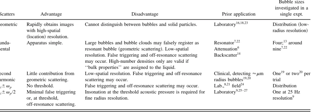
threshold value required to generate Faraday waves on the bubble surface. Characteristics of the various acoustic sizing techniques are summarized in Table I.
The less prone a system is to ‘‘false triggering,’’ the more complicated in general it is to deploy. It therefore would be desirable to be able to deploy a range of these techniques to interrogate a given liquid sample, either se-quentially or concurrently as defined by the problem. This would enable optimization of the process of characterizing the bubble population in the liquid with respect to minimiz-ing the ambiguity of the result and the complexity of the task. The task itself involves first the detection of inhomoge-neities in liquids. In certain circumstances it is then neces-sary to analyze the sample further to distinguish gas bubbles from solid or immiscible liquid-phase inclusions. The final stage of analysis would involve not only the detection, but also the sizing of the gas inclusions, leading to the charac-terization of the bubble population. This can be summarized in a four-part ideal objective:28~i!Detect inhomogeneities in liquids; ~ii! Distinguish gas bubbles from solids; ~iii! Mea-sure radii of bubbles present; ~iv! Measure number of bubbles in each radius class.
This study introduces a method by which the ideal
ob-jective might eventually be achieved, using a range of
tech-niques. The limitations of each can be compensated through the deployment of others. Since the ambiguities of each have been studied theoretically and experimentally,15 the initial emphasis of this study will be how successfully each tech-nique can provide information about simple controlled popu-lations ~stationary single and paired bubbles!. A rising bubble stream will then be measured. The techniques listed in Table I are used, so that bubble detection is achieved through the geometric scattering of 3.5-MHz ultrasound~ us-ing a scanner in both B and M modes simultaneously!, and through scattering of signals at vp, 2vp, vp/2, vi6vp, vi62vp, vi6vp/2, and vi63vp/2. This is done for
broadband, and increasing, incremented, tonal ‘‘pump’’ sig-nals. The study was carried out using relatively low-amplitude acoustic fields to drive the bubble, which is desir-able to minimize the invasiveness of the technique.
I. METHOD
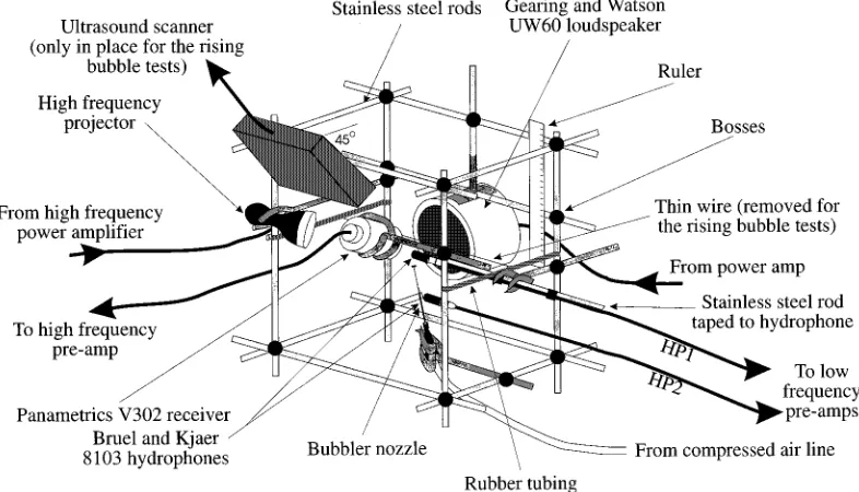
There exist detection zones, at 15-cm depth, for the vari-ous active acvari-oustic sizing systems ~including those listed in Table I!, comprising the overlap of beam patterns of relevant transducers held in rigid ‘‘cage’’ configuration ~Fig. 1!. The cage is placed at depth 0.15 m in a 1.831.231.2-m deep vibration isolated glass-reinforced plastic tank. The bubble population is either injected into the tank below these zones, and then rises to pass through them; or consists of bubbles attached to a wire, held within the intersection of the zones. A Gearing and Watson UW60 loudspeaker ~having a fre-quency response flat to within 65 dB over the range 500 Hz–10 kHz!is used to generate the required ‘‘pump’’ signal. This signal drives the bubbles into oscillation, and it may be broadband, or a series of tones P5A cosvpt, where vp is incremented in 50 Hz~tethered bubbles!or 100 Hz~moving bubbles!steps.
During combination-frequency tests the imaging signal
P5B cosvit is generated by a Therasonic 1030 ~
Electro-Medical Supplies!fixed at 1.134 MHz. A Panametrics V302 receiver detects the MHz signal before it is heterodyned with the Therasonic signal. The Bruel & Kjaer 8103 hydrophone
[image:2.612.57.562.53.235.2]~‘‘HP1’’!is used to detect signals not involving combination
TABLE I. The various acoustic techniques available for bubble detection. Numerals in columns 4 and 5 are references.
Scatters Advantage Disadvantage Prior application
Bubble sizes investigated in a
single expt. Geometric Rapidly obtains images
with high-spatial
~location!resolution.
Cannot distinguish between bubbles and solid particles. Laboratory16,18,23 Distribution~
low-radius resolution!
Funda-mental
Apparatus simple. Large bubbles and bubble clouds may falsely register as resonant bubble~geometric scattering!. Low-spatial resolution. False triggering and off-resonance scattering may occur. High-number densities only are valid if ‘‘bulk properties’’ are assigned to the liquid.
Resonator7,22
Attenuation6
Backscatter14
Four;13around
nine7,22
Second harmonic
Little contribution from geometric scattering.
Low-spatial resolution. False triggering and off-resonance scattering may occur.
Clinical, detecting'mm radius bubbles19,20
One19or two20per
trial
vi6vp No threshold. False triggering and off-resonance scattering may occur. Lab.,8,21field24 Distribution vi6vp/2 Minimal false triggering
or, at threshold,
Insonation at the threshold acoustic pressure is required for fine radius resolution.
Laboratory9,25–27 One at 25 Hz
resolution9
frequencies. The heterodyned high-frequency signal and the B&K 8103 signals are acquired to the PC via a general pur-pose interface bus ~GPIB!-controlled Digital Storage Oscil-loscope ~LeCroy 9314L!. Calibration is made with no bubbles present to allow compensation for the acoustic re-sponse of the water, apparatus, and tank. This enables the sample to be insonated at equal amplitudes when interro-gated by a sequence of tonal pumping signals, each of 0.2-s duration. Data is only collected after a ‘‘start-up’’ time of the first 7.5 ms for tethered bubbles, to allow transients to die away. No such delay can be afforded with rapidly rising mm-sized bubbles, though averaging over the 104samples of each increment reduces the transient effect. Including data collection, the individual incremented tones start 1.6-s apart. The rising bubbles are injected from a needle attached to a compressed air line. The passive acoustic signal so gener-ated is detected by ‘‘HP2,’’ a hydrophone ~Bruel & Kjaer 8103!placed 10 mm from the needle tip at a depth of 29 cm. This signal is analyzed for the exponentially decaying sinu-soid ‘‘signatures’’ which indicate the generation of each bubble, the frequency of the sinusoid revealing the bubble size. However, with higher entrainment rates ~where signa-tures overlap! in noisy environments, individual entrain-ments may not be detected even in time-frequency represen-tation ~TFR!, where resolution in time and frequency is a compromise determined by the size of the window imposed upon the data. However, a TFR of the Gabor coefficients, rather than the acoustic power invested in each frequency band, will readily identify the bubble signatures.29–31A rou-tine uses thresholds on the value and gradient of the Gabor coefficients, then automatically counts and sizes the bubbles, giving their rate of production before they rise into the active detection zones. A second count is made by placing a greased Petri dish in the rising bubble stream above the de-tection zones. Photographic measurement of the bubbles ad-hering to the thin layer of silicone grease were taken.
How-ever, compensation must be made in comparing the bubble population measured in given volumes of liquid by the active techniques, with the captured population on the dish and the rate of bubble generation measured at the needle by the Ga-bor technique. This is because, for example, the volume of the bubble stream sampled by the Petri dish increases with the bubble rise speed. The volume changes caused by the varying hydrostatic pressure are accounted for in comparing all measurements. The sizes of the two bubbles attached to the wire were checked by detaching them from the wire into small glass flasks, in which they were transferred to a trav-eling microscope for measurement.25 A Hitachi EUB-26E 3.5-MHz ultrasound scanner, mounted in the cage, gave M-and B-mode images of the rising bubbles. Atmospheric pres-sure was 0.1003 MPa.
Detection through scattering at vp andvi6vprequires
only linear bubble pulsations, so that the relatively low-energy densities per frequency band afforded by broadband insonation~bandlimited white noise between 1000–8000 Hz! is appropriate. This rapidly allows an estimate of the region wherein the bubble resonances lie, for later application of the nonlinear detection signals (2vp, vp/2, vi6vp/2, vi
62vp,vi63vp/2). These nonlinear signals require an
cremented pure-tone pump signal, rather than broadband in-sonation, for two reasons. First, it is necessary to drive at a sufficiently high amplitude to generate detectable nonlineari-ties. Second, the detector frequency emitted by a bubble dif-fers from that which drives it at resonance, which would cause ambiguity if broadband excitation were employed.
II. RESULTS
A. Two tethered bubbles
[image:3.612.109.502.38.263.2]The first of the results are shown in Fig. 2 for the broad-band excitation of two bubbles attached to a wire 10-mm apart. Throughout the paper a dashed line indicates signal
with no bubbles present; a solid line with crosses indicates the signal in presence of bubble~s!; and a thick solid line with closed circles indicates the ratio of the signal ‘‘with’’ bubbles to that ‘‘without’’ bubbles, i.e., the bubble-mediated amplification. Data points occur at symbols, and at equiva-lent frequencies for dashed lines. Figure 2~a!illustrates the difference in the modulus of the voltage transfer function
~the ratio of output to input!when the bubbles were driven by bandlimited~1–8 kHz! white noise. The response shows peaks at 3.1 and 3.9 kHz (60.1 kHz), with a sharp dip
;300 Hz above each. This reflects the through-resonance behavior of each bubble: At frequencies just below reso-nance the sound field and the bubble pulsations~which scat-ter significantly more than they do away from resonance!are in phase and constructively interfere. However, above reso-nance the bubble undergoes apphase shift such that it now pulsates in antiphase with the driving sound field, resulting in destructive interference. This behavior suggests that the change in signal which results from bubble presence does not represent geometric scattering from a large bubble or other body, but is due to the presence of resonant bubbles in that frequency range. Even several kHz above the resonance of the pair, the detected signal is;1 dB less than the levels at low frequencies, and those found in the absence of bubbles. This is a result of the destructive interference caused by the whole population, and it may be that this can be used to characterize a population @compare this reduction with the smaller one seen in Fig. 2~c!for one of these bubbles on its own#. The coherence between the signal input to the source and the returned signal @Fig. 2~b!#shows a definite bubble-mediated reduction in the signal around 3.360.15 and 4 60.15 kHz. As these coherence dips appear at frequencies midway between the peaks and troughs in the transfer func-tion@Fig. 2~a!#they appear to indicate a bubble nonlinearity rather than a reduced signal to noise ratio, which would be the case if the dips in Fig. 2~a!and~b!occurred at the same frequency.
Figure 2~c! and ~d! show the transfer function and
co-herence resulting from broadband excitation when the bubble resonant at ;3.3 kHz is removed after completion of the two-bubble tests. Its peak disappears @Fig. 2~c!#. The other peak remains at 3.960.1 kHz, suggesting that to within this resolution the bubbles were far enough apart~approximately 10 bubble radii! for the bigger bubble not to significantly influence the resonance frequency of the other.32The peak is about 3 dB higher than in the two bubble test even though the same excitation amplitude was used. This is due to the removal of the antiphase bubble pulsation of the larger bubble beyond its resonance, which therefore means that there is no destructively interfering component on the smaller bubble’s pulsation below its resonance. The coher-ence again shows a similar dip to the relevant one found in the two bubble test @Fig. 2~d!#.
Having, through 1 s ~5 averages! of broadband in-sonation of the two bubbles, reduced the range of interest for further investigation from 1–8 kHz to 2.7–4.7 kHz, the bubble pair was excited~with pump amplitude 120 Pa!at 40 discrete increasing frequencies in 50-Hz increments: At 1.6 s per increment, the test took 64 s. The results are given in Fig. 3 for the harmonic @parts ~a!–~c!# and sum-and-difference
@parts~d!–~f!#signals, monitored simultaneously. The data is displayed as the magnitude in the frequency domain at the location of the signal of interest ~i.e., at vp, 2vp, vp/2,
vi6vp, vi62vp, and vi6vp/2! corresponding to each
pump frequency. The data was sampled at 50 kHz, and the FFT frequency resolution with 8192 points was 6 Hz. The test was repeated following the removal of the larger bubble
~Fig. 4!.
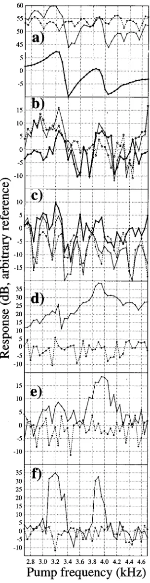
The fundamental backscatter@Fig. 3~a!#shows a rippled amplitude response in the absence of a bubble, which is due to the differences in the proximity of each pumping signal tone to an FFT bin center frequency. This effect disappears when the dB difference~‘‘amplification’’!between the signal with, and without, bubbles is taken, revealing again the char-acteristic through-resonance response indicating the presence of resonant bubbles at 3325670 and 39006100 Hz. The response of the second harmonic@Fig. 3~b!#is less clear. The height of the signal in the absence of the bubble can be affected for instance by the relative levels of harmonic dis-tortion in the equipment and also the proximity of the signal to a frequency bin. Nevertheless, there still appears to be a clear increase in the signal between 3200–3400 and 3800– 4100 Hz. Removal of the larger bubble has negligible effect in the peaks in the first harmonic and second harmonic re-sponse for the smaller bubble as shown in Fig. 4~a!and~b!. The emissions ofvp/2 from both two bubbles@Fig. 3~c!#and
the smaller one@Fig. 4~c!#are too small to differentiate from the noise floor. The amplitude of the heterodyned returned signal from the high-frequency receiver at vi6vp, vi 62vp, andvi6vp/2 are shown in Fig. 3~d!–~f!as a func-tion of the incrementing pumping frequency vp. Though there are maxima at 3.2560.05 and 3.960.2 kHz, the signal atvi6vp@Fig. 3~d!#is present at more than 12 dB above the
‘‘no bubble’’ signal over the entire pumping frequency range. Clearly, the off-resonance contribution to the returned signal limits the resolution of the measurement for the bub-ble’s resonance frequency. Though the off-resonance
contri-FIG. 2. Response@modulus of voltage transfer function, plots~a!and~c!# and coherence @~b!and ~d!#for broadband insonation ~band limited 1–8 kHz!of both@~a!and~b!#tethered bubbles, and for just the smaller@~c!and
bution is less for vi62vp @Fig. 3~e!# the resolution of the
high-frequency peak is similarly poor (460.2 kHz), and there are spurious maxima. It is clear that thevi6vp/2@Fig.
3~f!#signal best shows the presence of two bubbles,
resonat-ing at 3.260.1 and 3.8860.05 kHz. The off-resonance con-tributions are negligible. Removal of the larger bubble dem-onstrates the same features in the detection of the remaining bubble ~Fig. 4! by the ~d! vi6vp, ~e! vi62vp, and ~f!
[image:5.612.98.250.36.626.2]vi6vp/2 signals.
FIG. 3. The HP1 signals for the two-bubble tests~50-Hz increments! show-ing~a!vp, ~b!2vp,~c!vp/2, ~d!vi6vp,~e!vi62vp, ~f!vi6vp/2.
[image:5.612.362.514.37.623.2]Key as for Fig. 2, with open circles showing data points on dashed line.
B. Rising bubbles
Figure 5 shows a portion of the bubble stream as mea-sured through the passive acoustic emissions generated on injection. In Fig. 5~a! a 0.25-s section of the time series recorded by the hydrophone HP2 indicates individual bubbles being repeatably generated every;0.06 s. Each of the bubble signatures has the form, not of a single exponen-tially decaying transient, but of multiple ones, revealing that the released bubble is excited on three subsequent occasions following the initial release from the needle @Fig. 5~b!#. These excitations arise through contact, and usually coales-cence, between the newly released bubble and the successor gas pocket growing at the nozzle tip.33As a result, the plot of the Gabor coefficients@Fig. 5~c!#may reveal multiple peaks for a single bubble ~which vary each time, showing the nozzle process is not entirely repeatable!. Clearly the fre-quency at which the final peak of each group occurs @ ar-rowed in Fig. 5~c!#is the one which relates to the size of the final bubble after it has escaped clear of the contact/ coalescent processes that occur at the nozzle. It is this size which is taken to be a measure of the bubble size upon in-jection.
In Fig. 6 the results of broadband insonation in the fre-quency range 1–8 kHz is shown. In Fig. 6~a!, the signal picked up by HP1 is shown, both for the situation before the bubble stream began, and for the scattered signal in the pres-ence of the bubble stream. The differpres-ence between the two signals is plotted, showing significant changes in the fre-quency range 3.5–5 kHz, indicating the through-resonance effect described above, centered around 460.1 kHz. In Fig. 6~b!, the heterodyned signal from the high-frequency re-ceiver transducer shows bubble-mediated change from 3.5 to 4.9 kHz ~centered at 4.260.3 kHz). An 800-Hz high-pass filter was placed after the heterodyning so that the strong Doppler components of the returned signal did not overload the input channel to the oscilloscope.
Having rapidly found the region of interest ~3.3–4.3 kHz!through the broadband technique, the pump sound field is incremented in this range in steps of 100 Hz, at a pressure amplitude of 240 Pa ~0-pk!. Figure 7 shows the results of analysis of the signal recorded by hydrophone HP1. In Fig. 7~a!, the scattering of the fundamental frequencyvp gives f0'3850620 Hz. The second harmonic 2vp neither
imme-diately indicates a distribution around a single bubble size
[image:6.612.65.284.34.233.2]@Fig. 7~b!#, nor accurately indicates what the size might be ( f0'3.960.2 kHz). The vp/2 results are similarly unclear @Fig. 7~c!#. During the same single pass from 3.2 to 4.4 kHz as was made for Fig. 7, were taken the results for Fig. 8, a histogram showing the received, heterodyned spectrum as a function of the pump frequency~this, on the horizontal axis,
FIG. 5. The HP2 signal during injection.~a!Time series@detail shown in
~b!#. ~c! Time-frequency representation of Gabor coefficients associated with ~a! ~first peak removed for clarity!. Where multiple coefficients are identified with injection of a single bubble, the later one~arrowed!gives natural frequency.
FIG. 6. Response ~modulus of voltage transfer!for broadband insonation
[image:6.612.329.548.40.144.2]~bandlimited 1–8 kHz!of rising bubbles, from~a!HP1, and~b!heterodyned high-frequency~from V302!signals. Resolution: 98 Hz. Key as for Fig. 2.
FIG. 7. Response at ~a!vp, ~b! 2vp, ~c! vp/2 in the HP1 signal for
[image:6.612.354.520.384.709.2]indicating not a continuum but the 12 settings of the pump frequency, since the latter was incremented in 100-Hz steps!. The clearest indication of resonance is that only for the pump frequency setting of 3.7 kHz does structure in the het-erodyned spectrum at frequencies which are multiples of vp/2~corresponding to vp/2, vp, 3vp/2, and 2vp! occur.
All other peaks do not correspond to multiples ofvp. Figure
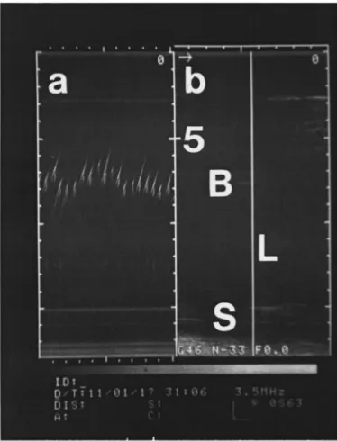
9 shows both the ~a! M- and ~b! B-mode images obtained using the Hitachi ultrasound scanner, the section shown be-ing a slice at 45° to vertical~Fig. 1!. The bubble~labeled B! can be located in Fig. 9~b! ~near field is at top of image!, which also images the loudspeaker ~S!and part of the cage. The images which intersect the vertical line ~L! in 1 s are plotted in Fig. 9~a!: Almost 19 bubbles pass through the beam in that time, with rise speed ~from the image, within the limits of the rectilinear bubble motion, adjusting for the
45° orientation! of 2062 cm/s. Comparison of ‘‘a’’ with ‘‘b’’ allows the transient features~e.g., bubbles!to be distin-guished from the time-invariant ones ~e.g., cage and speaker!.
III. DISCUSSION
For the two tethered bubbles, optical measurements gave radius estimates of 1.160.1 and 0.860.1 mm. Figure 3~f!, which plotsvi6vp/2, most clearly indicates the presence of
two bubbles. Table II summarizes the information gleaned from each signal type in the two-bubble test. Though no high-resolution technique determines both resonances to the same accuracy, the best overall resolution is obtained from vi6vp/2 using incremented pump signals. Initial use of
broadband first reduced the test time by a factor of 64. The resolution of vi6vp/2 can be dramatically affected by the
acoustic pressure at the bubble: While it could be improved to612 Hz by insonating at the threshold pressure,9 there is no guarantee that in the general case this threshold can be accurately delivered.
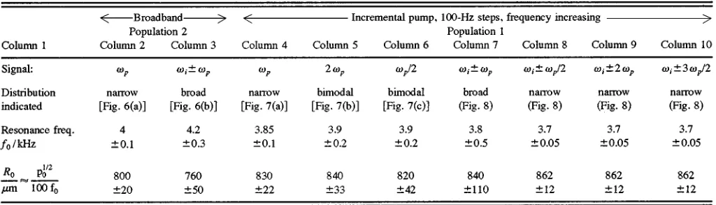
This is particularly true when considering the results from moving bubbles ~Table III!, since each bubble is tran-sitory. Also because of this, not only the accuracy but also the population sampling must be considered. In fact, the re-sults in Table III refer to two quite separate populations. First the incremented techniques ~while they can be repeated to average a steady-state population!9were here in fact applied in one pass, and so would ideally detect signals only from resonant bubbles which are in the detection zone during the 0.2 s of each tone. Since bubbles are generated at ;60 ms intervals, and have a rise time of 2062 cm/s, all the incre-mented tests ~columns 4–10!sample in each increment the same population of ;4 bubbles ~different sets of ;4 bubbles for each of the 40 increments—‘‘population 1’’!. Three minutes later the broadband techniques sample across the entire frequency range for five 0.2-s averages, totalling 1 s: The results in columns 2 and 3 therefore sample a popu-lation of ;19 bubbles ~‘‘population 2’’!. Though there are differences in resolution between the broadband and the in-cremented techniques, the results in Table III indicate that the two populations differed, the one measured first having a lower resonance ~3.760.05 kHz! than the other ~4.060.1 kHz!. This issue will be discussed later.
Resolution of thevpandvi6vpsignals is roughly
con-stant between broadband and incremented forcing at around 100 and 300–500 Hz, respectively~Table III!. Thevpsignal is not pronounced and would readily be confused by a wide range of sizes~see Table II!. The resonance is indicated not by the maximum ~strong emission almost in phase with driver!, but by the in-phase point between the maximum and the minimum ~antiphase! point: This has implications for studies where the scattering is assumed to be from resonant bubbles only. Only the simultaneous occurrence of the struc-ture at vi6vp/2, vi63vp/2, andvi62vp allows accurate
active characterization. It is not surprising that the vi
[image:7.612.83.262.38.174.2]6vp/2 signal should so clearly indicate the resonance,
FIG. 8. Greyscale histogram showing heterodyned received signal ~from V302!for each discrete setting of the pump frequency~100-Hz increments!. Light shades indicate strong signal. Signals at vi6vp/2, vi6vp, vi 63vp/2, andvi62vpare indicated.
[image:7.612.81.268.448.693.2]whereas thevp/2 signal does not, since the surface activity that generates the subharmonic emission cannot itself propa-gate to distance as it does not involve any bubble volume changes. However, as these Faraday waves change the effec-tive area presented to the imaging beam, they can cause a modulation in the scattered signal, and this signal will propa-gate to distance.
The question of whether the two populations, measured by broadband and incremented techniques, could possess the distribution difference suggested above must be addressed by reference to the other techniques used for determining the bubble size some minutes after the conclusion of the broad-band tests. The62-cm/s standard deviation on the 20-cm/s rise time translates34to estimated lower and upper limits for radius in this water of 0.87 and 1.13 mm. Clearly this is not sufficiently discerning. The distribution of rising bubbles from four Petri dish photographs~taken 10 minutes after the end of the passive Gabor tests and corrected for hydrostatic head! gives for the size at 15-cm depth: 790660mm ~28 bubbles collected in 1.5 s!; 7906120mm~24 bubbles in 1.3 s!; 830680mm ~27 bubbles in 1.4 s!; 8206130mm ~32 bubbles in 1.7 s!. There is some indication of occasional larger bubbles in a more uniform distribution.
The actual stability of the population is best determined by the Gabor tests. Three of these were performed at one-minute intervals after the broadband tests, and before the ultrasonic images were taken. In each test 0.25 s of passive emissions, comprising the injection emissions of five con-secutive bubbles, were taken@Fig. 5~a!represents test 2#. The natural frequencies so found are shown in Table IV, with the average for each test, and the calculated bubble size
distri-bution at the needle ~29-cm depth! and at the zone of the active detector ~15-cm depth!. Clearly, variation in the size of the generated bubbles can occur. This is not unexpected when compressed air, supplied from a line, is bubbled at rates high enough for interbubble contact/coalescence to oc-cur. Table IV suggests that the variation found during the 1 s of the broadband test, and the 4031.6 s of the incremented test, is of the same order as the standard deviations quoted in Table III. Clearly for all but the technique with the highest resolution in each population, the standard deviation must represents the resolution limitations of the techniques. For the highest resolution ~columns 8–10 for population 1; col-umn 2 for population 2! the uncertainties in Table III are similar to those quoted for these techniques during the two-bubble test~Table II!, when the population was stable. This suggests that, here too, the standard deviations reflect limits in resolution. It seems that in fact the best resolution limits in each case are very similar to the variability one might expect in the population. Though by no way conclusive, it is sug-gestive that the large standard deviations in tests 1 and 3 result from single outlying values. These values could well escape detection in the 0.2-s duration of each incremented tone, and if the item 3190 Hz is removed from test 1 the average becomes 3686690 Hz~871621 and 875621mm at 29- and 15-cm depth, respectively!, and if the item 3219 Hz is eliminated from test 3, the average becomes 4004630 Hz
~giving 80266 and 80666 mm at 29- and 15-cm depth, re-spectively!. This variation is less than the resolution limits of Table II and the uncertainties quoted in Table III, for the vi6vp/2 and related tests.
The Gabor technique for sizing bubbles from their
[image:8.612.53.567.52.169.2]pas-TABLE II. Resonances and calculated radii of the two tethered bubbles ( p05101 770 Pa!. References in row 2 are to figures.
[image:8.612.53.565.595.742.2]sive ringing upon formation is not only the most simple and accurate but also samples the entire population, being ca-pable of logging the natural frequency of each and every bubble that is generated in near real time to 1 Hz accuracy
~even giving details of nozzle processes!. However, the Ga-bor signal must be interpreted carefully. It reflects the natural frequency of a damped system, given byv0(12d2), where d is the dimensionless damping coefficient35 andv0 the un-damped natural frequency: Active techniques in general measure the maximum of the amplitude response, which oc-curs at frequencyv0(122d2). The two major limitations of the Gabor technique are, first, that the signal becomes creasingly difficult to interpret as the entrainment rate in-creases. Second, passive emissions usually give information only about the bubbles being entrained during the measure-ment interval, the excitation that is strong enough to make adequate emissions usually requiring the closure of a liquid surface:15Older, ‘‘silent’’ bubbles would have to be excited by impulse to ring, and a sufficiently strong impulse would alter the bubble population by inducing more closures ~i.e., fragmentation!.
IV. CONCLUSIONS
Broadband insonation rapidly indicates the range over which bubble resonances may occur, reducing the time re-quired for tonal incrementation. Best resolution and popula-tion sampling was achieved using the Gabor technique, though this operates only on entrainment. The best active indicator of the bubble population in these tests, where a relatively low-amplitude pump signal was employed to mini-mize the invasiveness of the technique,36 was thevi6vp/2
signal. However, it must be remembered that this signal is not simple to implement: For best resolution the acoustic pressure amplitude at the bubble must be close to the threshold,9and a delay~after insonation at a given frequency commences!is recommended, to allow the transients to de-cay before data is acquired.
ACKNOWLEDGMENTS
Our thanks to EPSRC~Reference No. GR/H 79815!and NERC ~GR3/9992! for funding, and to P. R. White for ad-vice.
1R. M. Detsch and R. N. Sharma, ‘‘The critical angle for gas bubble
en-trainment by plunging liquid jet,’’ Chem. Eng. J. 44, 157–66~1990!.
2E. G. Tickner, ‘‘Precision microbubbles for right side intercardiac
pres-sure and flow meapres-surements,’’ in Contrast Echocardiography, edited by R. S. Meltzer and J. Roeland~Nijhoff, London, 1982!.
3D. K. Woolf, ‘‘Bubbles and the air-sea transfer velocity of gases,’’
Atmos.-Ocean 31, 451–474~1993!.
4
T. G. Leighton, ‘‘Acoustic Bubble Detection. I. The detection of stable gas bodies,’’ Environ. Eng. 7, 9–16~1994!.
5T. G. Leighton, ‘‘Acoustic Bubble Detection. II. The detection of transient
cavitation,’’ Environ. Eng. 8, 16–25~1995!.
6H. Medwin, ‘‘In situ acoustic measurements of microbubbles at sea,’’ J.
Geophys. Res. 82, 971–976~1977!.
7
H. Medwin and N. D. Breitz, ‘‘Ambient and transient bubble spectral densities in quiescent seas and under spilling breakers,’’ J. Geophys. Res.
94, 12751–12759~1989!.
8
V. L. Newhouse and P. M. Shankar, ‘‘Bubble size measurement using the nonlinear mixing of two frequencies,’’ J. Acoust. Soc. Am. 75, 1473– 1477~1984!.
9
A. D. Phelps and T. G. Leighton, ‘‘High resolution bubble sizing through detection of the subharmonic response with a two frequency excitation technique,’’ J. Acoust. Soc. Am. 99, 1985–1992~1996!.
10
R. Y. Nishi, ‘‘Ultrasonic detection of bubbles with Doppler flow transduc-ers,’’ Ultrasonics 10, 173–179~1972!.
11M. Strasberg, ‘‘Gas bubbles as sources of sound in water,’’ J. Acoust. Soc.
Am. 28, 20–26~1956!.
12T. G. Leighton and A. J. Walton, ‘‘An experimental study of the sound
emitted from gas bubbles in a liquid,’’ Eur. J. Phys. 8, 98–104~1987!.
13D. M. Farmer and S. Vagle, ‘‘Waveguide propagation of ambient sound in
the ocean-surface bubble layer,’’ J. Acoust. Soc. Am. 86, 1897–1908
~1989!.
14S. A. Thorpe, ‘‘Measurements with an Automatically Recording Inverted
Echo Sounder; ARIES and the Bubble Clouds,’’ J. Phys. Oceanogr. 16, 1462–1478~1986!.
15T. G. Leighton, The Acoustic Bubble~Academic, London, 1994!, pp. 234–
243, 295–298, 439–464.
16S. L. Morriss and A. D. Hill, ‘‘Ultrasonic imaging and velocimetry in
two-phase pipe flow,’’ Trans. ASME, J. Heat Transf. 115, 108–116
~1993!.
17R. Van Der Welle, ‘‘Void fraction, bubble velocity and bubble size in two
phase flow,’’ Int. J. Multiphase Flow 11, 317–45~1985!.
18W. F. Kolbe, B. T. Turko, and B. Leskovar, ‘‘Fast ultrasonic imaging in a
liquid filled pipe,’’ IEEE Trans. Plasma Sci. 33, 715–722~1986!.
19D. L. Miller, ‘‘Ultrasonic detection of resonant cavitation bubbles in a
flow tube by their second harmonic emissions,’’ Ultrasonics 19, 217–24
~1981!.
20
D. L. Miller, A. R. Williams, and D. R. Gross, ‘‘Characterization of cavi-tation in a flow-through exposure chamber by means of a resonant bubble detector,’’ Ultrasonics 22, 224–230~1984!.
21R. M. Schmitt, H. J. Schmidt, B. Grohs, H. P. Schwarz, and M. Biebinger,
‘‘Bubble sizing in the lower micron range based on the 2-frequency in-sonification method,’’ Ultrason. Imaging 9, 63–64~1987!.
22
N. Breitz and H. Medwin, ‘‘Instrumentation for in-situ acoustical mea-surements of bubble spectra under breaking waves,’’ J. Acoust. Soc. Am.
86, 739–43~1989!.
23J. Wolf, ‘‘Investigation of bubbly flow by ultrasonic tomography,’’ Part.
Part. Syst. Charact. 5, 170–173~1988!.
24D. Koller, Y. Li, P. M. Shankar, and V. L. Newhouse, ‘‘High-speed
bubble sizing using the double frequency technique for oceanographic applications,’’ IEEE J. Oceanic Eng. 17, 288–291~1992!.
25T. G. Leighton, R. J. Lingard, A. J. Walton, and J. E. Field, ‘‘Acoustic
bubble sizing by the combination of subharmonic emissions with an im-aging frequency,’’ Ultrasonics 29, 319–323~1991!.
26A. D. Phelps and T. G. Leighton, ‘‘Investigations into the use of two
frequency excitation to accurately determine bubble sizes,’’ in Bubble
Dynamics and Interface Phenomena, Proceedings of an IUTAM Sympo-sium, edited by J. R. Blake, J. M. Boulton-Stone, and N. H. Thomas
~Kluwer Academic, Dordrecht, The Netherlands, 1994!, pp. 475–483.
27A. D. Phelps and T. G. Leighton, ‘‘Acoustic bubble sizing using two
frequency excitation techniques,’’ Proceedings of the 2nd European
Con-ference on Underwater Acoustics, Copenhagen, 1994, edited by L. Bjorno
~European Commission, Luxenbourg, 1994!, pp. 201–206.
28T. G. Leighton, A. D. Phelps, D. G. Ramble, and D. A. Sharpe,
‘‘Com-TABLE IV. Natural frequencies and calculated average radii from Gabor tests at 29, and 15-cm depths.
Trial Test 1 Test 2 Test 3 Natural frequencies/Hz 3722 3751 4018 3737 3699 4015 3190 3642 3219 3550 3758 3965 3736 3835 4021 Average freq./Hz 3580 3740 3850
6240 670 6350
R0/mm at 29 cm 897 859 834
660 615 676
R0/mm at 15 cm 901 863 838
[image:9.612.52.298.56.193.2]parison of the abilities of eight acoustic techniques to detect and size a single bubble,’’ Ultrasonics 34, 661–667~1996!.
29T. G. Leighton, M. F. Schneider, and P. R. White, ‘‘Study of dimensions
of bubble fragmentation using optical and acoustic techniques,’’
Proceed-ings of the Sea Surface Sound, Lake Arrowhead, California, 1994, edited
by M. J. Buckingham and J. Potter~World Scientific, Singapore, 1995!, pp. 414–428.
30
A. D. Phelps, T. G. Leighton, M. F. Schneider, and P. R. White, ‘‘Acous-tic bubble sizing, using active and passive techniques to compare ambient and entrained populations,’’ ISVR Technical Report No. 229, University of Southampton, UK, 1994.
31A. D. Phelps, T. G. Leighton, M. F. Schneider, and P. R. White, ‘‘Active
and passive acoustic bubble sizing,’’ ISVR Technical Report No. 237, University of Southampton, UK, 1994.
32M. Strasberg, ‘‘The pulsation frequency of nonspherical gas bubbles in
liquids,’’ J. Acoust. Soc. Am. 25, 536–537~1953!.
33T. G. Leighton, K. J. Fagan, and J. E. Field, ‘‘Acoustic and photographic
studies of injected bubbles,’’ Eur. J. Phys. 12, 77–85~1991!.
34
R. Clift, J. R. Grace, and M. E. Weber, Bubbles, Drops and Particles
~Academic, New York, 1978!.
35C. Devin, Jr., ‘‘Survey of Thermal, Radiation, and Viscous Damping of
Pulsating Air Bubbles in Water,’’ J. Acoust. Soc. Am. 31, 1654~1959!.
36T. G. Leighton, A. D. Phelps, and D. G. Ramble, ‘‘Bubble detection using
low amplitude multiple acoustic techniques,’’ Proceedings of the 3rd
Eu-ropean Conference on Underwater Acoustics, Heraklion, 1996, edited by