Statistical Correlation Analysis of Field-Aligned Currents
Measured by Swarm
J. -Y. Yang1,2 , M. W. Dunlop1,3,4 , H. Lühr5, C. Xiong5 , Y.-Y. Yang6 , J. -B. Cao1 ,
J. A. Wild7 , L.-Y. Li1 , Y.-D. Ma1, W.-L. Liu1 , H.-S. Fu1 , H.-Y. Lu1, C. Waters8 , and P. Ritter5
1
Space Science Institute, School of Space and Environment, Beihang University, Beijing, China,2Key Laboratory of Earth and Planetary Physics, Chinese Academy of Sciences, Beijing, China,3RAL_Space, STFC, Chilton, Oxfordshire, UK,4The Blackett
Laboratory, Imperial College London, London, UK,5GFZ, German Research Centre for Geosciences, Potsdam, Germany,6The Institute of Crustal Dynamics, China Earthquake Administration, Beijing, China,7Department of Physics, Lancaster
University, Lancaster, UK,8School of Mathematical and Physical Sciences, University of Newcastle, Callaghan, New South Wales, Australia
Abstract
We investigate the statistical, dual-spacecraft correlations of field-aligned current (FAC) signatures between two Swarm spacecraft. For thefirst time, we infer the orientations of the current sheets of FACs by directly using the maximum correlations obtained from sliding data segments. The current sheet orientations are shown to broadly follow the mean shape of the auroral boundary for the lower latitudes and that these are most well ordered on the dusk side. Orientations at higher latitudes are less well ordered. In addition, the maximum correlation coefficients are explored as a function of magnetic local time and in terms of either the time shift (δt) or the shift in longitude (δlon) between Swarms A and C for variousfiltering levels and choice of auroral region. Wefind that the low-latitude FACs show the strongest correlations for a broad range of magnetic local time centered on dawn and dusk, with a higher correlation coefficient on the dusk side and lower correlations near noon and midnight. The positions of maximum correlation are sensitive to the level of low-passfilter applied to the data, implying temporal influence in the data. This study clearly reflects the two different domains of FACs: small-scale (some tens of kilometers), which are time variable, and large-scale (>50 km), which are rather stationary. The methodology is deliberately chosen to highlight the locations of small-scale influences that are generally variable in both time and space. We may fortuitouslyfind a potential new way to recognize bursts of irregular pulsations (Pi1B) using low-Earth orbit satellites.1. Introduction
The Earth’s field-aligned currents (FACs) are the dominant process by which energy and momentum are transported between the magnetosphere and the ionosphere-thermosphere system (e.g., Foster et al., 1983; Lu et al., 1998; Yu et al., 2010), and therefore, FACs are fundamentally important for the understanding of magnetosphere-ionosphere coupling. The upward FAC is responsible, at least in part, for the heating of the ionospheric electrons, although it is less clear whether the downward FAC cools the ionosphere (Pitout et al., 2015; Wing et al., 2015).
Both large- and small-scale FACs have been observed in the auroral zone extending over several degrees of magnetic latitude. Large-scale FACs (the Birkeland current system), with perturbations on spatial scales larger than 50 km at low-Earth orbit (LEO) satellite altitudes, have been described by Iijima and Potemra (1976a) in terms of“Region 1”(R1) and“Region 2”(R2) systems, which couple the external magnetospheric currents to the high-latitude ionosphere and the inner magnetosphere to the auroral ionosphere. Iijima and Potemra (1978) later found that the FACsflow into R1 on the dawn side and away from R1 (out of the ionosphere) on the dusk side. They also found that the currentflow in R2 is reversed with respect to R1 at any given local time except in the Harang discontinuity region, ~20:00–24:00 magnetic local time (MLT; Harang, 1946) and cusp MLT, where theflow patterns are more complicated. There is evidence that the large-scale FACs are gen-erated by the“long-term”interaction of the solar wind with the magnetosphere (for recent work, see Wing et al., 2015, which showed upward R1 currents can be driven by solar wind velocity shears at the magneto-pause), although these current sheets can often have complicated spatial and temporal variations (heresheet refers to the discussion of the azimuthal extent of R1/R2 FACs in this paper). Small-scale FACs are usually
RESEARCH ARTICLE
10.1029/2018JA025205
Key Points:
• For thefirst time, we infer the orientations of the current sheets of FACs using a maximum correlation method
• This study clearly reflects two different domains of FACs: small-scale, which are time variable, and large-scale, which are rather stationary
• Wefind a potential new way to recognize bursts of irregular pulsations (Pi1B) using low-earth orbit satellites
Correspondence to:
M. W. Dunlop, [email protected]
Citation:
Yang, J. -Y., Dunlop, M. W., Lühr, H., Xiong, C., Yang, Y.-Y., Cao, J. -B., et al. (2018). Statistical correlation analysis of
field-aligned currents measured by Swarm.Journal of Geophysical Research: Space Physics,123. https://doi.org/ 10.1029/2018JA025205
Received 10 JAN 2018 Accepted 18 SEP 2018
Accepted article online 28 SEP 2018
characterized by quasi-equal, parallel sheets of current into and out of the ionosphere with latitudinal thick-nesses of tens of kilometers at LEO altitudes and with typical timescales of order 10 s or less. These small-scale FACs are associated with“short-lived”plasma processes within the magnetosphere such as discrete auroral arcs (Anderson & Vondrak, 1975),field-line resonances (Pitout et al., 2003; Rankin et al., 1999; Waters & Sciffer, 2008), bursty bulkflows in the plasma sheet (Merkin et al., 2013; Yu et al., 2017), and associated Pi2 (Cao et al., 2008, 2010), as well as Pi1 waves, which will be discussed in detail in section 3.3.
Nevertheless, separation of the temporal and spatial nature of both small- and large-scale FACs has been notoriously difficult (e.g., see Lühr et al., 2015; Stasiewicz et al., 2000) since these currents are both highly dynamic and vary in size, while single spacecraft estimates generally require assumptions of either geometry (such as infinite sheets, as adopted by, e.g., Anderson & Vondrak, 1975; Marshall et al., 1991) or some degree of time stationarity (to applydB/dtto a spatial estimate, where multispacecraft estimates are unavailable; Dunlop et al., 1988, for comparison). Despite this problem, since thefirst identification of FACs (Iijima & Potemra, 1976a; Zmuda et al., 1966; Zmuda et al., 1967), many previous, typically statistical, studies have been performed, using single-spacecraft and multispacecraft methods, or indirect observations, to probe their glo-bal natures (e.g., Anderson et al., 2000; Gjerloev et al., 2011; Dunlop et al., 2015). An investigation of the char-acteristics of FACs that are restricted in both their spatial and temporal variations between multiple spacecraft positions has also recently been carried out by Forsyth et al. (2017; through the development of a rigorous test of purely static, 1-D normal current sheets) and has been applied recently in a study by McGranaghan et al. (2017).
The alignment of current sheets of large-scale FACs is generally along the boundary of the auroral oval but can be noticeably distorted during very disturbed periods (Iijima & Potemra, 1978). Nevertheless, it has been argued that the basic pattern may often be maintained (Gjerloev & Hoffman, 2014), although the intensity of currents varies from event to event. Here we have used the recently acquired Swarm multispacecraft data set between April 2014 and April 2016 to investigate the MLT dependence of the correlations between the two spacecraft FAC sheets with a new method using statistical analysis of the interspacecraft maximum correla-tions between FAC signatures, which also shows directly the auroral alignments of the current sheets. The sensitivity of this analysis to thefiltering of the data and both the time delay and longitudinal separation between the spacecraft are explored. The statistical work shows differences between large-scale FAC sheets, which occur mainly in the dawn and dusk sectors and more localized current sheets possibly associated with the NBZ (as defined by Iijima et al., 1984) and cusp currents (Iijima & Potemra, 1976b), also referred to as Region 0 currents (Bythrow et al., 1988).
2. Methodology
The Swarm mission (Friis-Christensen et al., 2008) consists of three spacecraft (A, B, and C)flying in phased, circular, low-Earth polar orbits since launch on 22 November 2013. The data set used here was mainly the FAC signals derived from the Swarms A and C observations during thefinal constellation phase (operations from 17 April 2014), where the two spacecraft had orbital periods of ~94 min,flying side by side at a mean high-latitude altitude of about 470 km, and sampling all local times in about 132 days. The third spacecraft Swarm B flies at a slightly higher orbit at ~531-km altitude, with a slightly different orbital period of ~95 min and drifts in MLT with respect to Swarms A and C, which remain close together throughout the time period studied here. The three Swarm spacecraft move through the auroral regions and across the polar cap as a result of their near polar orbits.
We use the official 1-Hz Level-2 OPER (Routine Operations offile class) FAC data taken from the vectorfl ux-gate magnetometer (Friis-Christensen et al., 2008; Ritter et al., 2013; Stolle et al., 2013) on Swarm. To minimize the nonlinear variation of the magneticfield gradients, these data are processed by initial subtraction of the model“meanfield”(the core, crustal, and magnetosphericfields at the satellite altitude) to obtain the residual data (see Dunlop et al., 2015). This generally results in a 5% uncertainty (Ritter et al., 2013) in the estimates of the FACs as a result of nonphysical errors. These estimates are provided as part of the standard Swarm level 2 data products (https://earth.esa.int/web/guest/swarm/data-access) with a cadence of 1 s and are obtained using a single-spacecraft method assuming that an infinite (1-D) current sheet approximation applies locally to each spacecraft (i.e., that the local structure sampled is approximately a planar sheet on temporal and spa-tial scales which are consistent with the 1-s cadence). Here we also apply a low-passfilter to this 1-s data with
10.1029/2018JA025205
both 20- and 60-s cutoffs (removing higher frequency signals and maintaining cadence) to obtain the large-scale (i.e., 150/450 km; corresponding to 20-/60-s cutoffs, respectively) FAC data. Thisfiltering also serves to clarify the intercomparison of spacecraft A and C data, which have a spatial separation of ~150 km (see discussion below). For our presentations in magnetic latitude and MLT we use Magnetic Apex coordinates (Richmond, 1995) throughout. To probe the duration and extent of the FAC sheets, especially in different MLT regions, we statistically analyze the correlations between FACs observed by Swarms A and C during the period 17 April 2014 to 30 April 2016 when both spacecraft were flying side by side with apex longitude difference less than 3° and a lagging time (from one spacecraft to the other) less than 20 s. Latitude is considered only through the auroral region (see below).
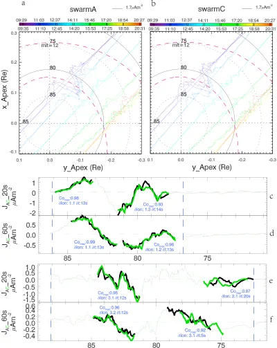
Figure 1 demonstrates the method we have adopted for data selection and the correlation analysis. Figures 1a and 1b show FACs along several Swarm orbit tracks within time period of 09:29–20:31 UT on 6 June 2014, projected onto Magnetic Apex coordinates. We can see that similar FAC signals on Swarms A and C were seen for several hours, revealing corresponding current sheets distributed over some longitudes, but slowly changing in time and orbit track. Although the signals observed by Swarms A and C are very simi-lar, differences are observed between them, even though the time delay for each spacecraft to arrive at the same apex latitude varies from a few to about 14 s, and the difference in longitude (δlon) is ~1°–3° between Swarms A and C. The total time difference between the dual-spacecraft segments of maximum correlation (bold orbit segments in Figures 1c–1f) indicates the time difference of arrival at the same current sheet,δt (see below).
To obtain the correlations of FACs observed by the two satellites we separate the regions between the mod-eled poleward and equatorward auroral boundaries (as defined by the method of Xiong & Lühr, 2014) into two broadly equal intervals predominantly containing“R1”and“R2”signals (each containing approximately the same range of latitudes). The modeled poleward and equatorward auroral boundaries on 14:30 UT 6 June 2014 are shown in Figures 1a and 1b by the magenta dashed curves. In Figures 1c–1f; however, for each orbit track the specific auroral boundaries are indicated by vertical dashed lines. The effective total time shift (δt) and the longitude difference (δlon) between the two spacecraft when the positions of the maximum correla-tions are found are denoted in each panel. Maximum correlacorrela-tions are obtained for 60-s sliding orbit segments of Swarms A and C within the R1 or R2 intervals. The segments with maximum correlation adoptedfinally are shown in Figures 1c–1f by bold traces for each spacecraft (where the maximum correlation and longitude dif-ference are indicated in blue text) with two different low-passfilters, 20 and 60 s. Thefiltering of the data defines the optimum data segments for that resolution and tests the temporal content, that is, the degree of stationarity in the data signal is expected to decrease with decreasing scale size of activity.
We use 60-s length segment windows for the correlation to get rid of any influence from variable lengths on the computation of the maximum correlations. From tests using different segment lengths, we found that using longer segments can reduce the effectiveness infinding the max-correlation between two tracks when the“R1”or“R2”contain too many points within the segments, and it also can increase the likelihood of non-regular, shorter tracks occurring, introducing systematic errors in the maximum correlations. On the other hand, segments with too few points can decrease the confidence level of the correlation. After some experi-mentation, we selected a 60-s sliding window to maximize correlations and minimize the effects of systema-tic errors. When there is less than 72 points in an orbit track we remove the track.
Figure 1.Swarm A/C FACs for an example interval on 6 June 2014, corresponding to a sequence of consecutive orbits (color coded with time from black to red shown above the color bar in (a) and (b), where (a) shows 20-sfiltered FACs observed by Swarm A plotted on the orbits within time period 09:29–20:31 UT where the FAC magnitude scale is denoted on the top-right, and (b) shows the same as (a) but for Swarm C. The model (Xiong & Lühr, 2014) poleward and equatorward auroral boundaries of current intensity on 14:30 UT are shown on Figures 1a and 1b by the magenta dashed curves. The lower panels (c to f) show two, dual spacecraft (Swarm A [black] and Swarm C [green]) intervals within this sequence, plotted as a function of apex latitude, and the current value not on the same scale: (c) and (d) show thefirst north des-cending orbit track (black orbit in panels (a) and (b)), where the R1 and R2 boundaries are estimated to be at 9:30 and 9:33 UT, and (e) and (f) are for three orbits later (light blue orbit in panels (a) and (b)) with boundaries at 14:13 and 14:18 UT. Each pair shows the 20-s (upper panels (c) and (e)) and 60-s (lower panels (d) and (f)) moving average data and also indicates the sliding maximum correlation achieved for the two intervals between R1 and R2 boundaries (blue dashed lines) with the longitude and time shift between A and C for each interval (blue text). FAC =field-aligned current.
10.1029/2018JA025205
us to study the correlation trends as a function of MLT and the differences in apex longitude or time between Swarms A and C and to define an approximate orientation of the large-scale FACs (see section 3).
3. Correlation Analysis
3.1. Current Sheet Orientation
We can see from Figure 1c–1f that the two orbits chosen show distinct situations. Thefirst shows a time delay of ~13 s between Swarms A and C, with small difference in longitude, and the FAC signals are seen at the same latitude. The second shows a different time delay in a different region (which changes for differentfi l-ters), together with a larger difference in longitude. Figures 1e–1f show a time delay in R1 of 12 s, and in R2 of 20 s (for 20-sfiltered data) and 5 s (for 60-sfiltered data). The reason for different time delays (20 s in Figure 1e and 5 s in Figure 1f in R2) is that the maximum correlations appear at different latitudes when using different low-passfilters, which select different temporal, and hence spatial, scales. The position of maximum correla-tion between Swarms A and C is obtained for two orbit segments. Thus, if we draw a line between the centers (average positions) of these segments we define the relative orientation of the satellite positions which are inferred to be at the crossing of the current sheet (sampled at A and C, respectively) in the 1-D sense. This, then, provides an estimate of the orientation of the current sheet from these relative positions. Inevitably there are influences arising from any temporal evolution of the current sheet between Swarms A and C (depending on thefiltering used; Forsyth et al., 2017; Lühr et al., 2015), such as influence arising from any pro-pagation of the current sheet during the shifted time,δt. In addition, spatial structure on the scale of the spacecraft separation will also influence the estimate (Dunlop et al., 2016, 2018). Nevertheless, the important point to note here is that for high levels of cross-correlation and hence for large-scale structures that do not significantly evolve on the scale ofδtandδlong, the estimates are more accurate, so thatfluctuations and var-iance in the orientations highlight the presence of small-scale FACs. From statistics, wefind that the 20- and 60-sfiltered data show very similar results. Thus, these current sheet orientations of R1 and R2 at 110-km alti-tude are drawn on polar maps in Figures 2a and 2b only for the 20-sfiltered data set.
It needs to be pointed out that, as mentioned earlier, we use the model estimated auroral boundaries from Xiong and Lühr (2014) here to split each auroral track into two regions, and indicate them as higher latitude regions (labeled loosely asR1in this paper) and lower latitude regions (labeled approximately asR2in this paper). Since we are using only these broad definitions of the intervals for simplicity, we expect that the R1 set actually contains other currents than purely R1 and that the R2 set contains some R1 currents in actu-ality, and indeed, there are other currents around noon. Nevertheless, from a statistical perspective we expect that the main characteristics of the large-scale currents will dominate each region. The polarity of the currents in R1/R2 also does not affect our results since we are considering only the ordering of the current sheet orien-tations (and the pattern of correlations with MLT in section 3.2).
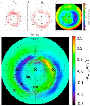
Figures 2a and 2b show inferred current sheet orientations (estimated by the method described above and as described in the caption) for each region using 20-sfiltered data from 17 April 2014 to 20 August 2014, during which time period the Swarms A and C orbits have covered the Earth for nearly a full range of 24 hr MLT. Figure 2a, denoted by R1, shows the current sheet orientations found for the higher latitude regions. Figure 2b, denoted byR2, is for the lower latitude regions. The magnitude of the longitudes (0°, 90°, 180°, and and 90°) in Magnetic Apex coordinates are denoted on eachfigure, and the latitudes in the same coor-dinates are denoted at the line of 135° longitude. The sets of line segments shown in each panel, represent-ing the current sheet orientations, are drawn for those estimates at correlation values over 0.97. At this threshold the patterns are most clearly visible and show the distinction in the ordering in each region (see below). For lower threshold values of the correlation more vectors would be included and these contain more influence from temporal and spatial effects.
current sheets for the higher latitude region is less well ordered to the oval. This suggests that the character of the poleward current sheets is less dominated by large-scale structures and that this region contains more than one current system.
[image:6.612.191.559.89.524.2]As a further check on the stability of these estimates, Figure 2c shows the comparison of these current sheet orientations to those implied for a 1-D current sheet inferred from maximum variance estimates (MVA, see Sonnerup & Scheible, 1998) of the orientations in terms of the intersection angle (the difference between the orientations for each method). The data segments for MVA were taken from those used for the maximum correlations for each Swarm A position. The current sheet orientations obtained from maximum correlation
Figure 2.(a and b) Northern hemisphere polar map, showing inferred current sheets, for Swarms A and C data from 17 April 2014 to 20 August 2014, during which time Swarm A and C’s orbit has covered 24 hr MLT. These are plotted using lines of normalized length, which connect the average Swarm A and C positions of those orbit segments producing the maximum correlations (drawn for 20-sfiltered data), where (a) shows the current sheet orientations found for the higher latitude regions; (b) shows those for the lower latitude regions; (c) shows the intersection angle of current sheets calculated by maximum correlation and MVA method, for Swarm A and C data from 17 April 2014 to 30 April 2016; and (d) shows a northern hemisphere polar map, showing the average FACs for Swarm A and C data from 17 April 2014 to 30 April 2016, overlain with similar current sheet orientations to (a) and (b) but for both higher latitude regions and lower latitude regions. FAC =field-aligned current; MLT = magnetic local time.
10.1029/2018JA025205
are quite similar to the estimates using the MVA method. The plot shows that the intersection angles of the average current alignments derived from these two methods (MVA and maximum correlation) for Swarms A and C data from 17 April 2014 to 30 April 2016, and these are all less than 0.8° (and less than this in the auroral region). The intersection angles are lowest in the dawn-side region. In fact, the difference between the two methods will arise naturally since the MVA measurement is centered on the Swarm A position, whereas the maximum correlation result is an average centering on a position midway between A and C. The correla-tion method is therefore more stable overall, but we have shown that they agree in regions where MVA is expected to behave well. The method here covers a large range. We might expect that these will agree best in regions dominated by large-scale structure and this is indeed the case although there is an asymmetry in the extent of the agreement from dawn to dusk. The close agreement on the dawn side suggests that the orientations from both methods on the dawn side are more stable over a wider range of MLT and that the effect of the differing positions is less, perhaps due to the simpler shape of the oval on the dawn side. On the other hand, the close average alignment of the maximum correlation orientations on the dusk side sug-gests that the large-scale ordering is most dominant there. Such asymmetric character from dawn to dusk is also seen in the correlation trends discussed below.
Figure 2d, denoted by R1&R2, shows the current sheet orientations for both the higher and lower latitude regions combined, superimposed on the average distribution of FACs for Swarm A from 17 April 2014 to 30 April 2016. In the underlying pattern of FACs we see the R2 and R1 up-down (in thefield-aligned sense this corresponds to negative-positive) currents as well as the Region 0 and NBZ regions near noon. This over-lay plot shows that the current sheet orientations of R1&R2 can cover the whole oval region, as well as the Region 0 and NBZ region. The alignment of the current sheets reflects the large-scale features in the polar map of average FACs closely. Although further work is required to quantify the characteristics, the mean posi-tion separating of R1 and R2 can be seen. In addiposi-tion, the cluster of differing orientaposi-tions near noon corre-sponds to the average currents seen there. The intensity of the average current does not correlate with the alignment of the sheets in general.
Further details of the FAC current sheet orientations (in particular, separating the behavior in terms of activity and other external drivers and exploring further the stability of the orientations for different correlation levels) will be discussed in future work. Here we focus simply on the R1/R2 alignment in order to compare with the correlation trends described below.
3.2. Correlation Trends
Using the methodology described in section 2 we analyzed the data from 17 April 2014 to 30 April 2016, where the spacecraft pair A-C covered a close range of both cross-track (local time longitude,δlon) and along track (time differences between the spacecraft,δt) positions (see Figure 1). The range ofδtandδlonare 0– 0.3 min along track and 0°–3° longitude (Magnetic Apex coordinates) across track. These ranges allow us to separate the cross-correlations between the spacecraft into bothδtandδlonbins independently, so as to explore the MLT dependence of the correlations. We have explored these correlations for bothfiltered and unfiltered data to understand the effect of large- (>150 km) and small- (~7.5 km) scale structures, and their trends. Thefiltered data, as discussed earlier, allow consistent comparisons on the scales of the interspa-cecraft separation (i.e., ~150 km) and above. The lower choice of 20 s matches the cadence used for the dual spacecraft FAC product in the Swarm level 2 data and therefore was used for the estimates of current sheet orientation in the previous section. It should be emphasized that it is not always possible to completely sepa-rate spatial and temporal behavior and small-scale FACs in general depend both on space and time. Nevertheless, single spacecraft FAC estimates can still be valid locally at each spacecraft within certain criteria (Lühr et al., 1996) and the Swarm products are calculated at the higher smoothed cadence of 1 s (what we termunfiltered datahere). Although some types of behavior are problematic, and the estimates can be quan-titatively in error, variations on the spacecraft separation scale can be monitored through their effect on the correlation trends. We use the single spacecraft estimates in this sense here to reveal the locations and some characteristics of the smaller-scale currents, through comparison offiltered and unfiltered signals.
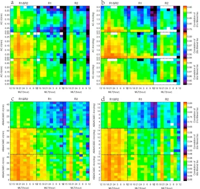
R2 interval should not only relate to actual region-2 FACs but also contain some actual R1 currents, and possibly some other currents near noon, as shown by Figure 2b. Similarly, the R1 interval will include other high-latitude current systems from time to time. Each row in the 3 × 3 arrays refers to thefiltering level applied to the data. It is instructive to consider the region separation for both unfiltered andfiltered data. Figure 3a shows the MLT trends with respect to the time delay from the Swarms A and C spacecraft. The top panels of Figure 3a show the total correlations for the unfiltered magnetic residuals, that is, those including signals from both small- and large-scale structures. The panels headed “R1” and “R2” show clearly distinct trends in both MLT andδt,δlon, which actually are broadly maintained for each of the filtered data sets, consistent with the predominant nature of these regions. The R1&R2 panel is shown for context and represents the strongest effect of the signals seen in the whole auroral and some of the polar regions.
[image:8.612.176.575.92.470.2]For the unfiltered, 1-s resolution data, the R2 correlations remain relatively high for a broad range of MLT and are obviously lower for the range 9–15 MLT (i.e., around local noon). There is also a minor dip in the strength of the correlations from 0–3 MLT (i.e., at local midnight). This trend is maintained for most of the range ofδt and is consistent with the expectation that R2 FACs are stable for a large range of MLT, centered on predawn and postdusk. The correlations on the dusk side are higher and extend for the maximum range ofδt,
Figure 3.(a) Nine panels showing vertically from the top the A-C correlation, binned with theδtdifference, as a function of MLT, for unfiltered data, 20-s low-passfiltered data and 60-s low-passfiltered data. The three columns are for
correlations over the whole interval between the R1 and R2 boundaries and for the intervals covering R1 and R2, respectively (denoted by R1&R2, R1 and R2 each at the top); (b) similar array of correlations but binned withδlon; (c and d) similar array of correlations but of A-B and B-C correlation. MLT = magnetic local time.
10.1029/2018JA025205
suggesting a dawn-dusk asymmetry in the stability of R2 FACs. This is probably associated with the high cor-respondence between particle precipitation at dusk and R2 FACs (see Korth et al., 2014). By contrast, the R1 correlations peak during the ranges 15–21 MLT and 3–9 MLT, that is, dusk and dawn, and are maintained for a smaller range ofδt. Thus, the correlations are lower (less than 0.83) for a broad range of MLT around local mid-night. These R1 correlations also peak atδtnear 0.13 mins, or 8 s, which may indicate that Pi1B waves (e.g., Arnoldy et al., 1998; Heacock, 1967) probably can be revealed by LEO satellite by this method. This will be discussed in section 3.3). These trends are consistent with the expectation that R1 FACs will be more tem-porally unstable overall, and there is some indication that at either side of noon, the signatures are more stable: The lower correlation around noon is possibly a result of the presence of other FACs, such as the NBZ currents or Region 0 currents, which also are calledcusp currents. The fact that the higher correlations extend away from noon is consistent with the average dawn-dusk signature of R1 currents, while the mini-mum postmidnight may be consistent with the presence of the diffuse aurora, which is most likely composed of field-aligned plasma sheet electrons scattered by the very low frequency whistler-mode chorus waves (Wing et al., 2013) and see the suggestions of Newell et al. (2009), Korth et al. (2014), or McGranaghan et al. (2016).
The 20- and 60-sfiltered data show similar trends, but a higher value of correlations, to those for R1 and R2 separately. This appears to suggest that the medium to large-scale FACs dominate the MLT trends, but other work has indicated this may not always be the case (McGranaghan et al., 2017; Neubert & Christiansen, 2003). We see, moreover, that the combined region R1&R2, for 20 secsfiltering maintains the combined distribution, suggesting that it is the smaller scale currents which affect the loss of correlation in the unfiltered data. Broadly, the trends with MLT for R1 and R2 are more similar for thefiltered data to each other, peaking away from both noon and midnight. This is consistent with the general pattern of large-scale FACs for both R1 and R2, which follow the well-known upward and downward pattern for a broad range of local times surrounding dawn and dusk (Iijima & Potemra, 1978). However, the 20- and 60-sfiltered data for R1 shows some additional structure, that is, the correlations sometimes (e.g., at 15–18 MLT for 20-s and 18–21 MLT for 60-sfiltered data) increase instead of decrease asδtdecrease at the lowestδt(0- to 0.05-min bins). This implies the trend modu-lated by the wave is defeated by the expected peak at lowδt, which is an obvious trend for the unfiltered correlation in Figure 3c.
The trends in Figure 3b are shown for theδlonseparation between Swarms A and C, which are different from the trends forδt. First, we see that the R1 trends are highly localized to smallδlon(0–0.5 degs) and rapidly fall off asδlonincreases. The correlations of the two highest correlated, or steadier, FACs regions, 15–21 and 3–9 MLT for R1, fall from about 0.94 to 0.78, for the unfiltered data, and ~0.995 to ~0.975 for thefiltered data. This suggests that the FAC profiles are very sensitive to shifts in longitude. This effect lessens significantly for the 20-s and 60-s data, as might be expected for larger-scale FACs. This can be attributed to the lower applicabil-ity of the infinite current sheet approximation to the small-scale currents. This also suggests that the correla-tions seen inδtare dominated by the periods when A–C have a small difference in longitude.
R2 currents exhibit similar but weak trends. After examining the number of cases in each bin, we suggest the peaks aroundδlon~ 1° are probably from the rare cases in the lowest of all valid bins (containing not less than five cases). In the“R2”region and for the 20-s data, the higher correlation trends are less sensitive to the long-itude shift, and, as revealed by Figure 2b, this is consistent with the higher degree of alignment to the oval of these current sheets.
Theδtversusδlondependence of correlations taken at different MLT regions (not shown here) demonstrates that the peak inδtseen for R1, corresponding to temporal variations of order ~8 s (as outlined above), does not come from a specific lowδlonby chance. This probably suggests that the modulation of the currents by Alfven waves is notable in the R1 region (Liu et al., 2009; Ma et al., 1995; Stasiewicz et al., 2000). In fact, we see that for the unfiltered combined interval R1&R2, nearly only the overlapping region between 18 and 21 MLT remains high (more than 0.85) and is also centered aroundδt~ 0.13 mins (8 s). We will discuss this phenom-enon in detail in section 3.3.
3.3. Pi1B Waves
The occurrence of ground based Pi1B is well documented (e.g., Arnoldy et al., 1998; Heacock, 1967). Here“B” is the abbreviation for“Burst.”Although there is evidence of both an ionospheric and magnetospheric origin, there is still no agreement on the origin of the Pi1B waves. Heacock suggested that ground PilB waves were not generated in space because of the lack of frequency dispersion in the ground events. Subsequently, sev-eral studies have shown the association of Pi1B waves with different types of ionospheric activity (Arnoldy et al., 1998, and papers therein) indicating that the waves probably result from ionospheric currentfl uctua-tions. Using magneticfield data, Arnoldy et al. (1998) showed that Pi1B waves observed by the geosynchro-nous GOES (Geostationary Operational Environmental Satellites) satellites were nearly simultaneously observed on the ground and appeared to be initiated by the dipolarization process of the nightside tail mag-neticfield at the onset of substorms. Arnoldy et al. further commented that with induction antennas sam-pling up to 10 Hz, there is indeed evidence of dispersion in the higher frequency PilB waves.
Other work has also suggested that Pi1B waves are associated with substorms, as well as FACs. Lessard et al. (2006) suggested that they were excited by reconnection or some other processes, and were compressional in nature, at least at geosynchronous orbit, implying either fast or slow mode. It should be noted that slow mode waves would be quickly damped so do not propagate to the ionosphere. However, the fast mode waves can propagate isotropically, cutting across the magneticfield obliquely in the vicinity of the GOES satellites. They noticed that at FAST (Fast Auroral Snapshot Explorer) altitudes, the waves are of shear mode, so it must have undergone mode conversion in the region between GOES 9 and FAST. They suggested it was possible that as the waves approached the higher latitude regions of the magnetosphere, they gradually became increasingly parallel to the backgroundfield, where they may take on the properties of a shear wave (a guided wave) and follow thefield lines to the ionosphere. Other models have also been suggested (Lessard et al., 2011; Pilipenko et al., 2008) to interpret how propagating compressional fast magnetosonic modes transform into running Alfvén waves.
Since Pi1B waves may change mode as they propagate, and are not well studied, it is important to investigate them at different altitudes. Under normal conditions, the curl-free part of the ionospheric, horizontal current, as well as FACs, cannot directly produce any magneticfield disturbances below the ionosphere (Fukushima, 1976), and thus, these currents are usually magnetically invisible on the ground but can be detected by satel-lites above the ionosphere. Therefore, although it is known that in general ground stations usually observe Pi1B waves between 2100 and 0200 MLT (Arnoldy et al., 1998; Posch et al., 2007), ground magnetometer data alone cannot define the ionospheric phenomena. Nevertheless, it is hard to observe ultralow frequency (ULF) waves in LEO satellites since a satellite generally moves fast at this altitude so that distinguishing the tem-poral from the spatial variations is challenging; particularly using single spacecraft measurements. The max-imum correlation method, introduced here, however, can give us the spatial and temporal variation of the FACs, so potentially providing information on Pi1B properties, which are associated with the upward (Bösinger et al., 1981) and downward (Milling et al., 2008) FACs.
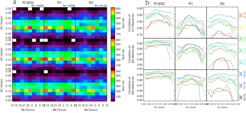
Figure 3 reveals apparent evidence of a correlation maximum around 8 s, which is about 0.13 Hz. In order to clarify this, Figure 4a represents the number of cases found in each bin of Figure 3a. Even though the data points are not equally distributed in each bin, Figure 4a only shows some overall trend for the specific orbits of Swarms A and C. The peaks around 8 s are not consistent with the Figure 4a, so do not arise from the basis time phasing between Swarms A and C (shifted by 8 s for orbit crossover). Figure 4b is another way to express the behavior shown in Figure 3a, where the correlations are no longer shown by color, but by they-axis on the left of each panel. Different colors represent different MLTs, and theδtdifference is now shown in the x-axis. Through Figure 4b, we can see the correlation peak around 0.13 min (about 8 s), nearly at all MLT, and most pronounced for the 15–21 MLT regions. Bösinger and Wedeken (1987) have mentioned that
10.1029/2018JA025205
Pi1B wave enhancement at 0.08–0.25 Hz was frequently observed at each of their six stations in both horizontal components. We note here that this is just around 4–12 s in the time domain with the center at just 8 s, as revealed by our correlation method. In contrast to the local range in longitude of the six stations mentioned in their paper, the Pi1 band phenomenon revealed by the maximum correlation method here exhibits a global property and the wave character is most obvious in R1, which is considered to map mostly to the boundary plasma sheet. Additionally, the 60-sfiltered data of R1&R2 (the lower left panel of Figure 3a) shows another peak at around 0.26 min (~16 s), which can be treated as a secondary harmonic of the 8-s wave. It is reasonable that the harmonic wave appears when the data are low-passfiltered.
Although the Pi1B waves observed on the ground have maximum amplitude when they lie underneath active auroral forms (Arnoldy et al., 1998; Bösinger & Wedeken, 1987; Danielides et al., 2001; Haldoupis et al., 1982; Milling et al., 2008), thereby suggesting they were locally generated (Posch et al., 2007). A number of studies have mentioned that Pi1B waves can extend in latitude and longitude/MLT (e.g., 12° in latitude and 20° in longitude, as mentioned by Arnoldy et al., 1998; 7°of magnetic latitude and 4 hr of MLT, as mentioned by Posch et al., 2007; 5° in latitude and less than 30° in longitude, as mentioned by Parkhomov & Rakhmatulin, 1975) For these extended distributions, only the brightest auroral onsets can be associated with Pi1B obser-vations at more than 5° in latitude and 2 hr in MLT distance. Their onsets have been seen to occur earlier at the auroral zone latitude at magnetic midnight. The horizontal ducting of wave power has been put forward, as well as the westward delay consistent with the Pi1B and initiated by the westward auroral surge were dis-cussed by Arnoldy et al. (1998), and the expansion is as rapid as 1 hr (MLT) per ~20 s (Milling et al., 2008). Currently, however, there is no report on whether Pi1B waves can expand to the dayside.
[image:11.612.176.572.93.276.2]From both Figures 3 and 4, the maximum correlations here peak around ~8 s and exhibit a global property, although they are strongest around the 15–21 MLT regions. Lee et al. (2001) has shown that impulsive FACs are strongly excited near the boundary between magnetospheric cold plasma and plasma sheet hot plasmas. This corresponds to circumstances when the Alfven speed undergoes a rapid variation, and thus, intensive shear Alfven waves can be excited through mode conversion. The indications here need further analysis to separate the effects of wave propagation and temporal amplitude variation in order to confirm the behavior. From these signals, however, we can put forward a possible scenario that either fast magnetosonic waves or shear Alfven waves (which may be generated in the boundary plasma sheet) can propagate to the iono-sphere either obliquely orfield aligned and therefore could be observed by Swarm in addition to the FACs at all MLT, with the strongest signal centering around 15–21 MLT. We cannot confirm, but it is possible that the Swarm LEO is at just the appropriate altitude for the Pi1B to spread globally and where dayside waves have not been completely damped. In turn, this may be the cause for the absence of dayside Pi1B
observations in ground-based data. This global characteristic observed by Swarm may broaden our horizon on the association of ULF waves and FACs, as well as the substorms. We will clarify this potential capability in future work.
4. Conclusions
To explore the local time dependence and stability of FACs at Swarm altitudes, we have investigated their statistical, dual-spacecraft correlation signatures between two Swarm spacecraft,flying side by side from 17 April 2014 to 30 April 2016, using a method which links the correlation intervals to model estimated oral boundaries (after Xiong & Lühr, 2014; Xiong et al., 2014). Thus, the segments are targeted relative to aur-oral boundaries defining the limit of current intensity from the ordinary R1 and R2 current systems. The interval between these boundaries is split into intervals most likely to contain R1 and R2 currents respectively. In fact, the R1 intervals cover latitudes that may contain influences from other current systems, for example, Cusp currents (Region 0), NBZ currents, and the R2 intervals may contain some ordinary R1 signals and, indeed, some other currents at noon. It is difficult to separate and distinguish these at the higher latitudes though this analysis. The unfiltered FAC data adopted here is the official Level-2 FAC data of Swarm, which is obtained by using single-spacecraft methods, which assume an infinite current sheet approximation can be applied locally to each spacecraft in the manner detailed by (Ritter et al., 2013). We have then applied 20- and 60-sfiltering to yield the low-passfiltered data and indicate the large-scale FACs (150/450 km along orbit). Cross-correlations are performed mainly on data obtained from the Swarms A and C spacecraft. The results show that the maximum correlations obtained from sliding data segments show clear trends in MLT. By connecting the average midpositions of the two intervals from Swarms A and C used to estimate the maximum correlations, we show the current sheet orientation for LEO altitude directly for thefirst time. It is obvious that the large-scale current sheets closely follow the oval on the dusk side and are also well con-sistent with the oval pattern on the dawn side and this ordering is concon-sistent with the correlation trends found. The orientations are estimated using a high (0.97) correlation level. It was noted that setting lower cor-relation thresholds for the current sheet orientations will introduce more influences from small-scale currents.
The results show that the R2 currents (referring to all FAC signatures at latitudes in the lower auroral bound-ary as defined by Xiong & Lühr, 2014) show the strongest correlations for a broad range of MLT, centered on predawn and postdusk, with a higher correlation coefficient on the dusk side and lower correlations near noon and midnight. This is consistent with the results for the current sheet alignments, where the ordering relative to the auroral oval is strongest at lower latitudes and strongest on the dusk side. The FAC profiles are very sensitive to shifts in longitude, especially for the unfiltered data, which can be attributed to the lower applicability of the infinite current sheet approximation to the small-scale currents (Forsyth et al., 2017). Correlations are much higher for thefiltered data and are more stable for up to 0.3 min, that is, 20 s, time dif-ference (δt) between Swarms A and C. It thus reflects the predominantly large-scale dominance of R2 FACs and little influence from the small-scale currents in this region. In contrast, the R1 currents (actually all high-latitude currents) peak mainly at the dawn and dusk side and are maintained for a shorter range of δt, consistent with the expectation that R1 currents are more temporally variable.
Evidence is also found for the influence from other current systems such as Region 0 and NBZ currents in the R1 region. Correlations between spacecraft A-B and B-C show littleδtorδlonsensitivity, despite persistent variabilities below 44 min, down to 0 min. This may because of the influence from different altitudes of each spacecraft, that is, 470 km, versus 531 km, which compete with theδtorδlonsensitivity. However, another possibility is the temporal stability of the large-scale FACs R1/2 FACs.
The statistical results further suggests that the higher latitude FACs are modulated by ULF waves, which seem to be Pi1B waves in the Alfven mode with a frequency of ~8 s. The trends are prominent for the unfiltered data set, indicating a relationship between the small-scale currents and the Pi1B waves. However, secondary harmonic waves seem to appear for the 60-sfiltered FAC data. This analysis illustrates a new way to reveal pulse observations using LEO satellites. This result arises from a statistical study and is hard to be found from case-by-case studies because of the fast motion of the LEO satellites. However, more work needs to be done to clarify this result.
The methodology, based on the correlation of single spacecraft estimates, was deliberately chosen to high-light the locations of small-scale influences, where these add to the larger-scale trends. Generally speaking,
10.1029/2018JA025205
therefore, this study clearly reflects the two different domains of FACs: small-scale (some tens of kilometers), which are time variable, and large-scale (>100 km), which are rather stationary. The study is very supportive of the dual-SC FAC approach introduced by Ritter et al. and explored recently by others (e.g., Dunlop, Yang, Yang, Lühr, et al., 2015). The study suggests the time shifts andfilters used in multispacecraft techniques are generally suitable for accurate determination of the FACs and perhaps allows the conditions where these break down to be further investigated. The evidence further suggests that the higher latitude FACs are modu-lated by ULF waves, which seem to be Pi1B waves in the Alfven mode with a frequency of ~8 s. The trends are prominent for the unfiltered data set, indicating a relationship between the small-scale currents and the Pi1B waves. However, secondary harmonic waves seem to appear for the 60-sfiltered FAC data. This analysis illus-trates a new way to reveal pulse observations using LEO satellites. This result arises from a statistical study and is hard to be found from case-by-case studies because of the fast motion of the LEO satellites. However, more work needs to be done to clarify this result.
References
Anderson, B. J., Takahashi, K., & Toth, B. A. (2000). Sensing global Birkeland currents with iridium® engineering magnetometer data.
Geophysical Research Letters,27(24), 4045–4048. https://doi.org/10.1029/2000GL000094
Anderson, H. R., & Vondrak, R. R. (1975). Observations of Birkeland currents at auroral latitudes.Reviews of Geophysics,13(1), 243–262. https:// doi.org/10.1029/RG013i001p00243
Arnoldy, R. L., Posch, J. L., Engebretson, M. J., Fukunishi, H., & Singer, H. J. (1998). Pi1 magnetic pulsations in space and at high latitudes on the ground.Journal of Geophysical Research,103(A10), 23,581–23,591. https://doi.org/10.1029/98JA01917
Bösinger, T., Alanko, K., Kangas, J., Opgenoorth, H., & Baumjohann, W. (1981). Correlation between PiB type magnetic micropulsations, auroras and equivalent current structures during two isolated substorms.Journal of Atmospheric and Terrestrial Physics,43(9), 933–945. https://doi.org/10.1016/0021-9169(81)90085-4
Bösinger, T., & Wedeken, U. (1987). Pi1B type magnetic pulsations simultaneously observed at mid and high latitudes.Journal of Atmospheric and Terrestrial Physics,49(6), 573–598. https://doi.org/10.1016/0021-9169(87)90072-9
Bythrow, P. F., Potemra, T. A., Erlandson, R. E., Zanetti, L. J., & Klumpar, D. M. (1988). Birkeland currents and charged particles in the high-latitude prenoon region: A new interpretation.Journal of Geophysical Research,93(A9), 9791–9803. https://doi.org/10.1029/ JA093iA09p09791
Cao, J., Duan, J., Du, A., Ma, Y., Liu, Z., Zhou, G. C., et al. (2008). Characteristics of middle- to low-latitude Pi2 excited by bursty bulkflows.
Journal of Geophysical Research,113, A07S15. https://doi.org/10.1029/2007JA012629
Cao, J.-B., Yan, C., Dunlop, M., Reme, H., Dandouras, I., Zhang, T., et al. (2010). Geomagnetic signatures of current wedge produced by fast
flows in a plasma sheet.Journal of Geophysical Research,115, A08205. https://doi.org/10.1029/2009JA014891
Danielides, M. A., Shalimov, S., & Kangas, J. (2001). Estimates of thefield-aligned current density in current-carryingfilaments using auroral zone ground-based observations.Annales de Geophysique,19(7), 699–706. https://doi.org/10.5194/angeo-19-699-2001
Dunlop, M. W., Haaland, S., Dong, X.-C., Middleton, H. R., Escoubet, C. P., Yang, Y.-Y., et al. (2018). Multi-point analysis of current structures and applications: Curlometer technique. In Electric Currents in Geospace and Beyond (Chap. 4, 20180417). Hoboken, NJ: John Wiley & Sons. https://doi.org/10.1002/9781119324522.ch4
Dunlop, M. W., Haaland, S., Escoubet, P. C., & Dong, X.-C. (2016). Commentary on accessing 3-D currents in space: Experiences from Cluster.
Journal of Geophysical Research: Space Physics,121, 7881–7886. https://doi.org/10.1002/2016JA022668
Dunlop, M. W., Southwood, D. J., Glassmeier, K.-H., & Neubauer, F. M. (1988). Analysis of multipoint magnetometer data.Advances in Space Research,8(9-10), 273–277. https://doi.org/10.1016/0273-1177(88)90141-X
Dunlop, M. W., Yang, J.-Y., Yang, Y.-Y., Xiong, C., Lühr, H., Bogdanova, Y. V., et al. (2015). Simultaneousfield-aligned currents at Swarm and Cluster satellites.Geophysical Research Letters,42, 3683–3691. https://doi.org/10.1002/2015GL063738
Dunlop, M. W., Yang, Y.-Y., Yang, J.-Y., Lühr, H., Shen, C., Olsen, N., et al. (2015). Multispacecraft current estimates at swarm.Journal of Geophysical Research: Space Physics,120, 8307–8316. https://doi.org/10.1002/2015JA021707
Forsyth, C., Rae, I. J., Mann, I. R., & Pakhotin, I. P. (2017). Identifying intervals of temporally invariantfield-aligned currents from Swarm: Assessing the validity of single-spacecraft methods.Journal of Geophysical Research: Space Physics,122, 3411–3419. https://doi.org/ 10.1002/2016JA023708
Foster, J. C., St.-Maurice, J.-P., & Abreu, V. J. (1983). Joule heating at high latitudes.Journal of Geophysical Research,88(A6), 4885–4897. https:// doi.org/10.1029/JA088iA06p04885
Friis-Christensen, E., Lühr, H., Knudsen, D., & Haagmans, R. (2008). Swarm—An Earth Observation Mission investigating Geospace.Advances in Space Research,41(1), 210–216. https://doi.org/10.1016/j.asr.2006.10.008
Fukushima, N. (1976). Generalized theorem for no ground magnetic effect of vertical currents connected with Pedersen currents in the uniform-conductivity ionosphere.Report of Ionosphere & Space Research in Japan,30(30), 35–40.
Gjerloev, J. W., & Hoffman, R. A. (2014). The large-scale current system during auroral substorms.Journal of Geophysical Research: Space Physics,119, 4591–4606. https://doi.org/10.1002/2013JA019176
Gjerloev, J. W., Ohtani, S., Iijima, T., Anderson, B., Slavin, J., & Le, G. (2011). Characteristics of the terrestrialfield-aligned current system.
Annales de Geophysique,29(10), 1713–1729. https://doi.org/10.5194/angeo-29-1713-2011
Haldoupis, C. I., Nielsen, E., Holtet, J. A., Egeland, A., & Chivers, H. A. (1982). Radar auroral observations during a burst of irregular magnetic pulsations.Journal of Geophysical Research,87(A3), 1541–1550. https://doi.org/10.1029/JA087iA03p01541
Harang, L. (1946). The meanfield of disturbance of polar geomagnetic storms.Terrestrial Magnetism and Atmospheric Electricity,51(3), 353–380. https://doi.org/10.1029/TE051i003p00353
Heacock, R. R. (1967). Two subtypes of type pi micropulsations.Journal of Geophysical Research,72(15), 3905–3917. https://doi.org/10.1029/ JZ072i015p03905
Iijima, T., & Potemra, T. A. (1976a). The amplitude distribution offield-aligned currents at northern high latitudes observed by Triad.Journal of Geophysical Research,81(13), 2165–2174. https://doi.org/10.1029/JA081i013p02165
Acknowledgments
Iijima, T., & Potemra, T. A. (1976b). Field-aligned currents in the dayside cusp observed by Triad.Journal of Geophysical Research,81(34), 5971–5979. https://doi.org/10.1029/JA081i034p05971
Iijima, T., & Potemra, T. A. (1978). Large-scale characteristics offield-aligned currents associated with substorms.Journal of Geophysical Research,83(A2), 599–615. https://doi.org/10.1029/JA083iA02p00599
Iijima, T., Potemra, T. A., Zanetti, L. J., & Bythrow, P. F. (1984). Large-scale Birkeland currents in the dayside polar region during strongly northward IMF: A new Birkeland current system.Journal of Geophysical Research,89(A9), 7441–7452. https://doi.org/10.1029/ JA089iA09p07441
Korth, H., Zhang, Y., Anderson, B. J., Sotirelis, T., & Waters, C. L. (2014). Statistical relationship between large-scale upwardfield-aligned currents and electron precipitation.Journal of Geophysical Research: Space Physics,119, 6715–6731. https://doi.org/10.1002/ 2014JA019961
Lee, D. H., Lysak, R. L., & Song, Y. (2001). Generation offield-aligned currents in the near-Earth magnetotail.Geophysical Research Letters,28(9), 1883–1886. https://doi.org/10.1029/2000GL012202
Lessard, M. R., Lund, E. J., Jones, S. L., Arnoldy, R. L., Posch, J. L., Engebretson, M. J., & et al. (2006). Nature of Pi1B pulsations as inferred from ground and satellite observations.Geophysical Research Letters,33, L14108. https://doi.org/10.1029/2006GL026411
Lessard, M. R., Lund, E. J., Kim, H. M., Engebretson, M. J., & Hayashi, K. (2011). Pi1B pulsations as a possible driver of Alfvénic aurora at substorm onset.Journal of Geophysical Research,116, A06203. https://doi.org/10.1029/2010JA015776
Liu, W., Sarris, T. E., Li, X., Elkington, S. R., Ergun, R., Angelopoulos, V., et al. (2009). Electric and magneticfield observations of Pc4 and Pc5 pulsations in the inner magnetosphere: A statistical study.Journal of Geophysical Research,114, A12206. https://doi.org/10.1029/ 2009JA014243
Lu, G., Baker, D. N., McPherron, R. L., Farrugia, C. J., Lummerzheim, D., Ruohoniemi, J. M., et al. (1998). Global energy deposition during the January 1997 magnetic cloud event.Journal of Geophysical Research,103(A6), 11,685–11,694. https://doi.org/10.1029/98JA00897 Lühr, H., Park, J., Gjerloev, J. W., Rauberg, J., Michaelis, I., Merayo, J. M. G., & Brauer, P. (2015). Field-aligned currents’scale analysis performed
with the Swarm constellation.Geophysical Research Letters,42, 1–8. https://doi.org/10.1002/2014GL062453
Lühr, H., Warnecke, J. F., & Rother, M. K. A. (1996). An algorithm for estimatingfield-aligned currents from single spacecraft magneticfield measurements: A diagnostic tool applied to Freja satellite data.IEEE Transactions on Geoscience and Remote Sensing,34(6), 1369–1376. https://doi.org/10.1109/36.544560
Ma, Z. W., Lee, L. C., & Otto, A. (1995). Generation offield-aligned currents and Alfvén waves by 3D magnetic reconnection.Geophysical Research Letters,22(13), 1737–1740. https://doi.org/10.1029/95GL01430
Marshall, J. A., Burch, J. L., Kan, J. R., Reiff, P. H., & Slavin, J. A. (1991). Sources offield-aligned currents in the auroral plasma.Journal of Geophysical Research,18(1), 45–48. https://doi.org/10.1029/90GL02674
McGranaghan, R., Knipp, D. J., Matsuo, T., & Cousins, E. (2016). Optimal interpolation analysis of high-latitude ionospheric Hall and Pedersen conductivities: Application to assimilative ionospheric electrodynamics reconstruction.Journal of Geophysical Research: Space Physics,121, 4898–4923. https://doi.org/10.1002/2016JA022486
McGranaghan, R. M., Mannucci, A. J., & Forsyth, C. (2017). A comprehensive analysis of multiscalefield-aligned currents: Characteristics, controlling parameters, and relationships.Journal of Geophysical Research: Space Physics,122, 11,931–11,960. https://doi.org/10.1002/ 2017JA024742
Merkin, V. G., Lyon, J. G., & Claudepierre, S. G. (2013). Kelvin-Helmholtz instability of the magnetospheric boundary in a three-dimensional global MHD simulation during northward IMF conditions.Journal of Geophysical Research: Space Physics,118, 5478–5496. https://doi.org/ 10.1002/jgra.50520
Milling, D. K., Rae, I. J., Mann, I. R., Murphy, K. R., Kale, A., Russell, C. T., et al. (2008). Ionospheric localisation and expansion of long-period Pi1 pulsations at substorm onset.Geophysical Research Letters,35, L17S20. https://doi.org/10.1029/2008GL033672
Neubert, T., & Christiansen, F. (2003). Small-scale,field-aligned currents at the top-side ionosphere.Geophysical Research Letters,30(19), 2010. https://doi.org/10.1029/2003GL017808
Newell, P. T., Sotirelis, T., & Wing, S. (2009). Diffuse, monoenergetic, and broadband aurora: The global precipitation budget.Journal of Geophysical Research,114, A09207. https://doi.org/10.1029/2009JA014326
Parkhomov, V. A., & Rakhmatulin, R. A. (1975).Localization and drift of Pi1B source (Issledovaniya po geomagnetizmu, aeronomii ifizike Solntsa)
(Vol. 36, pp. 131–137). Moscow: Nauka. (in Russian).
Pilipenko, V. A., Mazur, N. G., Fedorov, E. N., & Engebretson, M. J. (2008). Interaction of propagating magnetosonic and Alfvén waves in a longitudinally inhomogeneous plasma.Journal of Geophysical Research,113, A08218. https://doi.org/10.1029/2007JA012651
Pitout, F., Eglitis, P., & Blelly, P.-L. (2003). High-latitude dayside ionosphere response to Pc5field line resonance.Annales de Geophysique,21(7), 1509–1520. https://doi.org/10.5194/angeo-21-1509-2003
Pitout, F., Marchaudon, A., Blelly, P.-L., Bai, X., Forme, F., Buchert, S. C., & Lorentzen, D. A. (2015). Swarm and ESR observations of the iono-spheric response to afield-aligned current system in the high-latitude midnight sector.Geophysical Research Letters,42, 4270–4279. https://doi.org/10.1002/2015GL064231
Posch, J. L., Engebretson, M. J., Mende, S. B., Frey, H. U., Arnoldy, R. L., Lessard, M. R., et al. (2007). Statistical observations of spatial charac-teristics of Pi1B pulsations.Journal of Atmospheric and Solar - Terrestrial Physics,69(15), 1775–1796. https://doi.org/10.1016/j. jastp.2007.07.015
Rankin, R., Samson, J. C., & Tikhonchuk, V. T. (1999). Discrete auroral arcs and nonlinear dispersivefield line resonances.Geophysical Research Letters,26(6), 663–666. https://doi.org/10.1029/1999GL900058
Richmond, A. D. (1995). Ionospheric electrodynamics using magnetic apex coordinates.Journal of Geomagnetism and Geoelectricity,47(2), 191–212. https://doi.org/10.5636/jgg.47.191
Ritter, P., Lühr, H., & Rauberg, J. (2013). Determiningfield-aligned currents with the Swarm constellation mission.Earth, Planets and Space,
65(11), 1285–1294. https://doi.org/10.5047/eps.2013.09.006
Sonnerup, B. U. Ö., & Scheible, M. (1998). Minimum and maximum variance analysis.ISSI Scientific Reports Series,1, 185–220.
Stasiewicz, K., Bellan, P., Chaston, C., Kletzing, C., Lysak, R., & Maggs, J. (2000). Small-scale Alfvénic structure in the aurora.Space Science Reviews,92, 423–533. https://doi.org/10.1023/A:1005207202143
Stolle, C., Floberghagen, R., Lühr, H., Maus, S., Knudsen, D. J., Alken, P., et al. (2013). Space weather opportunities from the Swarm mission including near real time applications.Earth, Planets and Space,65(11), 1375–1383. https://doi.org/10.5047/eps.2013.10.002
Waters, C. L., & Sciffer, M. D. (2008). Field line resonant frequencies and ionospheric conductance: Results from a 2-D MHD model.Journal of Geophysical Research,113, A05219. https://doi.org/10.1029/2007JA012822
Wing, S., Fairfield, D. H., Johnson, J. R., & Ohtani, S.-I. (2015). On thefield-aligned electricfield in the polar cap.Geophysical Research Letters,42, 5090–5099. https://doi.org/10.1002/2015GL064229
10.1029/2018JA025205
Wing, S., Gkioulidou, M., Johnson, J. R., Newell, P. T., & Wang, C.-P. (2013). Auroral particle precipitation characterized by the substorm cycle.
Journal of Geophysical Research: Space Physics,118, 1022–1039. https://doi.org/10.1002/jgra.50160
Xiong, C., & Lühr, H. (2014). An empirical model of the auroral oval derived from CHAMPfield-aligned current signatures—Part 2.Annales de Geophysique,32(6), 623–631. https://doi.org/10.5194/angeo-32-623-2014
Xiong, C., Lühr, H., Wang, H., & Johnsen, M. G. (2014). Determining the boundaries of the auroral oval from CHAMPfield-aligned currents signatures—Part 1.Annales de Geophysique,32(6), 609–622. https://doi.org/10.5194/angeo-32-609-2014
Yu, Y., Cao, J., Fu, H., Lu, H., & Yao, Z. (2017). The effects of bursty bulkflows on global-scale current systems.Journal of Geophysical Research: Space Physics,122, 6139–6149. https://doi.org/10.1002/2017JA024168
Yu, Y., Ridley, A. J., Welling, D. T., & Tóth, G. (2010). Including gap regionfield-aligned currents and magnetospheric currents in the MHD calculation of ground-based magneticfield perturbations.Journal of Geophysical Research,115, A08207. https://doi.org/10.1029/ 2009JA014869
Zmuda, A. J., Heuring, F. T., & Martin, J. H. (1967). Dayside magnetic disturbances at 1100 kilometers in the auroral oval.Journal of Geophysical Research,72(3), 1115–1117. https://doi.org/10.1029/JZ072i003p01115