warwick.ac.uk/lib-publications
Original citation:
Mueller, Philippe, Stathopoulos, Andreas and Vedolin, Andrea. (2017) International
correlation risk. Journal of Financial Economics .
Permanent WRAP URL:
http://wrap.warwick.ac.uk/94014
Copyright and reuse:
The Warwick Research Archive Portal (WRAP) makes this work by researchers of the
University of Warwick available open access under the following conditions. Copyright ©
and all moral rights to the version of the paper presented here belong to the individual
author(s) and/or other copyright owners. To the extent reasonable and practicable the
material made available in WRAP has been checked for eligibility before being made
available.
Copies of full items can be used for personal research or study, educational, or not-for-profit
purposes without prior permission or charge. Provided that the authors, title and full
bibliographic details are credited, a hyperlink and/or URL is given for the original metadata
page and the content is not changed in any way.
Publisher’s statement:
© 2017, Elsevier. Licensed under the Creative Commons
Attribution-NonCommercial-NoDerivatives 4.0 International
http://creativecommons.org/licenses/by-nc-nd/4.0/
A note on versions:
The version presented here may differ from the published version or, version of record, if
you wish to cite this item you are advised to consult the publisher’s version. Please see the
‘permanent WRAP url’ above for details on accessing the published version and note that
access may require a subscription.
International Correlation Risk
✩Philippe Muellera, Andreas Stathopoulosb, Andrea Vedolina
aLondon School of Economics, Department of Finance, Houghton Street, WC2A 2AE London, UK bUniversity of Washington, Foster School of Business, 4277 NE Stevens Way, Seattle, WA 98195, USA
Abstract
We document that the cross-sectional dispersion of conditional FX correlation is countercyclical and that currencies
that perform badly (well) during periods of high dispersion yield high (low) average excess returns. We also find a negative cross-sectional association between average FX correlations and average option-implied FX correlation
risk premiums. Our findings show that while investors in spot currency markets require a positive risk premium for exposure to high-dispersion states, FX option prices are consistent with investors being compensated for the risk of
low-dispersion states. To address our empirical findings, we propose a no-arbitrage model that features unspanned FX
correlation risk.
JEL classification: F31, G15
Keywords: Correlation risk, Exchange rates, International finance
1. Introduction
It is well known that stock return correlations are countercyclical and correlation risk is priced, arguably due to the reduction of diversification benefits that occurs when stock return correlations increase. However, existing literature
has largely ignored the foreign exchange (FX) market. In this paper, we explore the properties of FX correlations using both spot and options market data and we propose a reduced-form no-arbitrage model that is consistent with our
empirical findings.
First, we document the empirical properties of conditional FX correlations. We consider exchange rates against
the U.S. dollar (USD) and show that there exists substantial cross-sectional heterogeneity in the average conditional correlation of FX pairs. Furthermore, using several business cycle proxies, we find that the cross-sectional dispersion
of FX correlations is countercyclical: FX pairs with high (low) average correlation become more (less) correlated in adverse economic times. We exploit the cyclical properties of conditional FX correlation by defining an FX
correlation dispersion measure, FXC, and sort currencies into portfolios based on the beta of their returns with respect to innovations in FXC, denoted by∆FXC. We find that currencies with low∆FXC betas have high average excess
returns, whereas currencies with high∆FXC betas yield low excess returns, suggesting that FX correlation risk has
a negative price in spot FX markets. In particular, in our benchmark sample of G10 currencies, H MLC, a currency
portfolio with a short position in the high∆FXC beta currencies and a long position in the low∆FXC beta currencies,
generates a highly significant average annual excess return of 6.42% with a Sharpe ratio of 0.82.
✩We would like to thank Dante Amengual, Andrew Ang, Svetlana Bryzgalova, Joe Chen, Mike Chernov, Ram Chivukula, Max Croce, Robert
Dittmar, Dobrislav Dobrev, Anh Le, Angelo Ranaldo, Paul Schneider, Ivan Shaliastovich, Adrien Verdelhan, Hao Zhou, and seminar and conference participants of LUISS Guido Carli, Rome, University of Lund, University of Piraeus, University of Bern, Stockholm School of Economics, Federal Reserve Board, University of Essex, London School of Economics, Ohio State University, Southern Methodist University, University of Pennsylvania (Wharton), Bank of England, Chicago Booth Finance Symposium 2011, 6th End of Year Meeting of the Swiss Economists Abroad, Duke/UNC Asset Pricing Conference, UCLA-USC Finance Day 2012, the Bank of Canada–Banco de Espa˜na Workshop on “International Financial Markets”, Financial Econometrics Conference at the University of Toulouse, SED 2012, the 8th Asset Pricing Retreat at Cass Business School, the CEPR Summer Meeting 2012, the EFA 2012, and the AEA 2016 for thoughtful comments. Philippe Mueller and Andrea Vedolin acknowledge financial support from STICERD, the Systemic Risk Centre at LSE and the Economic and Social Research Council (Grant ES/K002309/1).
We continue our empirical investigation by using currency option prices to extract conditional FX correlation dynamics under the risk-neutral measure. We calculate FX correlation risk premiums, defined as the difference between
conditional FX correlations under the risk-neutral measure and the physical measure, and we find a strongly negative
cross-sectional association between average FX correlations and average FX correlation risk premiums: FX pairs characterized by low (high) average correlations tend to exhibit positive (negative) correlation risk premiums. Thus, the
cross-sectional dispersion of FX correlations is on average lower under the risk-neutral measure than under the physical measure. We also document a very strong negative time-series association between FX correlations and FX correlation
risk premiums for almost all FX pairs. As regards cyclicality, FX pairs with high average correlation risk premiums have countercyclical correlation risk premiums, whereas pairs with low correlation risk premiums have procyclical
premiums. Thus, bad states amplify the magnitude of FX correlation risk premiums, increasing their cross-sectional dispersion.
We rationalize our empirical findings with a no-arbitrage model of exchange rates. The main tension we address is between the physical and the risk-neutral measure FX correlation dynamics. Under the physical measure, the negative
association between∆FXC betas and currency returns suggests that U.S. investors require a positive risk premium for
being exposed to states in which the cross section of FX correlations widens. However, FX options are priced in a
way that suggests that U.S. investors worry about states in which the cross section of FX correlations tightens, as the risk-neutral measure FX correlation dispersion is on average lower than its physical measure counterpart. To address
this apparent contradiction, we propose a model in which FX correlation risk is not spanned by exchange rates: the pricing kernel of U.S. investors is exposed to shocks that affect conditional FX correlations, but not exchange rates
themselves.
In the model, each country’s stochastic discount factor (SDF) is exposed to two global shocks, as well as a single country-specific shock. Importantly, countries have heterogeneous loadings on the first global shock, but identical
loadings on the second global shock. As a result, the absence of arbitrage in international financial markets suggests that exchange rates are exposed only to the first global shock, whereas the second global shock cancels out and does not
affect exchange rates at all. The steady-state cross-sectional distribution of conditional FX correlations is determined by the cross section of exposures to the first global shock: on average, the USD exchange rates of foreign countries with
similar exposure to the first global shock (called similar FX pairs) are more correlated than FX pairs of countries with dissimilar global risk exposure (called dissimilar FX pairs). Crucially, the cross section of conditional FX correlations
exhibits time variation due to the fact that conditional FX correlations are determined by the relative importance of country-specific risk and global risk, which varies over time. When the relative magnitude of country-specific SDF
shocks increases, the countries’ heterogeneous exposure to the first global shock becomes less important quantitatively, and the cross section of conditional FX correlations tightens, with high correlation FX pairs becoming less correlated
and low correlation FX pairs more correlated. Conversely, a relative increase in the magnitude of global risk increases the correlation of similar FX pairs and decreases the correlation of dissimilar FX pairs, widening the cross section of
conditional FX correlations.
In turn, the relative magnitude of country-specific and global risk is determined by the relative magnitude of the local pricing factor, which prices country-specific risk and is exposed to the second global shock, and the global
pricing factor, which prices global risk and is exposed to the first global shock. When the second global shock has an adverse realization, the local pricing factor increases, tightening the cross section of conditional FX correlations;
conversely, when the second global shock has a positive realization, the cross section of conditional FX correlation becomes more dispersed. The reverse occurs for realizations of the first global shock: its adverse (positive) realizations
increase (decrease) the global pricing factor, widening (tightening) the cross section of FX correlations. Thus, the cross section of conditional FX correlations is driven by both global shocks. In the model, both shocks are priced,
but not symmetrically: U.S. investors price the second shock more severely than the first, so they attach a high price to states characterized by large relative values of the local pricing factor. Since those are exactly the states in which
As regards spot FX markets, recall that exchange rate risk does not span FX correlation risk, as exchange rates are unaffected by the second global shock. This lack of spanning allows our model to generate a negative relation between
∆FXC betas and currency returns: investing in exchange rates draws compensation solely for exposure to the first
global shock and, since negative realizations of that shock lead to a widening of the cross section of FX correlations, investors require high returns for holding negative∆FXC beta currencies, which depreciate when the cross section of
conditional FX correlations becomes more dispersed.
In sum, conditional FX correlation, which can be indirectly traded using currency options, is exposed to two
global shocks. U.S. investors price the second global shock more severely than the first one, so FX correlation risk premiums reflect the desire of currency option holders to primarily avoid states with negative realizations of the
second shock—those are the states characterized by a tightening of the cross-sectional dispersion of FX correlation, and currency option prices reveal that feature. On the other hand, investing in foreign currency exposes investors only
to the first global shock, so currency risk premiums reflect solely FX investors’ desire to avoid the corresponding bad states—those states are characterized by a widening of the cross-sectional dispersion of FX correlation, and currency
risk premiums compensate investors for exposure to those states. Thus, it is the lack of spanning of FX correlation risk by exchange rates and currency returns, and in particular the lack of exposure of exchange rates to the second global
shock, that allows our model to jointly address the empirical properties of FX correlations, currency risk premiums and FX correlation risk premiums.
A simulated version of our model generates realized FX correlations, implied FX correlations and FX correlation
risk premiums that match the cross-sectional and time-series properties of their empirical counterparts, all the while fitting the standard exchange rate, interest rate and inflation moments.
Related literature: This paper is part of the literature addressing the salient empirical properties of FX markets. Our model builds on the work of Lustig, Roussanov and Verdelhan (2011, 2014) and Verdelhan (2015); their models feature
global SDF shocks, common across countries, and local SDF shocks, independent across countries. Importantly, they assume that the price of country-specific shocks is uncorrelated across countries, as local pricing factors are perfectly
negatively correlated with the corresponding country-specific shocks. We show that allowing for cross-country comovement of the local pricing factors is crucial for explaining the joint behavior of FX correlations under the physical
and the risk-neutral measure.
Our model assumes ex ante heterogeneity across countries regarding their exposure to global shocks. Recent international finance models that address the cross section of currency risk premiums by assuming ex ante heterogeneity
across countries include Hassan (2013), Tran (2013), Backus, Gavazzoni, Telmer and Zin (2013), Colacito and Croce (2013), Colacito, Croce, Gavazzoni and Ready (2015), and Ready, Roussanov and Ward (2016). In all models, high
(low) interest rate currencies are risky (hedges) because they depreciate (appreciate) in bad global states. This is because high interest rate countries are those with low exposure to global risk: small countries, countries with smooth
non-traded output, countries with very procyclical monetary policy, commodity producers, or countries with low exposure to global long-run endowment shocks, depending on the model.
Finally, our paper is related to the literature on currency options. Whereas most of that literature focuses on crash risk,
especially in the context of the FX carry trade—see, for example, Farhi, Fraiberger, Gabaix, Ranciere and Verdelhan (2015), Jurek (2014) and Chernov, Graveline and Zviadadze (2016)—our aim is to use option prices to study the
properties of FX correlation risk premiums.
The rest of the paper is organized as follows. Section 2 describes the data. Section 3 reports our empirical findings
regarding the cross-sectional and time-series properties of FX correlations, as well as the pricing of correlation risk in currency markets. Our empirical findings concerning FX correlation risk premiums are presented in Section 4.
Section 5 introduces our no-arbitrage model, and Section 6 concludes. The Appendix contains details on the construction of the realized and implied FX correlation measures, results on the price of FX correlation risk, and
2. Data
Our benchmark sample period starts in January 1996 and ends in December 2013, and is dictated by the availability of the currency options data.
Spot and forward exchange rates: To calculate physical measure FX moments, we use daily spot exchange rates
from WM/Reuters obtained through Datastream. From the same source, we also collect one-month forward rates to calculate forward discounts.
Following the extant literature (see, e.g., Fama, 1984), we work with log spot and log one-month forward exchange rates, denoted si
t = ln(Sit) and fti = ln(Fit), respectively; both are expressed in units of foreign currency per USD.1 We use the U.S. dollar as the base currency, so superscript i always denotes the foreign currency. Monthly log excess returns from holding the foreign currency i are computed as rxi
t+1 = f i
t −sit+1. Our benchmark sample comprises the
nine G10 foreign currencies (AUD, CAD, CHF, EUR, GBP, JPY, NOK, NZD, SEK) from January 1996 to December 2013. For robustness checks, we also consider the longer January 1984 to December 2013 sample period. Before the
introduction of the EUR in January 1999, we use the German Mark (DEM) in its place.
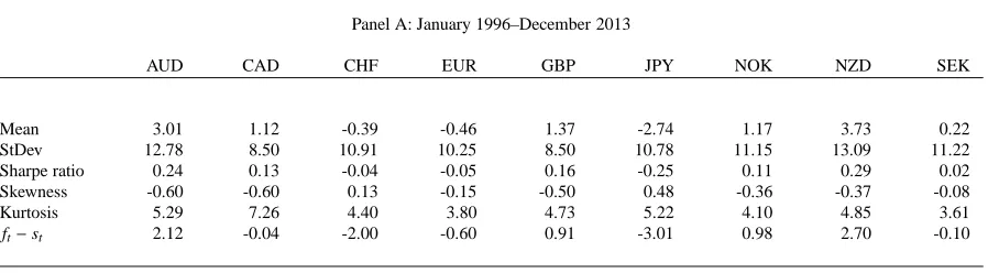
Table 1 presents the properties of the G10 currency excess returns. In line with the literature on the FX carry trade,
we find that currencies with high (low) nominal interest rates tend to yield high (low) average dollar excess returns: the NZD and the AUD are characterized by high nominal interest rates, as well as high average excess returns, while the
reverse is true for the JPY and the CHF.
[Insert Table 1 here.]
For robustness, we extend the cross section of currencies and consider two additional currency sets: developed and emerging market currencies. The developed country sample, apart from the G10 currencies, includes the currencies
of Austria, Belgium, Denmark, Finland, France, Greece, Italy, Ireland, Netherlands, Portugal, and Spain. The full sample includes all the developed country currencies, along with the currencies of the Czech Republic, Hungary,
India, Indonesia, Kuwait, Malaysia, Mexico, Philippines, Poland, Singapore, South Africa, South Korea, Taiwan, and Thailand.2
Currency options: We use daily over-the-counter (OTC) G10 currency options data from J. P. Morgan. In addition to the nine currency pairs versus the U.S. dollar, we also have options data for all 36 cross rates. The options used in this
study are plain-vanilla European calls and puts, with five option series per currency pair. Specifically, we focus on the one-month maturity and a total of five different strikes: at-the-money (ATM), 10-delta and 25-delta calls, as well as
10-delta and 25-delta puts.
3. Exchange rate correlations
In this section, we document that the cross-sectional dispersion of conditional FX correlation is countercyclical.
Following that observation, we construct an FX correlation dispersion measure, FXC, and sort currencies into portfolios based on their return exposure to FXC innovations, denoted by ∆FXC. We find a negative association
between ∆FXC betas and currency excess returns, suggesting that currency exposure to FX correlation risk is
compensated with a positive risk premium.
3.1. Properties of exchange rate correlations
We use daily spot exchange rates to calculate conditional FX correlations under the physical measure. In particular,
we proxy the conditional one-month correlation of each FX pair at time t with its realized correlation over a rolling
1WM/Reuters forward rates are available from 1997 onwards. For 1996, we either use forward rates from alternative sources or we construct
‘implied’ forward rates using the interest rate differential between the U.S. and the foreign country using interest rate data from Datastream, exploiting the fact that covered interest rate parity holds during normal conditions. We verify that our results are robust to using the WM/Reuters data only.
2We start with the same set of currencies used in Lustig, Roussanov and Verdelhan (2011). However, we exclude some currencies, such as the
three-month window of past daily observations. Appendix A provides the details. In the remainder of the paper, we will often refer to physical measure conditional FX correlation as realized FX correlation, to distinguish it from the
option-implied risk-neutral measure FX correlation (implied FX correlation).3
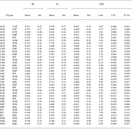
The first two columns of Table 2 report the time-series mean and standard deviation of the conditional FX correlation of each of the 36 G10 FX pairs. The mean conditional correlation is positive for all 36 FX pairs, indicating that all
pairs of USD exchange rates exhibit positive comovement on average. The cross-sectional average of the conditional correlation means is 0.45, but there is substantial cross-sectional heterogeneity: the means range from almost zero
(CAD/JPY with 0.05, indicating that fluctuations in the relative price of the CAD and the JPY against the USD
are almost disconnected), to almost one (CHF/EUR with 0.89).4 Furthermore, conditional FX correlations exhibit considerable variability across time: the cross-sectional average of the standard deviation of conditional FX correlations
is 0.23, ranging from 0.09 (EUR/NOK pair) to 0.34 (AUD/JPY pair), suggesting non-trivial swings in the degree of exchange rate comovement across time for all FX pairs.
[Insert Table 2 here.]
Given the time variation in conditional FX correlations, it is worth exploring whether that time variation is cyclical and, if so, whether there is any cross-sectional heterogeneity in its properties. To that end, we consider the comovement
of conditional FX correlations with market variables that are well-known to exhibit countercyclical behavior. The market variables we consider are a global equity volatility measure (GVol), a global funding illiquidity measure (GFI),
the TED spread (T ED), and the VIX (V IX). GVol is constructed as in Lustig, Roussanov and Verdelhan (2011). GFI is constructed following the methodology of Hu, Pan and Wang (2013), but calculated using an international sample
of government bond securities as in Malkhozov, Mueller, Vedolin and Venter (2016). T ED is the spread between the three-month USD LIBOR and the three-month Treasury Bill rate and is available in FRED. V IX is backed out from
options on the S&P 500 stock index and available from the CBOE. T ED and V IX are U.S.-specific measures, but are often used as global market indicators. GVol and GFI are calculated using international data in local currencies.
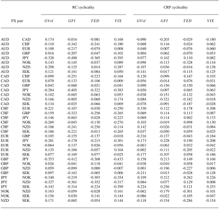
For each FX pair and each market measure, we define the cyclicality measure to be the unconditional correlation of the market variable with the conditional correlation of the FX pair. Thus, we calculate four FX correlation cyclicality
measures for each exchange rate pair, each corresponding to a market variable. We present the cyclicality measures for the 36 G10 FX pairs in the first four columns of Table 3.
[Insert Table 3 here.]
As seen in the table, we find substantial cross-sectional heterogeneity regarding the cyclicality properties of conditional FX correlations. To determine whether there is a cross-sectional pattern, we plot each cyclicality measure
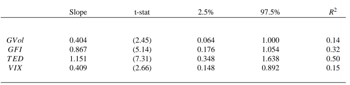
of the 36 FX pairs against their average conditional correlation; Panels A to D in Figure 1 present the plots for the four cyclicality measures. Each panel also presents the line of best fit from the corresponding cross-sectional regression.
We report the details of the four cross-sectional regressions in Panel A of Table 4: for each regression, we document the point estimate of the slope coefficient, its asymptotic t-statistic, and the 95% bootstrapped confidence interval (2.5
and 97.5 bootstrap percentiles), as well as the regression R2. The asymptotic t-statistic is calculated using White (1980)
standard errors that adjust for cross-sectional heteroskedasticity, while the bootstrapped confidence interval accounts
3For robustness, we also proxy the conditional one-month correlation of each FX pair at time t with its realized correlation over a rolling
one-month window of past daily observations, as well as with its realized correlation during the one-month ahead period, i.e. from t to t+1. Our empirical results are robust to those alternative specifications. We report some of our findings for correlation risk premiums using the alternative realized correlation proxies in the Online Appendix.
4Beginning September 2011, the Swiss National Bank imposed a cap in the relative value of the CHF by establishing a floor of 1.2 CHF per
for potential small sample effects. All four slope coefficients are positive and statistically significant at the 5% level using either the asymptotic or the bootstrapped distribution, suggesting a positive cross-sectional association between
average conditional FX correlation and FX correlation cyclicality. Indeed, Figure 1 shows that the FX pairs with high
average correlation tend to exhibit countercyclical correlations, whereas the FX pairs with low average correlation are characterized by procyclical FX correlations.5
[Insert Figure 1 and Table 4 here.]
Our findings imply that in periods characterized by adverse economic conditions or market stress, the cross section of conditional FX correlations widens, as high correlation FX pairs become more correlated and low correlation FX pairs
become less correlated. To further explore the time-series properties of the cross-sectional dispersion in conditional FX correlation, we construct a conditional FX correlation dispersion measure, called FXC, as follows: each period t,
we sort all FX pairs in deciles on their conditional correlation, calculate the average conditional correlation for the top and bottom deciles (which consist of four FX pairs each), and take the difference between the top and the bottom decile
averages to be our dispersion measure at t, FXCt. Due to the time variation in conditional FX correlations, there is turnover in both the top and bottom deciles; to eliminate composition effects, we also compute an alternative dispersion
measure (FXCUNC) by considering top and bottom deciles of FX pairs formed using average conditional correlations.
We plot the time series of the level of the two FX correlation dispersion measures in Panel A of Figure 2.6 The correlation between FXC and FXCUNC is 0.86, indicating that the two measures are very similar. Indeed, during the
financial crisis the two measures are almost perfectly correlated, as there is little turnover in the extreme deciles of FX conditional correlation. To evaluate the cyclicality properties of the FX correlation dispersion measures, we explore
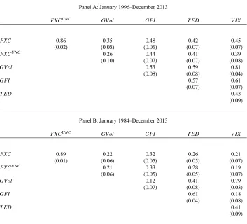
their association with the market variables we use to measure the cyclicality of FX correlations. For reference, in Panel B of Figure 2 we plot the (standardized) market variables. Panel A of Table 5 reports the unconditional correlations
between our two FX correlation dispersion measures and the market variables, in the January 1996 to December 2013 sample period, along with their bootstrap standard errors. Both dispersion measures—FXC and FXCUNC—have a
positive correlation with all four market variables; in all eight cases, bootstrap confidence intervals (which account for non-normality in small samples and are not reported in Table 5) indicate that the correlation is statistically significant
at the 1% level. Panel B repeats the same exercise for the longer January 1984 to December 2013 period; again all eight correlations of interest are positive and significant at the 1% level.
[Insert Figure 2 and Table 5 here.]
3.2. Correlation risk and the cross section of currency returns
We can now explore how exposure to FX correlation risk relates to currency returns. To do so, we sort currencies into portfolios based on the exposure (beta) of currency excess returns to innovations in our dispersion measure FXC;
innovations between t and t+1 are denoted by∆FXCt+1and are defined as the average of changes (first differences)
in conditional FX correlation for the FX pairs that belong to the top decile in period t minus the corresponding average
for the bottom decile.7 Our currency portfolios are rebalanced monthly: each month t we calculate rolling∆FXC
return betas using the last 36 monthly observations. Hence, each month t currency portfolios are formed using only
information available at time t.
We sort the nine G10 currencies into three portfolios; the first portfolio (Pf1C) contains the currencies with the
lowest∆FXC betas while the last portfolio (Pf3C) contains the highest∆FXC beta currencies. Of particular interest
5We also calculate the cross-sectional correlation coefficient between average FX correlations and each of the four cyclicality measures; the
cross-sectional correlation coefficients are 0.37 for GVol, 0.57 for GFI, 0.70 for TED and 0.38 for VIX.
6The Online Appendix presents additional results using alternative construction methods for FXC. We find that our portfolio results are robust
to those alternative specifications.
7Innovations in FXC are not the first differences in FXC, as the composition of the deciles changes over time. On the other hand, since the FX
is the H MLC portfolio, which takes a long position in Pf3Cand a short position in Pf1C. Panel A of Table 6 reports
the summary statistics for the three∆FXC-beta-sorted currency portfolios, as well as the H MLC portfolio. Notably,
average portfolio returns are monotonically decreasing in the∆FXC beta:∆FXC is a priced currency risk factor. As a
result, the average return to H MLCis negative and highly statistically significant: shorting the H MLCportfolio yields an annualized average excess return of 6.42% with a t-statistic of 3.47, and an associated Sharpe ratio of 0.82.
[Insert Table 6 here.]
Our finding of a strongly negative return for H MLCis robust to different sample periods. In particular, we consider following periods: January 1996 to July 2007, January 1984 to December 2013, and January 1984 to July 2007;
two of those periods end before the recent financial crisis. Our findings are reported in Panels B to D of Table 6. Consistent with our results for the benchmark period, we find an inverse relation between exposure to the FX correlation
factor∆FXC and average currency portfolio excess returns in each of the three periods. Excluding the financial crisis
increases the average excess return of shorting the H MLC portfolio to 7.35%, with an associated Sharpe ratio of
1.10 (Panel B). On the other hand, return differences across portfolios somewhat attenuate when the sample period is extended back to January 1984 (Panels C and D), but shorting the H MLC portfolio still yields highly significant
annualized average excess returns (3.72% and 3.45%, respectively). Overall, our results are very robust to different sample periods and do not appear to be driven by the recent financial crisis.
For further robustness, we also explore extended cross sections of currencies: in particular, we consider a sample
that includes other developed country currencies (called the developed country sample) and a sample that includes the entirety of the developed sample and also some emerging currencies (called the full sample).8 For each of the two
extended samples, we construct four∆FXC-beta-sorted portfolios. Figure 3 presents the average excess returns of
∆FXC-beta-sorted currency portfolios for each of three sets of currencies (G10, all countries and developed countries)
and each of the four periods discussed above. We find a consistently negative association between average portfolio excess returns and exposure to correlation risk, with negative average H MLC returns across the board. Furthermore,
average H MLC returns are significant at the 5% level for all currency and period samples, with the sole exception of the samples starting in 1984 for the full set of currencies. For the benchmark period from January 1996 to December
2013, the average annualized return of shorting H MLC in the developed country sample is 5.46% (with a t-statistic of 2.42) and the associated Sharpe ratio is 0.57. For the full cross section of currencies, shorting H MLCyields 4.04% on
average (with a t-statistic of 1.97) and a Sharpe ratio of 0.46.
[Insert Figure 3 here.]
Finally, given the significant excess returns to the H MLC portfolio, we attempt to determine the market price of
FX correlation risk. We follow the extant literature and consider a linear pricing model with two traded factors: the first factor is the dollar factor DOL, defined as the simple average of all available FX excess returns and shown by
Lustig, Roussanov and Verdelhan (2011) to act as a level factor for currency returns, and the second factor is H MLC,
the return difference between the high and low∆FXC beta portfolios for the sample of G10 currencies. Our estimates
for the market price of H MLC range from
−51 to−67 basis points per month, depending on the set of test assets, so
H MLCacts as a slope factor for pricing currency risk. The results are presented in detail in Appendix B.
4. Exchange rate correlation risk premiums
In this section, we document the cross-sectional and time-series properties of FX correlation risk premiums (CRP)
and explore the relation between FX correlation risk premiums and FX correlations.
4.1. The cross-sectional properties of correlation risk premiums
In consistence with the literature on variance and correlation risk premiums in other asset classes, we define FX correlation risk premiums as the difference between expected conditional FX correlations under the risk-neutral (Q) and the physical (P) measure:
CRPi,jt,T ≡EQt
Z T
t
ρi,ujdu
!
−EPt
Z T
t
ρi,ju du
!
. (1)
We only consider one-month premiums, i.e. T =t+1, as the maturity of the FX options we use to derive risk-neutral
measure moments is one month.9
To calculate the risk-neutral (implied) conditional FX correlation, we follow the literature on model-free measures
of implied volatility and covariance using daily FX option prices. The details of the calculations are presented in Appendix C. Given the availability of FX options, we calculate correlation risk premiums for each of the 36 FX pairs
formed using the nine G10 exchange rates against the USD. For each FX pair not involving the EUR, our sample period starts in January 1996 and ends in December 2013, for a total of 216 monthly observations. For the EUR, the options
data start in January 1999.
The time-series mean and standard deviation of the implied FX correlations of each of the 36 G10 FX pairs are
reported in Table 2. The cross-sectional average of implied FX correlation means is 0.48, slightly higher than its physical measure counterpart (0.45). Importantly, there is less heterogeneity in conditional FX correlation means
under the risk-neutral measure than under the physical measure: the lowest implied FX correlation mean is 0.14 (CAD/JPY pair) and the highest is 0.88 (CHF/EUR pair), whereas realized correlation means range from 0.05 to 0.89.
The volatility of implied FX correlations is of the same order of magnitude as the volatility of realized FX correlations, with standard deviations ranging from 0.07 to 0.34 and their cross-sectional average being 0.19.
Finally, the last five columns of Table 2 present the descriptive statistics for FX correlation risk premiums. From left to right, we report the time-series mean and standard deviation of the correlation risk premium of each FX pair,
followed by the asymptotic t-statistic and the bootstrapped 95% confidence interval of the CRP mean. CRP means exhibit considerable cross-sectional heterogeneity, with their size and sign varying greatly across FX pairs: they range
from−0.069 (CAD/SEK) to 0.099 (JPY/NOK), with the cross-sectional average being 0.016. Roughly two thirds of CRP means are positive and one third are negative; overall, three quarters of the means are significant at the 5% level
according to either the asymptotic or the bootstrapped distribution.10 Furthermore, correlation risk premiums are very
volatile: despite the fact that premiums are much smaller than either realized or implied FX correlations, CRP standard deviations are of the same order of magnitude as those of realized or implied correlations (ranging from 0.06 to 0.22,
with a cross-sectional average of 0.14), suggesting that there is substantial time variation in the disparity between physical measure and risk-neutral measure FX correlations.
To explore whether average FX correlation risk premiums exhibit a cross-sectional pattern, we plot the average CRP of all G10 exchange rate pairs against their average realized correlations. Figure 4 presents the scatterplot, along
with the line of best fit. The cross-sectional correlation between average FX correlation risk premiums and average FX realized correlations is−0.55. For example, the AUD/JPY pair, characterized by a very low average realized FX
correlation (0.16), has a positive and highly significant average CRP of 0.083. On the other hand, the AUD/NZD pair has a very high average realized correlation (0.76) and a negative and significant average premium (−0.016). A
cross-sectional regression of average correlation risk premiums on average realized correlations yields a statistically significant slope coefficient of−0.144.11 The strongly negative cross-sectional association between average realized
9Variance risk premiums are defined analogously as the difference in expected conditional FX variance between the risk-neutral and the physical
measure. A brief discussion of their summary statistics, as well as the summary statistics of physical measure (realized) and risk-neutral measure (implied) FX variance, is deferred to the Online Appendix. Inter alia, FX variance is studied in Cenedese, Sarno and Tsiakas (2014), who find that a high cross-sectional average of currency excess return variance predicts carry trade losses.
10In terms of size, the maximum FX correlation risk premium we find is about half of the equity correlation risk premium reported by
Driessen, Maenhout and Vilkov (2009).
11Its asymptotic t-statistic, calculated using White (1980) standard errors, is
FX correlations and average FX correlation risk premiums is what generates the tighter cross-sectional distribution of average implied FX correlations versus that of realized FX correlations that we discussed earlier.
[Insert Figure 4 here.]
The relative tightness of the cross-sectional distribution of conditional FX correlation under the risk-neutral measure
implies a potential tension regarding the pricing of FX correlation risk. On the one hand, the negative association between∆FXC betas and currency excess returns suggests that U.S. investors require a risk premium for being exposed
to states in which FXC increases, i.e. in which the cross section of FX correlations widens. However, FX options are priced in a way that indicates that U.S. investors price states in which the cross section of FX correlations tightens. In
the next section, we will address this tension by proposing a no-arbitrage model that features unspanned FX correlation risk.
4.2. The time-series properties of correlation risk premiums
We now turn to the time-series properties of implied FX correlations and FX correlation risk premiums. The first
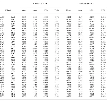
four columns of Table 7 provide summary statistics on the time-series association between realized and implied FX correlations: for each FX pair, we report the unconditional correlation coefficient between the two time series, as well
as its asymptotic t-statistic and its 95% bootstrapped confidence interval. Realized and implied correlations exhibit substantial comovement across time for all FX pairs, with the unconditional correlations between the two ranging from
0.28 to 0.92, all being statistically significant, and the cross-sectional mean being 0.79.
[Insert Table 7 here.]
The last four columns of Table 7 report descriptive statistics on the unconditional correlation between realized FX correlations and FX correlation risk premiums. We find that the cross-sectional average of those unconditional
correlation coefficients is −0.52 across the 36 G10 FX pairs, suggesting that elevated FX correlation is typically associated with lower than usual CRP, i.e., with a lower than usual disparity between the physical measure and the
risk-neutral measure FX correlation. This association is pervasive and robust: 35 of the 36 unconditional correlation coefficients are negative, with all but one of them being statistically significant.
Finally, to assess the cyclicality of correlation risk premiums, we construct CRP cyclicality measures. As we did for FX correlations, we define our CRP cyclicality measures to be the unconditional correlations between FX
correlation risk premiums and the four market variables we used before. The last four columns of Table 3 report the four CRP cyclicality measures for each of the 36 G10 FX pairs, and Panels A to D of Figure 5 plot those cyclicality
measures against average FX correlation risk premiums. We find a positive cross-sectional association: FX pairs with high average CRP have countercyclical correlation risk premiums, whereas pairs with low average CRP have
procyclical premiums. The regression results in Panel B of Table 4 suggest that this positive cross-sectional association is statistically significant for all four cyclicality measures.12Thus, the cross-sectional dispersion in FX correlation risk
premiums is countercyclical: in bad times, the premiums of FX pairs with high average CRP increase and the premiums of FX pairs with low average CRP decline, widening the cross-sectional distribution of FX correlation risk premiums.
[Insert Figure 5 here.]
5. A no-arbitrage model of exchange rates
In this section, we introduce a reduced-form, no-arbitrage model of exchange rates that is consistent with our
empirical findings. Our model builds on the reduced-form models in Lustig, Roussanov and Verdelhan (2011, 2014)
12We also calculate the cross-sectional correlation coefficient between average CRP and each of the four CRP cyclicality measures; the
and Verdelhan (2015). In contrast to those models, which assume that innovations in the price of country-specific shocks are uncorrelated across countries, we assume that local risk is priced identically across countries. This
assumption implies a lack of spanning of FX correlation risk by exchange rates, a feature that is crucial in jointly
explaining the behavior of FX correlations and FX correlation risk premiums.
5.1. Model setup
The global economy comprises I+1 countries (i=0,1, . . . ,I), each with a corresponding currency. Without loss of
generality, we will call country i=0 the domestic country and countries i=1, ...,I the foreign countries. We assume
that financial markets are frictionless and complete, so that there is a unique stochastic discount factor (SDF) for each
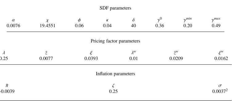
country, but that frictions in the international market for goods induce non-identical stochastic discount factors across countries. In particular, the log SDF of country i, denoted by mi, is exposed to two global shocks, uw and ug, and a
country-specific (local) shock ui, and satisfies
−mit+1=α+χzt+ϕzwt +
√κz
tuit+1+
q
γizw
tu w t+1+
p
δztu
g
t+1, (2)
where z and zwis the local and the global pricing factor, respectively. Both pricing factors are common to all countries.
Notably, countries are ex ante heterogeneous only with regard to their exposureγto the first global shock uw; all other SDF parameters are identical across countries. As we will see, differences inγcapture an exchange rate fixed effect
that generates, inter alia, cross-sectional differences in average FX correlations. In our model, global risk exposureγ is exogenous.13.
The local pricing factor z prices both the local shock uiand the second global shock ug: in all countries, the price of the local shock is √κztand the price of the second global shock is
√
δzt. On the other hand, the first global shock uwis differentially priced across countries, with its price in country i being pγizw
t.
The two pricing factors are stationary processes. The local pricing factor z is driven by the second global shock ug, and has law of motion
∆zt+1 =λ(¯z−zt)−ξ√ztugt+1. (3)
Thus, the local pricing factor is a square root process, reverting to its unconditional mean of ¯z at speedλ. Importantly,
the local pricing factor is countercyclical, as adverse ugshocks increase its value.
The global pricing factor zwis driven by the global shock uw; it is also a square root process, with law of motion
∆zwt+1=λw(¯zw−zwt)−ξwpzw tu
w
t+1, (4)
which also implies countercyclical pricing of risk. To ensure that both pricing factors are strictly positive, we impose the Feller conditions 2λ¯z> ξ2and 2λw¯zw>(ξw)2. All parameters exceptα,χandϕare strictly positive and all shocks
are i.i.d. standard normal.
Finally, the inflation process for country i is given by
πit+1 =π¯+ζzwt + √σηit+1. (5)
Expected inflation rates are time varying and identical across countries. However, realized inflation rates differ across
countries, as inflation shocksηiare i.i.d. standard normal. Conditional inflation variance is constant and equal toσ and inflation shocks are unpriced, so the model does not feature any inflation risk premiums. As a result, all the salient
economic mechanisms in the model arise from real variables, as nominal variables inherit all the conditional properties of their nominal counterparts. For that reason, we will discuss the model intuition using real variables and will consider
nominal variables only in the simulation section.
13Richer models that endogenize unconditional cross-sectional differences in global risk exposure include Hassan (2013), Tran (2013),
5.2. The properties of conditional FX moments
We denote the real log exchange rate between foreign currency i and the domestic currency by qi(units of foreign currency per unit of domestic currency, in real terms). As a result of financial market completeness, real exchange rate
changes equal the SDF differential between the two countries,
∆qit+1=m0t+1−mit+1, (6)
which implies that real exchange rate changes can be decomposed into a part driven by country-specific shocks and a
part that reflects exposure to global risk:
∆qit+1= √κztuit+1− √
κztu0t+1+
p
γi−
q
γ0
! p
zwtuwt+1. (7)
If the foreign country has a higher (lower) exposureγto global shock uw than the domestic country, its currency appreciates (depreciates) against the domestic currency when a negative uw realization occurs. On the other hand,
exposure to the second global shock ugdrops out of exchange rate changes since all countries have the same loading on ug, and, thus, the only global shock that affects exchange rate changes directly is uw. Therefore, in the remainder of
the paper, global FX risk always refers to the first global shock uw.
We now turn to conditional FX moments. The conditional variance of changes in the log real exchange rate i is
increasing in both the local pricing factor z and the global pricing factor zw:
vart
∆qit+1=2κzt+
p
γi−
q
γ0
!2
zwt. (8)
The first effect arises from the country-specific component of stochastic discount factors: given the independence of
local shocks across countries, the higher the impact of local shocks on the SDF, the more the two SDFs diverge and, hence, the more volatile the exchange rate is. The second effect arises from the global component of SDFs: the higher
the difference in global risk exposure between country i and the domestic country, and the more severely global risk exposure is priced, the more volatile the real exchange rate is.
The conditional covariance of changes in log real exchange rates i and j is
covt
∆qit+1,∆qtj+1=κzt+Di,jzwt, (9)
where we define the constant Di,jas follows:
Di,j≡ pγi−
q
γ0
! p
γj−
q
γ0
!
. (10)
We call exchange rate pairs (i,j) that satisfy Di,j>0 “similar” and exchange rate pairs that satisfy Di,j<0 “dissimilar”.
Thus, similar exchange rates correspond to foreign countries which both have either more or less exposure to global risk than the domestic country, whereas dissimilar exchange rates correspond to pairs of foreign countries in which one
country has higher, and the other country lower, exposure to global risk compared with the domestic country.
The first component of conditional FX covariance is due to the common exposure of the two exchange rates to the
domestic local shock, as the two exchange rates are mechanically positively correlated through their relation to the domestic SDF. When z increases, this “domestic currency effect” becomes more prevalent, increasing the covariance
between the two exchange rates, as both foreign currencies appreciate or depreciate together against the domestic currency.
The second component captures FX comovement that arises from exposure to global FX risk. Foreign countries with similar exposure to the global shock uw(i.e. countries that satisfy Di,j>0) have exchange rates that covary more than
the exchange rates of countries that have dissimilar exposure to global FX risk. Furthermore, fluctuations in zwhave different effects on conditional FX covariance, depending on the type of the FX pair: an increase in the global pricing
We can now turn to conditional FX correlations. As happens for FX covariances, country heterogeneity in exposure to the global shock uwgenerates cross-sectional heterogeneity in average conditional FX correlations: similar FX pairs
have higher correlations on average than dissimilar ones. Furthermore, the time variation in the pricing factors zw
and z introduces time variation in the conditional correlation of both similar and dissimilar FX pairs and, thus, in the cross-sectional distribution of conditional FX correlation.
To illustrate the effects of the two pricing factors on conditional FX correlations, we consider a world of I=3 foreign
countries. Countries 1 and 2 are less exposed to global FX risk than the domestic country, while country 3 is more exposed than the domestic country. This implies that the FX pair (1,2) is similar whereas FX pair (1,3) is dissimilar.
To ensure symmetry, we set the values of the country exposures to global risk such that the condition D1,2=−D1,3>0 is satisfied.
[Insert Figure 6 here.]
We first consider the impact of the global pricing factor zw; the left panels of Figure 6 present the results. In particular, Panels A, C and E plot conditional FX correlations as a function of zwfor different values of the local pricing factor
(z=0.2¯z, ¯z and 5¯z, depicted with circles, solid lines and squares, respectively). Panel A refers to the similar exchange rate pair (1,2), Panel C to the dissimilar exchange rate pair (1,3) and Panel E plots the difference in the conditional FX
correlations of the two FX pairs. An increase in the global pricing factor zwraises the relative importance of exposure to the global shock uw, amplifying similarities and dissimilarities: similar FX pairs (Panel A) become more correlated,
whereas dissimilar FX pairs (Panel C) become less correlated. When zw→ ∞, similar exchange rates become perfectly positively correlated and dissimilar exchange rates become perfectly negatively correlated. Taken together, these results
imply that the disparity in conditional FX correlation across exchange rate pairs is increasing in zw(Panel E).
We now turn to the effects of the local pricing factor z. The results are presented in the right panels of Figure 6;
Panels B, D and F plot the sensitivity of conditional FX correlations to the value of the local pricing factor z for different values of the global pricing factor (zw =0.2¯z, ¯z and 5¯z), with Panel B referring to the similar FX pair, Panel D to the
dissimilar FX pair and Panel F to the difference in the two pairs’ conditional FX correlations. Recall that an increase of the local pricing factor z increases both the variance of all exchange rates and the covariance of all exchange rate
pairs, due to the domestic currency effect. However, the impact of that effect on FX correlation depends on the type of the FX pair. When z→ ∞the correlation of all FX pairs converges to 0.5. This happens because all cross-sectional
differences in global risk exposure become second-order and what ultimately drives FX comovement is the domestic currency effect. In particular, the limit behavior of log exchange rate changes is described by
∆qit+1 → √κztuit+1− √
κztu0t+1, (11)
so exposure to the domestic local shock, which accounts for half of the conditional FX variance and generates all the FX comovement, pushes all FX correlations towards 0.5. Due to the domestic currency effect, when the local
pricing factor increases, the importance of similar or dissimilar exposure to global risk is attenuated. As a result, the conditional correlation of similar exchange rates declines (Panel B), whereas the conditional correlation of dissimilar
exchange rates increases (Panel D), leading to a tightening of the cross section of conditional FX correlations (Panel F).
In sum, the cross-sectional dispersion of conditional FX correlations is increasing in the global pricing factor zwand
decreasing in the local pricing factor z. Given that zwincreases after negative uwshocks and z increases after negative
ugshocks, that implies that changes in FXC reflect both uwshocks (with a positive sign) and ugshocks (with a negative
sign). Empirically, we have seen that FXC is strongly positively correlated with four market variables that reflect credit risk, illiquidity and stock market volatility, suggesting that those variables identify exposure to the first global shock
uw, rather than to the second global shock ug. Therefore, those business cycle variables can be proxied in our model by
5.3. Correlation risk and the cross section of FX returns
The USD excess return for investing in the currency of country i satisfies:
rxit+1−Et(rxit+1)=−∆q i
t+1+Et(∆qit+1)=− √κz
tuit+1+ √κz
tu0t+1−
p
γi−
q γ0 ! p zw tu w
t+1, (12)
so FX excess returns are not exposed to ugrisk. As a result, the conditional risk premium that the domestic investor
receives for investing in foreign currency i (including the Jensen term) is
r pit≡Et
rxit+1+1
2vart(rx i
t+1)=−covt(m0t+1,−∆qit+1)=κzt+
q
γ0−pγi
! q
γ0zw
t. (13)
FX risk premiums have two components: a part that compensates domestic investors for the fact that investing in
a foreign currency essentially entails shorting the country-specific component of the domestic SDF, and a part that reflects compensation for exposure to the global shock uw. The first component is identical across currencies, so all
cross-sectional variation in FX risk premiums is solely due to heterogeneity in exposure to uw, i.e. heterogeneity inγ. In particular, the compensation provided by currency i for exposure to uwshocks is decreasing in the country loadingγi.
For example, ifγi< γ0, then currency i depreciates against the domestic currency when a bad realization of the global shock uwoccurs. Given thatγ0 > 0, i.e., that a bad realization of uwincreases domestic marginal utility, domestic
investors require a positive risk premium in order to hold currency i. Conversely, currencies of countries with high exposure to uw(γi> γ0) have a negative premium for global FX risk, as they provide a hedge to domestic investors.
We can now turn to the determinants of the∆FXC loadings of FX returns. We have seen that fluctuations in FXC,
the cross-sectional dispersion in conditional FX correlation, reflect innovations in both the global pricing factor zw (which are scaled multiples of the global shock uw) and in the local pricing factor zw(scaled multiples of the global
shock ug). Importantly, both kinds of innovations are priced and have opposite effects on∆FXC, so it is not trivial to
establish whether a positive loading of an asset return on∆FXC should be associated with a positive or a negative risk
premium: assets should earn a negative premium for a positive loading on∆FXC that arises from exposure to uw, and a positive premium for a positive loading that arises from exposure to ug. However, there is no ambiguity in the case of
FX returns, as the only global innovations to which they are exposed are uwshocks. As a result, the conditional loading of FX returns on∆FXC has the same sign as their conditional loading on∆zw, so in the interests of tractability we can
consider the latter. We have:
covt(rxit+1,∆zwt+1)
vart(∆zwt+1) =
covt(
p
γ0− p
γi pzw
tuwt+1,−ξ wp
zw tuwt+1)
vart(−ξw
p
zwtuwt+1) =
p
γi−p
γ0
ξw . (14)
Thus, countries i with a higher SDF exposureγito global risk uwthan the domestic country have FX excess returns with a positive conditional loading on∆FXC; conversely, the FX returns of countries withγi< γ0have a negative loading
on∆FXC. Given the negative cross-sectional association betweenγand currency risk premiums, those loadings imply a negative risk premium for high∆FXC beta exchange rates and a positive premium for low∆FXC beta exchange
rates, in line with our empirical findings.
We finish with a note on the cross-sectional relation between interest rates and currency risk premiums. In the model, the real interest rate of country i is given by
rit=α+ χ−1 2κ−
1 2δ
!
zt+ ϕ− 1 2γ
i
!
zwt, (15)
so all cross-sectional heterogeneity in interest rates is due to cross-sectional differences in global risk exposureγ: in all periods, countries with high (low) exposure to global FX risk have a relatively low (high) interest rate, due to a stronger
5.4. The properties of correlation risk premiums
We now turn to FX correlation risk premiums. To explore their properties, we first need to characterize the law
of motion of the pricing factors under the risk-neutral measure. From the perspective of the domestic investor, the risk-neutral measure law of motion for the global pricing factor zwis
∆zwt+1=λw(¯zw−zwt)+ξw
q
γ0zw
t −ξw
p
zwtuw,t+Q1, (16)
so the drift adjustment is positive and equal toξwp
γ0zw
t. We can rewrite the equation above as a square root process,
∆zwt+1=λw,Q(¯zw,Q−zwt)−ξ wp
zwtu w,Q
t+1, (17)
whereλw,Q ≡λw−ξwpγ0and ¯zw,Q
≡ λλww,Q¯z
w. Thus, under the risk-neutral measure the global pricing factor zwhas a
higher unconditional mean (¯zw,Q >¯zw) and is more persistent (λw,Q< λw) than under the physical measure. Similarly,
the risk-neutral measure law of motion for the local pricing factor z is given by
∆zt+1=λQ(¯zQ−zt)−ξ√ztu g,Q
t+1, (18)
whereλQ ≡ λ−ξ√δand ¯zQ ≡ λλQ¯z, so the local pricing factor also has a higher unconditional mean and is more persistent under the risk-neutral measure than under the physical measure. Notably, the drift adjustment of the two
factors depends crucially on the volatility parametersξwandξ, which determine the sensitivity of the pricing factors to
shocks uwand ugrespectively, and on the exposure parametersγ0andδ, which regulate the pricing of shocks uwand
ug, respectively, for the domestic agent. The higherξis relative toξw, and the higherδis relative toγ0, the higher the
drift adjustment of the local pricing factor is relative to the adjustment of the global pricing factor, as the shocks to the former are more highly priced compared with the shocks to the latter.
Note that for the global pricing factor we have
EtQ(zwt+s)=1−(1−λw,Q)s¯zw,Q+(1−λw,Q)szwt (19)
under the risk-neutral measure, compared to
EPt(zwt+s)=(1−(1−λw)s) ¯zw+(1−λw)szwt (20)
under the physical measure, for s>0. Given the higher steady-state value and higher persistence of the global pricing
factor under the risk-neutral measure, the wedge EQt (zwt+s)−EtP(zwt+s) is always positive and increasing in zwt.14 Exactly the same is true for the local pricing factor z. Thus, the implied conditional FX correlations are calculated using higher
expected values for both z and zwthan their physical counterparts; this stems from the fact that states characterized by high values of z and zware bad states and, thus, receive an elevated probability weight under the risk-neutral measure.
The expression for FX correlation risk premiums is derived in Appendix D. Intuitively, the wedge between implied and physical FX correlations is determined by the wedge in the expected values of z and zwbetween the two measures,
i.e. by the wedge between the risk-neutral and physical measure conditional distributions of z and zw.
Of particular relevance is the case in which the domestic agent prices fluctuations in the local pricing factor z more
heavily than fluctuations in the global pricing factor zw, i.e. whenξ√δ >> ξwp
γ0. In that case, the domestic investor
risk-adjusts by assigning higher probabilities to states in which z has elevated values; states in which zwis high also receive elevated importance under the risk-neutral measure, but risk adjustment mainly involves paying attention to
high z states. This risk adjustment has implications both for the cross section and the time series of FX correlation risk premiums.
We start with the cross-sectional implications. When investors price z shocks more heavily then zw shocks, risk adjustment involves paying elevated attention to states in which the cross-sectional dispersion of FX correlation
14In particular, the wedge is an affine function of zw
t, with both the constant and the slope coefficient being positive. The constant is positive due
to the fact that the function f (x)=1−(1−x)s
tightens: recall that, as seen in Figure 6, high z states are associated with lower than usual FX correlations for similar FX pairs and higher than usual FX correlations for dissimilar pairs. Therefore, focusing attention on high z states generates
implied FX correlations that are on average lower than physical FX correlations for similar FX pairs. As a result, similar
FX pairs (which have high average FX correlations) have negative average FX correlation risk premiums. Conversely, dissimilar FX pairs (which have low average FX correlations) have higher implied FX correlations than physical FX
correlations on average and, thus, positive average FX correlation risk premiums. Thus, our model generates a negative cross-sectional association between average FX correlations and average FX correlation risk premiums, in line with
the empirical findings presented in Figure 4.
We now turn to the time-series properties of FX correlation risk premiums. First, we consider similar FX pairs. As
discussed in Section 5.2, the correlation of similar FX pairs is increasing in the global pricing factor zw. Although this is true for both implied and physical FX correlations, implied FX correlations are less sensitive to zw than their
physical counterparts. Panel A of Figure 6 provides a useful visualization; circles plot FX correlation as a function of
zwconditional on a low z value (z=0.2¯z), while squares plot FX correlation as a function of zwconditional on a high z
value (z=5¯z). As can be easily seen, the high z curve (squares) is much flatter than the low z one (circles) in the region of the state space in which the economy spends most of the time (values of zwbetween 0 and 2¯zw). Since risk adjustment
puts more weight to high z states, implied FX correlations are less sensitive to zwthan physical correlations for similar FX pairs. This sensitivity differential means that implied FX correlations increase less than physical correlations in
high zwstates (empirically mapped to recessions), reducing the correlation risk premiums of similar FX pairs in those states. Conversely, implied FX correlations drop less than physical FX correlations in low zwstates (booms), increasing
the correlation risk premiums of similar FX pairs. In short, the model implies that similar FX pairs have procyclical FX
correlation risk premiums and, since they also have countercyclical conditional correlations, the time series correlation between FX correlations and FX correlation risk premiums is negative for similar FX pairs. Similarly, we can use
Panel C of Figure 6 to show that dissimilar FX pairs have countercyclical FX correlation risk premiums, which also implies a negative time series correlation between FX correlations and FX correlation risk premiums for those FX
pairs. In short, our model is able to address the key empirical time-series properties of FX correlation risk premiums presented in Table 7 and Figure 5.
In short, conditional FX correlation, which can be indirectly traded using currency options, is exposed to both uw and uginnovations. If the domestic agent is pricing z shocks (i.e. ug innovations) more severely than zwshocks (uw
innovations), then FX correlation risk premiums largely reflect the desire of currency option holders to avoid high z states, which feature a tightening of the cross-sectional dispersion of FX correlation. On the other hand, investing in
foreign currency exposes investors only to uwinnovations, so currency risk premiums reflect solely the desire to avoid high zw states, which are characterized by a widening of the cross-sectional dispersion of FX correlation. Thus, the
lack of spanning of FX correlation risk by currency returns, and in particular the lack of exposure of exchange rates to uginnovations, allows the model to jointly address the empirical properties of FX correlations, FX correlation risk
premiums, and currency risk premiums.
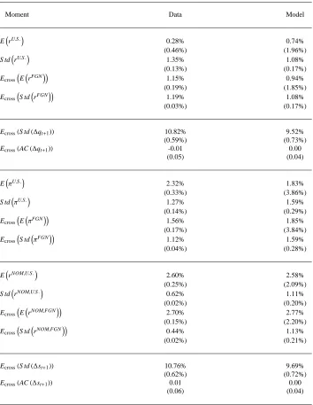
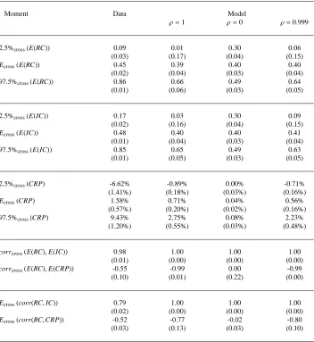
5.5. Model simulation
Finally, we assess the quantitative performance of our model and show that it can match key FX correlation moments, as well as the standard interest rate and exchange rate moments.
To illustrate the importance of unspanned FX correlation risk, we consider a nesting model; both our model and the Lustig, Roussanov and Verdelhan (2014) model are special cases of that nesting model. The law of motion of the local
pricing factor of country i, zi, in the nesting model is
∆zit+1 =λ(¯z−zit)−ξ
q zi
t
√
ρugt+1+ p1−ρuit+1, (21)