For Peer Review
Quantifying ice cliff evolution with multi-temporal point clouds on the debris-covered Khumbu Glacier, Nepal
Journal: Journal of Glaciology Manuscript ID JOG-17-0017.R3 Manuscript Type: Article
Date Submitted by the Author: n/a
Complete List of Authors: Watson, Cameron; University of Leeds, School of Geography and water@leeds
Quincey, Duncan; University of Leeds, School of Geography and water@leeds
Smith, Mark; University of Leeds, School of Geography and water@leeds Carrivick, Jonathan; University of Leeds, School of Geography and water@leeds
Rowan, Ann; University of Sheffield, Department of Geography James, Mike; Lancaster University, Lancaster Environment Centre
Keywords: Debris-covered glaciers, Remote sensing, Subglacial lakes, Glacial geomorphology, Glaciological instruments and methods
For Peer Review
Quantifying ice cliff evolution with multi-temporal point clouds
1
on the debris-covered Khumbu Glacier, Nepal
2
C. Scott Watson1, Duncan J. Quincey1, Mark W. Smith1, Jonathan L. Carrivick1, Ann V. 3
Rowan2,Mike James3 4
1. School of Geography and water@leeds, University of Leeds, Leeds, LS2 9JT, UK 5
2. Department of Geography, University of Sheffield, Sheffield, S10 2TN, UK 6
3. Lancaster Environment Centre, Lancaster University, Lancaster, LA1 4YQ, U.K. 7
Correspondence to: C. S. Watson ([email protected]) 8
ABSTRACT
9
Measurements of glacier ice cliff evolution are sparse, but where they do exist, they indicate 10
that such areas of exposed ice contribute a disproportionate amount of melt to the glacier 11
ablation budget. We used Structure from Motion (SfM) photogrammetry with Multi-View 12
Stereo (MVS) to derive 3D point clouds for nine ice cliffs on Khumbu Glacier, Nepal (in 13
November 2015, May 2016 and October 2016). By differencing these clouds, we could 14
quantify the magnitude, seasonality, and spatial variability of ice cliff retreat. Mean retreat 15
rates of 0.30 to 1.49 cm d-1 were observed during the winter interval (November 2015 to May 16
2016) and 0.74 to 5.18 cm d-1 were observed during the summer (May 2016 to October 17
2016). Four ice cliffs, which all featured supraglacial ponds, persisted over the full study 18
period. In contrast, ice cliffs without a pond or with a steep back-slope degraded over the 19
same period. The rate of thermo-erosional undercutting was over double that of subaerial 20
retreat. Overall, 3D topographic differencing allowed an improved process-based 21
understanding of cliff evolution and cliff−pond coupling, which will become increasingly 22
important for monitoring and modelling the evolution of thinning debris-covered glaciers. 23
1.
INTRODUCTION
24
In coming decades, ongoing mass loss from Himalayan glaciers and changing runoff trends 25
will affect the water resources of over a billion people in, including those who require it for 26
agricultural, energy production, and domestic usage (Immerzeel and others, 2009; Immerzeel 27
and others, 2010; Lutz and others, 2014; Mukherji and others, 2015; Shea and Immerzeel, 28
2016). A negative mass balance regime prevails across glaciers in the central and eastern 29
Himalaya (Bolch and others, 2011; Fujita and Nuimura, 2011; Benn and others, 2012; Kääb 30
and others, 2012; Kääb and others, 2015; King and others, 2017), which are widely 31
recognised to be out of equilibrium with current climate (Yang and others, 2006; Shrestha 32
and Aryal, 2011; Salerno and others, 2015). Deglaciation is leading to the development of 33
large proglacial lakes, which may expand rapidly through ice cliff calving (Bolch and others, 34
2008; Benn and others, 2012; Thompson and others, 2012; Thakuri and others, 2016), and 35
pose potential glacial lake outburst flood hazards (e.g. Carrivick and Tweed, 2013; Carrivick 36
and Tweed, 2016; Rounce and others, 2016; Rounce and others, 2017). 37
Debris-covered glaciers have a hummocky, pitted surface, caused by variable melt 38
rates under different debris thicknesses, and include extensive coverage of ice cliffs and 39
supraglacial ponds (Hambrey and others, 2008; Thompson and others, 2016; Watson and 40
others, 2016; Watson and others, 2017). Studies using Digital Elevation Model (DEM) 41
differencing to quantify elevation change over debris-covered tongues have revealed an 42
association between glacier surface lowering and the presence of ice cliffs and supraglacial 43
ponds (Immerzeel and others, 2014; Pellicciotti and others, 2015; Ragettli and others, 2016; 44
Thompson and others, 2016), confirming historical ice cliff observations (e.g. Inoue and 45
For Peer Review
However, raster-based DEMs generally give a poor representation of steep slopes or steeply-1
sloping topography (Kolecka, 2012) and their differencing incorporates a mixed signal 2
containing surface elevation change related to debris cover, ice cliff dynamics, supraglacial 3
ponds, and glacier emergence velocity (Vincent and others, 2016). 4
Models of glacier evolution do not consider pond dynamics or ice cliff dynamics 5
explicitly, because this requires an understanding of their spatio-temporal distribution (e.g. 6
Sakai and others, 2002; Watson and others, 2017), energy balance modelling of the ice cliff 7
surface (e.g. Reid and Brock, 2014; Steiner and others, 2015; Buri and others, 2016b; Buri 8
and others, 2016a), and cliff-scale observations of retreat rates (e.g. Brun and others, 2016). 9
Several studies have exploited topographic models derived from unmanned aerial vehicle 10
surveys of Lirung Glacier in the Langtang region of Nepal, to make substantial progress 11
towards understanding ice cliff dynamics (Immerzeel and others, 2014; Steiner and others, 12
2015; Brun and others, 2016; Buri and others, 2016b; Buri and others, 2016a; Miles and 13
others, 2016a). However, techniques to perform direct comparisons of multi-temporal point 14
clouds without simplification have yet to be exploited. 15
In this study, we explore ice cliff evolution using multi-temporal point clouds 16
obtained on Khumbu Glacier, Nepal. Specifically we: (1) quantify the retreat of ice cliffs for 17
pre-monsoon and monsoon time periods; (2) compare the spatial variation in retreat across 18
ice cliff faces; and (3) assess the change in ice cliff morphology through time in relation to 19
local topography and the presence of supraglacial ponds. 20
2.
STUDY SITE
21
Field data were obtained on Khumbu Glacier in the Everest region of Nepal during three field 22
campaigns (post-monsoon November 2015, pre-monsoon May 2016, and late-monsoon 23
October 2016). The November 2015 to May 2016 and May 2016 to October 2016 survey 24
intervals are referred to as ‘winter’ and ‘summer’ respectively. The Indian summer monsoon 25
spans the months of June to mid-October (Bollasina and others, 2002; Bonasoni and others, 26
2008) and is when ~80% of annual precipitation falls (Wagnon and others, 2013). 27
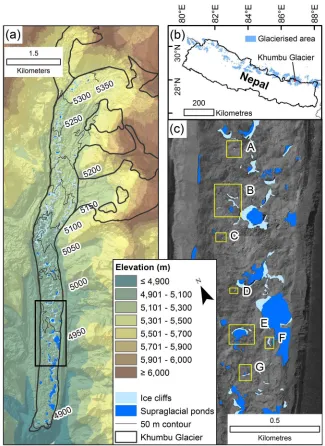
Khumbu Glacier is ~17 km long, of which the lower 10 km is debris covered (Fig. 1) 28
and the lower ~4 km is essentially stagnant (Quincey and others, 2009). Supraglacial debris 29
thickness is >2 m in this stagnating region and decreases up-glacier (Nakawo and others, 30
1986; Rowan and others, 2015). However, the thickness of the debris layer is locally 31
heterogeneous owing to the pitted surface and the presence of ice cliffs and supraglacial 32
ponds. We studied nine ice cliffs on the lower debris-covered glacier (Fig. 1), which is a 33
region of particular interest since supraglacial ponds have begun to coalesce here over the 34
past five years (Watson and others, 2016), and a large glacial lake is expected to form (Naito 35
and others, 2000; Bolch and others, 2011; Haritashya and others, 2015). 36
“Fig. 1 near here” 37
3.
DATA AND METHODS
38
3.1
Data collection
39
Terrestrial photographic surveys of nine ice cliffs were carried out during the three 40
field campaigns. Our study cliffs represented approximately 2% of the total ice cliff extent on 41
Khumbu Glacier, based on the top-edge cliff delineation of Watson and others (2017). We 42
sought to survey cliffs that were broadly representative of the range of cliffs found on 43
Khumbu Glacier, with and without supraglacial ponds, of variable aspect, and of variable 44
size, noting the terrestrial survey constraints that precluded surveys of very large cliffs. Four 45
of our nine study cliffs had a supraglacial pond present during the initial survey and the mean 46
length of ice cliffs was 57 m. This compares to the observation that on Khumbu Glacier 47% 47
For Peer Review
(Watson and others, 2017). We note from Watson and others (2017) that cliffs 20−40 m in 1
length were most common, but that some cliffs exceeded 200 m in length. 2
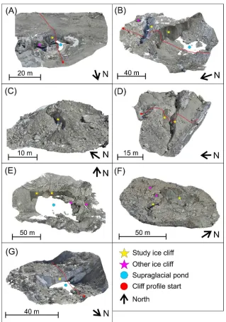
Two out of the seven individual study sites (Fig. 1) included both northerly- and southerly-3
facing cliff faces. These southerly-facing cliffs are labelled ‘-SF’ hereafter. Within the first 4
two field campaigns, surveys were conducted at intervals of 7–11 days at cliffs C, D, E and F, 5
which are referred to as ‘weekly’ surveys. ‘Seasonal’ surveys refer to those between field 6
campaigns. Each survey typically took <1 hour and 122–564 photos were taken of each ice 7
cliff with a highly convergent geometry (Fig. 2a) using a Panasonic DMC-TZ60 18.1 8
megapixel digital camera. In order to capture the surrounding topography, each photo was 9
taken from a different position but was not necessarily orientated towards the ice cliff. High-10
contrast temporary ground control points (GCPs) (number of GCPs (n) = 6–15) were 11
distributed around each ice cliff to encompass the survey area extents and surveyed using a 12
Leica GS10 global navigation satellite system (GNSS). Each GCP was occupied in static 13
mode for ~5 minutes. A base station was located on the lateral moraine of the glacier <2 km 14
from our survey sites for the duration of each field campaign and was set to record each day. 15
“Fig. 2 near here” 16
3.2 Post-processing 17
Our GNSS base station data were post-processed against the Syangboche permanent station 18
(27.8142 N, 86.7125 E) located ~20 km from our field site using Global Positioning System 19
(GPS) and GLObal NAvigation Satellite System (GLONASS) satellites. Our field GCPs were 20
then adjusted with reference to the field base station data following a relative carrier phase 21
positioning strategy. The mean 3D positional uncertainty was 3.9 mm across all our GCPs (n 22
= 281). 23
Photographs were input into Agisoft PhotoScan 1.2.3 to derive 3D point clouds of the 24
ice cliff topography following a Structure-from-Motion with Multiview Stereo (SfM-MVS) 25
workflow (e.g. James and Robson, 2012; Westoby and others, 2012; Smith and others, 2015). 26
First, photographs were aligned to produce a sparse point cloud by matching coincident 27
features. This stage also estimated internal camera lens distortion parameters and scene 28
geometry using a bundle adjustment with high redundancy, owing to large overlapping 29
photographic datasets (Westoby and others, 2012). Only points with a reprojection error of 30
<0.6 were retained and clear outliers (e.g. areas of shadow under overhanging cliffs) were 31
removed manually. Second, GCPs were identified in each photograph to georeference the 32
sparse cloud. GCP placement accuracy was <10 mm (e.g. Fig. 2b). Uncertainties from GCP 33
placement and the post-processed coordinates were used as weights to optimise the point 34
cloud georeferencing to minimise root-mean-square error (RMSE) (Javernick and others, 35
2014; Stumpf and others, 2015; Smith and others, 2016; Westoby and others, 2016). Third, a 36
dense point cloud was produced using PhotoScan’s multiview stereo (MVS) algorithm (Fig. 37
3). The dense cloud was subsequently edited to remove points that were not on solid surfaces 38
(e.g. on supraglacial ponds) and clear outliers. All PhotoScan’s processes were run on high 39
quality settings. Georeferencing uncertainty in the final point clouds was <0.035 m (RMSE; 40
Table 1). The final point clouds were sub-sampled using an octree filter in CloudCompare to 41
unify point density across the surveys for each individual ice cliff. Subsequent point cloud 42
densities ranged between 2,185–14,581 points per m2. 43
“Table 1. near here” 44
“Fig. 3 near here” 45
3.3
Ice cliff displacement
46
3.3.1 Ice cliff surveys between field campaigns 47
The study cliffs were located down-glacier of the expected active−inactive ice transition on 48
For Peer Review
m a-1) were observed in this region from dGPS surveys of tagged boulders (Supplementary 1
Fig. 1). Therefore, to correct for ice cliff displacement between field campaigns (November 2
2015 to May 2016 and May 2016 to Oct 2016) we co-registered point clouds using image 3
features that could be identified in multiple surveys (e.g. identifiable marks on boulders). For 4
each survey, the coordinates were derived for these features (as ‘Markers’ in PhotoScan), 5
enabling a transform (2D translation-rotation) to be calculated to co-register the later model 6
with the earlier one. The RMSE between these co-registered features are reported in Table 1, 7
and were used as the total error (ET) in subsequent point cloud differencing. Co-registration
8
errors were subject to sub-debris melt over each differencing period; however, thick debris 9
cover (1−>2 m) (Nakawo and others, 1986) and low sub-debris melt rates of 0.0015 m d-1 10
(Inoue and Yoshida, 1980) over our study area minimised these errors. Glacier emergence 11
velocity could not be calculated for this study; however, this is expected to be low for the 12
slow-moving and gently-sloping debris-covered study area (Nuimura and others, 2012). 13
3.3.2 Ice cliff surveys within field campaigns 14
To account for cliff displacement between repeat surveys within each field campaign (e.g. 15
Cliff C 03/11/2015 and 10/11/2015), we take the mean daily displacement of the respective 16
cliff between field campaigns (e.g. 0.0023 m d-1) and multiply this by the time-separation of 17
the repeat models (e.g. seven days). The resulting shift (e.g. 0.0161 m) was treated as an 18
additional uncertainty in addition to the respective georeferencing errors. We did not shift 19
these models as described in section 3.3.1, since the expected displacement was <0.04 m for 20
all ice cliffs, which was similar to the uncertainty in identifying coincident features in each 21
model. 22
To calculate the total error (ET) for each cliff model comparison within a field
23
campaign, the individual errors were propagated using (1): 24
1 = + +
25
Where GEC1and GEC2are the georeferencing RMS errors associated with clouds C1 and C2,
26
and DEC1-C2is the displacement error between clouds C1 and C2.
27
3.4
Point cloud characteristics and differencing
28
The mean slope and aspect of ice cliffs were calculated in CloudCompare using the dip 29
direction and angle tool. The aspect of overhanging cliff sections required correction through 30
180°. The area of cliffs was calculated by fitting a mesh to each point cloud using the Poisson 31
Surface Reconstruction tool in CloudCompare (Kazhdan and Hoppe, 2013). 32
Cloud-to-cloud differencing was carried out in the open source CloudCompare software 33
using the Multiscale Model to Model Cloud Comparison (M3C2) method (e.g. Barnhart and 34
Crosby 2013; Lague and others, 2013; Gomez-Gutierrez and others, 2015; Stumpf and others, 35
2015; Westoby and others, 2016). M3C2 was created by Lague and others (2013) to quantify 36
the 3D distance between two point clouds along the normal surface direction and provide a 37
95% confidence interval based on the point cloud roughness and co-registration uncertainty. 38
The method is therefore ideally suited to quantifying statistically significant ice cliff 39
evolution where the geometry changes in 3D, and is robust to changes in point density and 40
point cloud noise (Barnhart and Crosby, 2013; Lague and others, 2013). 41
For point clouds derived from photogrammetric techniques, uncertainty is spatially 42
variable but highly correlated locally, since points in close proximity to one another are 43
derived from the same images (James and others, 2017). Thus, although point-cloud 44
roughness could represent a component of the measurement precision required to derive 45
confidence intervals, it would not include broader photogrammetric contributions. In order to 46
visualise spatially variable photogrammetric and georeferencing precision, we derived 3D 47
For Peer Review
(Supplementary Fig. 2). Repeated bundle adjustments implemented in PhotoScan (4000 1
Monte Carlo iterations) were applied to the sparse point cloud of each ice cliff using GCP and 2
tie point uncertainties. Point precision estimates were then interpolated onto a 1 m raster grid 3
in sfm_georef v3.0 (James and Robson, 2012; James and others, 2017). Large uncertainties 4
were apparent at the survey edges (e.g. Cliff A, C, D, E), and around supraglacial ponds (e.g. 5
Cliff E) due to poor photograph coverage. In contrast, the mean precision estimates ranged 6
from 7−38 mm and were uniform across individual cliff faces. Hence, given the large 7
magnitudes of the measured ice cliff changes, the M3C2-PM (Precision Maps) variant based 8
on photogrammetry-derived precision maps was not required and the native M3C2 algorithm, 9
implemented in CloudCompare, was used throughout. 10
M3C2 requires two user-defined parameters: (1) the normal scale D, which is used to 11
calculate surface normals for each point and is dependent upon surface roughness and point 12
cloud geometry, and (2) the projection scale d over which the cloud-to-cloud distance 13
calculation is averaged, which should be large enough to average a minimum of 30 points 14
(Lague and others, 2013). We estimated the normal scale D for each point cloud following a 15
trial-and-error approach similar that of Westoby and others (2016), to reduce the estimated 16
normal error, Enorm (%), through refinement of a rescaled measure of the normal scale n(i):
17
2 =
n(i) is the normal scale D divided by the roughness σ measured at the same scale around i. 18
Where n(i) falls in the range 20–25, Enorm <2% (Lague and others, 2013). In this study,
19
normal scales D ranged from 1.5−8 m and the projection scale d was fixed at 0.3 m. The 20
Level of Detection (LoD) threshold for a 95% confidence level is given by: 21
3 % = ±1.96 !"#$
%
&# +
"%$%
&% + '()* 22
where σ1andσ2represent the roughness of each point in sub-clouds of diameter d and size n1
23
and n2, and reg is the cloud-to-cloud co-registration error, for which ET is substituted. The
24
error is assumed to be isotropic and spatially uniform across the dataset (Lague and others, 25
2013). 26
Distance calculations were masked to exclude points where the change was lower than the 27
Level of Detection (LoD) threshold and were clipped to individual ice cliff faces. Ice cliff 28
retreat rates were divided by respective survey intervals to derive daily retreat rates. Since 29
cliffs often exhibited large changes in geometry between surveys, some cliff normals at time 30
one intersected debris cover at time two. The total retreat of the cliff face was therefore 31
reported, in addition to cliff-to-cliff retreat (i.e. where cliff normals at time one intersected a 32
cliff at time two). 33
3.5
Other data
34
Volumetric loss due to ice cliff retreat was estimated from DEM differencing using point 35
clouds gridded at 0.5 m. Cliff retreat rates were also calculated using these volumetric 36
changes for comparison with M3C2 retreat rates, by dividing the volume loss over the 37
respective time period by the cliff area. The zone of ice cliff retreat was defined as the area 38
connected by cliff outlines at respective time periods. Where a cliff partially or completely 39
degraded and hence was not represented by an outline at time two, the zone of cliff retreat 40
was estimated using M3C2 distance measurements (representing spatially variable ice cliff 41
retreat) from the cliff at time one. These distance measurements were used to define a 42
variable-width buffer in ArcGIS to delineate the maximum extent of ice cliff retreat. 43
The drainage of the supraglacial pond adjacent to Cliff E provided an opportunity to 44
For Peer Review
2016, with the assumption that subaqueous basal melt and debris inputs to the basin were 1
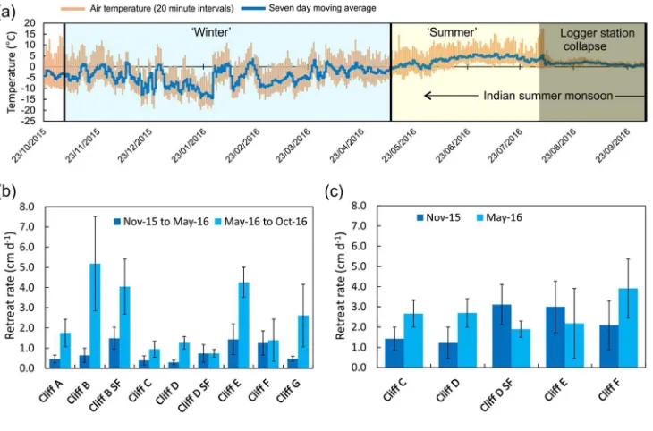
minimal. Additionally, air temperature at 1 m above the surface was recorded at 20 minute 2
intervals on Khumbu Glacier using a Solinst Barologger Edge, which was sited behind Cliff 3
G. Measurements were recorded from October 2015 to October 2016; however, the station 4
collapsed in August 2016 due to the retreat of Cliff G. The logger was found in an air pocket 5
buried by debris, hence data shown after this collapse revealed a subdued diurnal temperature 6
cycle. 7
4.
RESULTS
8
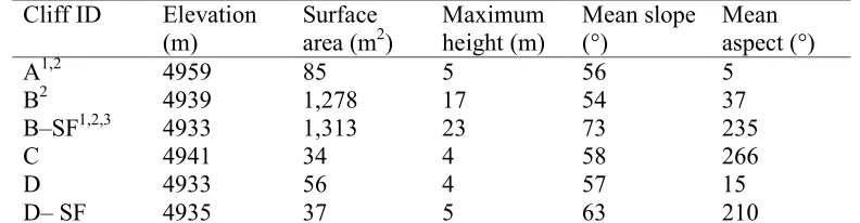
4.1 Summary ice cliff characteristics 9
Ice cliffs: ranged from 4 to 23 m in height; were all within a 43 m elevation range; had mean 10
slopes of 50 to 73°; and were of variable aspect, with both northerly- and southerly-facing 11
cliffs represented (Fig. 4, Table 2). Of the four cliffs with a supraglacial pond present in 12
November 2015, only Cliff B had a pond remaining in October 2016. Overall, four study 13
cliffs persisted throughout the study period and the other five were buried under debris 14
between May 2016 and October 2016 (Fig. 4c). 15
“Table 2. near here” 16
The mean slope, maximum cliff height, cliff area, and mean cliff aspect were 17
evaluated across our study period (Fig. 4). Southerly-facing cliffs generally featured higher 18
mean slopes, and the greatest changes in cliff slope were observed on southerly-facing cliffs 19
B-SF and E (Fig. 4a). Maximum cliff height reduced for all cliffs over the study period, 20
although this change was generally small for those cliffs that persisted through the study. 21
Cliff E, which lost ~5 m in height over summer (Fig. 4b), was an exception. Notably, 22
persistent cliffs had a starting height greater than 10 m; however, we note that Cliff F 23
decayed, despite a starting height greater than 10 m. With the exception of Cliff B-SF which 24
increased in area, all other cliffs declined in area over the study; however, the rate of this area 25
loss varied from cliff to cliff. Of the four cliffs persisting over the study, two were southerly-26
facing and two were northerly-facing and all had a supraglacial pond present for part of the 27
study period (Table 2). However, pond dynamics between the observation dates were 28
unknown. The largest changes in cliff aspect were for cliffs C and D-SF, which became 29
increasingly northerly and westerly orientated by 25° and 23° respectively (Fig. 4d). 30
“Fig. 4 near here” 31
4.2 Ice cliff retreat 32
With the exception of Cliff D-SF, cliff retreat rates were higher over summer than the 33
preceding winter, which corresponds with consistently higher air temperatures during 34
summer (Fig. 5, Table 3). Mean winter temperatures were generally below 0°C, whereas 35
summer temperatures were generally above 0°C, although several discrete periods of positive 36
air temperature also occurred in winter. Similarly, volumetric losses due to cliff retreat were 37
generally higher during summer, although they were small where cliffs degraded (e.g. D-SF, 38
Table 3). Notably, the M3C2- and DEM-based retreat rates were comparable for most cliffs. 39
The highest mean retreat rate occurred at Cliff B and B-SF during summer, although this was 40
a combination of subaerial retreat and a large-scale cliff collapse involving a section of the 41
cliff ~30 m in length. Excluding this cliff face, the highest mean retreat rates observed and 42
the largest seasonal differences in retreat rates were from ice cliffs with an adjacent 43
supraglacial pond including cliffs A (1.75 cm d-1), E (4.26 cm d-1) and G (2.62 cm d-1) (Fig. 44
5b). The retreat rates for weekly surveys were generally higher than seasonal retreat rates, 45
with the exception of Cliff E (Fig. 5). Retreat rates for cliffs that degraded over the study 46
period (A, C, D, D-SF, and F) included a transition to sub-debris melt during the summer, 47
For Peer Review
cliffs. Similarly, where cliffs partially degraded between survey intervals, the cliff-to-cliff 1
retreat was generally greater than the total retreat rates, which included areas of cliff-to-debris 2
transition (Table 3). Here, retreat rates attributed only to persistent areas of cliff ranged from 3
0.36−1.68 cm d-1 (winter), and 3.84−5.85 cm d-1 (summer). 4
“Fig. 5 near here” 5
“Table 3 near here” 6
Across individual cliff faces, the observed retreat was related to the presence of supraglacial 7
ponds, englacial conduits (expressed as an opening within or below ice cliff faces), cliff 8
aspect, cliff slope, and the formation of runnels (Fig. 6). Mean winter ice cliff retreat showed 9
a clear relationship with aspect and peaked at a south easterly aspect of 155º, although this 10
was not the case during summer (Fig. 6h). Maximum retreat rates (10.65 cm d-1) were 11
observed at cliffs B and B-SF (Fig. 6b) where a notable calving event occurred in the 12
summer. This was followed by northerly-facing Cliff G in association with a supraglacial 13
pond, with maximum retreat rates of 6.18 cm d-1 in the zone of thermal undercutting (Fig. 14
6g). The surface of this pond was frozen between the November 2015 and May 2016 surveys 15
and the pond had drained by October 2016. 16
Runnels were locations of locally differential retreat on the north-facing cliffs B and 17
G during winter (Fig. 6b, g) and these cliffs also had the lowest mean initial slopes of 54° and 18
50° respectively (Table 2). During winter, the relative increase in retreat at Cliff G at 19
locations of runnels was ~0.12−0.24 cm d-1 (Fig. 6g). However, the presence of runnels was 20
localised and, when considering the whole cliff, the rate of runnel retreat (~0.47−0.58 cm d-1) 21
was otherwise comparable to the mean retreat rate during winter (0.47 cm d-1). Evidence of a 22
vertical retreat gradient was apparent on several cliffs during winter (e.g. Fig. 6c, d, f), and 23
was similar during summer, other than where thermal undercutting was apparent (e.g. Cliff 24
G). Cliff B-SF featured the most apparent aspect-related control on retreat during winter with 25
westerly facing ice melting at the slowest rate (~0.84 cm d-1) compared to southerly faces 26
(~2.62 cm d-1, Fig. 6b). Cliff A featured an englacial conduit large enough to enable crouched 27
access into a void behind the cliff face, which was the area of greatest retreat for this cliff 28
(~4 cm d-1 during summer) as the void likely became exposed and degraded (Fig. 6a). 29
“Fig. 6 near here” 30
4.3 Ice cliff evolutionary traits 31
2D profiles through selected ice cliffs revealed different characteristics of retreat, including 32
ice cliff burial under debris, ice cliff collapse, and undercutting by adjacent supraglacial 33
ponds (Fig. 7). Cliff A maintained a similar slope during its retreat over winter, although 34
during summer the slope angle decreased to ~35°, which led to burial under debris (Fig. 7a). 35
There was a small supraglacial pond shallower than 1 m adjacent to Cliff A in the November 36
2015 and May 2016 surveys, and an associated undercut notch. The pond drained prior to the 37
October 2016 survey, and the steep cliff back-slope led to a relaxation of the cliff slope and 38
hence degradation of Cliff A by October 2016. 39
The profile through Cliff B revealed greater retreat on the southerly face through 40
winter, compared to the northerly face (Fig. 7b). A section of Cliff B collapsed prior to the 41
final survey in October 16, suggesting that the undercut notch caused the cliff to collapse in a 42
northerly direction. The supraglacial pond in contact with Cliff B-SF expanded throughout 43
the study and was in contact with the southerly face (although not at the 2D profile shown), 44
which exposed a new ice cliff face and caused an increase in cliff area (Fig. 4c). A 45
supraglacial pond was present at the northerly-facing Cliff B in May 2016; however, the 46
For Peer Review
The two opposing faces of Cliff D and D-SF both became buried over the study (Fig. 1
7c). The southerly-facing cliff retreated faster than the northerly face during winter; however, 2
the steep back-slope and small area of this southerly face limited the retreat during summer. 3
Debris infill was apparent in the May 2016 profile, caused by the retreat of the southerly face, 4
which had an inwardly sloping cliff top. 5
Cliff E featured a supraglacial pond over 9.95 m deep, which drained over the 6
summer. There was evidence of deepening towards the cliff faces at profiles 1 and 2 and 7
thermal undercutting of both cliff faces (Fig. 8c, d). The pond at Cliff G also drained over 8
the summer and was also associated with an undercut notch. Cliff G had a gentle back-slope 9
and maintained a similar slope (50−54°) during retreat (Fig. 7d). The gentle back-slope of 10
Cliff G allowed continued retreat, in contrast to cliffs A and D where a steep back-slope lead 11
to cliff degradation. 12
“Fig. 7 near here” 13
“Fig. 8 near here” 14
5.
DISCUSSION
15
5.1 Multi-temporal ice cliff surveys 16
In this study we have presented the first application of 3D point cloud differencing to multi-17
temporal topographic surveys of ice cliffs, revealing evolutionary traits for a variety of ice 18
cliffs present on the lower ablation area of Khumbu Glacier. This method has specific 19
advantages for quantifying the importance of ice cliff retreat and the cliff−pond interaction 20
when compared to previous approaches. First, the retreat attributed to ice cliffs is calculated 21
along the normal direction of the cliff face, thereby minimising the conflation of topographic 22
change from debris cover, ice cliffs and supraglacial ponds, that exists in vertical DEM 23
differencing (e.g. Thompson and others, 2016). However, where a cliff decays between two 24
survey dates, retreat calculations include topographic change related to processes in addition 25
to cliff retreat such as sub-debris melt, hence short survey intervals are preferable. M3C2 26
allows quantification of the variability of retreat across a cliff face, for example in relation to 27
slope and aspect (Buri and others, 2016a), the presence of runnels (Watson and others, 28
2017), and supraglacial ponds (Miles and others, 2016a). Second, the mechanism controlling 29
topographic change can be evaluated in three dimensions, revealing the role of ice cliff back-30
slope in ice cliff persistence, and thermo-erosional undercutting by supraglacial ponds. 31
5.2 Ice cliff retreat 32
Observations of ice cliff retreat have previously been obtained from point ablation stake 33
measurements or using static markers on the back-slopes of ice cliffs (e.g. Inoue and 34
Yoshida, 1980; Sakai and others, 1998; Purdie and Fitzharris, 1999; Sakai and others, 2002; 35
Benn and others, 2001; Han and others, 2010; Reid and Brock, 2014; Steiner and others, 36
2015). Use of ablation stakes restricts assessment of the spatial variation in retreat across an 37
ice cliff face, since stake placements are likely to be aligned vertically down the cliff face and 38
biased towards areas of comparatively safer access. In comparison, Brun and others (2016) 39
used multi-temporal fine-resolution topographic surveys to estimate the volumetric mass loss 40
and mean retreat rates from five ice cliffs on the debris-covered Lirung Glacier. Their study 41
cliffs were generally larger (maximum face size of 6441 m2 compared to 1313 m2 in this 42
study), and at ~800 m lower elevation. 43
5.2.1 Ice cliff retreat through time 44
Four of nine ice cliffs, which all had a maximum height >10 m (Fig. 4b) and featured an 45
adjacent supraglacial pond (Table 2), persisted over one year in this study. In contrast, all 46
study cliffs of Brun and others (2016) persisted over one year and were all ≥9 m high. Mean 47
For Peer Review
cm d-1 (summer) and were comparable to those of Brun and others (2016), 0.70 to 1.20 cm d-1 1
(winter) and 2.2 to 4.5 cm d-1 (summer), despite the higher elevation and smaller size of our 2
study cliffs. In our study, ice cliff retreat rates were generally higher during summer and for 3
southerly-facing ice cliffs, and summer featured the largest variability in retreat rates amongst 4
cliffs (Fig. 5b, c). Lower retreat rates during winter correspond with cooler air temperatures 5
(Fig. 5a). Higher retreat rates during the November 2015 weekly surveys compared to 6
respective seasonal surveys, reflected warmer temperatures before winter. Similarly, the May 7
2016 surveys generally had higher retreat rates than the May 2016 to October 2016 surveys 8
(Fig. 5b, c). For cliffs C, D and F, this likely reflects cliff degradation before October 2016 9
and hence a transition from cliff retreat to sub-debris melt for part of the survey interval. The 10
unknown date of cliff degradation is a limitation to assessing mass loss relating only to ice 11
cliff retreat. However, the retreat rates for cliffs that partially degraded between surveys can 12
be quantified by considering the total cliff retreat, which includes areas where the cliff 13
degraded, and the cliff-to-cliff retreat, where cliff normals at time one intersect a cliff at time 14
two (Table 3, Supplementary Table 1). The former is representative of the total cliff 15
evolution, which includes areas of ice cliff degrading and becoming buried by debris, 16
whereas the latter is representative of the retreat rates for persisting areas of cliff. 17
Cliff B suffered a partial collapse of a ~30 m segment during summer, causing high mass 18
loss due to the effect of this calving event (Fig. 5b, Table 3). Similarly high retreat rates May 19
2016 to October 2016 were observed at cliffs E and G, which both featured supraglacial 20
ponds becoming active (i.e. thawed) during summer. The high variation in retreat rates over 21
summer suggests that more frequent monitoring would be beneficial to assess cliff dynamics 22
such as burial under debris and the interaction with seasonally expanding supraglacial ponds. 23
5.2.2 Cliff face variation in retreat 24
Visualising the spatial distribution of retreat across individual cliff faces revealed vertical and 25
lateral gradients, and increased retreat attributed to supraglacial ponds during summer (Fig. 26
6). The influence of cliff aspect is apparent on Cliff B-SF, where a southerly face retreated 27
1.78 cm d-1 faster than an adjacent westerly face (Fig. 6b). Both the north-facing cliffs B and 28
G displayed evidence of locally enhanced retreat attributed to the presence of vertical runnels 29
observed during the winter surveys (Fig. 6b, g). Runnels were also observed by Watson and 30
others (2017) on other ice cliffs on Khumbu Glacier. The low solar radiation receipt on 31
northerly-facing cliffs during winter may mean that meltwater generated at the less shaded 32
cliff top from sub-debris melt and from melt on the cliff face is able to incise runnels faster 33
than the background rate of cliff retreat. In contrast, during summer the higher magnitude of 34
retreat likely masks this influence of micro-scale cliff topography (Fig. 6), although the 35
runnels may persist. Runnels also act as preferential pathways for debris slumping from the 36
cliff top and differential retreat may also occur in response to albedo variations across the 37
cliff face. The morphology of the cliff face, including runnel development and self-shading, 38
is therefore likely to locally influence retreat rates as evidenced in this study, but should be 39
explored further with additional 3D surveys in order to assess their importance seasonally, 40
and at a glacier scale. 41
Cliff tops exhibited the highest retreat rates in several cases (e.g. Fig. 6c, d, f), which was 42
also observed in the modelled retreat rates at two ice cliffs by Buri et al. (2016b). Cliff G also 43
displayed a vertical gradient during the summer; however, this was locally reversed in the 44
area undercut by a supraglacial pond (Fig. 6g). 45
5.2.3 The influence of aspect
46
Several studies have observed a prevalence of northerly-facing ice cliffs on debris-covered 47
glaciers in the Northern Hemisphere, suggesting that solar radiation receipt plays a key role 48
in controlling ice cliff development (Sakai and others, 2002; Kraaijenbrink and others, 2016b; 49
For Peer Review
expected to decay quickly after formation due to high solar radiation receipt, whereas 1
northerly-facing cliffs are more persistent (Sakai and others, 2002). Slope relaxation was 2
apparent on southerly-facing cliffs B-SF and E, which decreased by 14 and 13° respectively; 3
however, both of these cliffs persisted throughout the study period. 4
We observed highest ice cliff retreat rates on ice cliffs with a southeasterly aspect (155º) 5
(Fig. 6h), although this trend was only apparent during winter. Also on Khumbu Glacier, 6
Inoue and Yoshida (1980) revealed maximum ice cliff retreat at an aspect of ~190º. Cliff 7
aspect likely has a stronger influence over cliff retreat in the winter due to the low solar angle 8
and cliff self-shading (e.g. Steiner and others, 2015). Additionally, direct solar radiation 9
receipt is reduced during the summer monsoon due to the prevalence of cloud cover 10
(Supplementary Fig. 4). Therefore at this time, diffuse radiation, air temperature, and local 11
ice cliff characteristics such as the presence of a supraglacial pond were likely stronger 12
controls on ice cliff retreat than the cliff aspect. 13
14
5.3 Local controls on ice cliff evolution 15
The back-slope of individual ice cliffs influences their longevity, since there is a finite 16
volume of ice for the cliff to retreat into unless accompanied by simultaneous downwasting 17
of a supraglacial pond. In our study, slope relaxation and cliff degradation (Fig. 4a, 7a and c) 18
were observed on both northerly- and southerly-facing ice cliffs. This contrasts with the 19
observations of Sakai and others (2002) where slope relaxation was a trait of southerly-facing 20
ice cliffs, highlighting the importance of local topography and cliff characteristics, which 21
determine the longevity of individual ice cliffs over an ablation season. 22
Several studies have observed strong spatial coincidence of ice cliffs and supraglacial 23
ponds (Thompson and others, 2016; Watson and others, 2017) and notable subaqueous melt 24
rates (Sakai and others, 2009; Miles and others, 2016a). The potential importance of ponds 25
for enhancing ice cliff retreat on Himalayan debris-covered glaciers is analogous to the 26
‘wandering lakes’ on Antarctic ice-cored moraines (e.g. Pickard, 1983). Thompson and 27
others (2016) observed that 75% of ice cliffs were associated with a supraglacial pond on the 28
Ngozumpa Glacier, and an average of 49% was observed by Watson and others (2017) across 29
14 glaciers in the Everest region of Nepal; however, these associations are likely to be 30
seasonally variable. Our study revealed greater retreat for ice cliffs associated with a 31
supraglacial pond, and mean retreat rates of pond-contact ice were estimated to be double that 32
of subaerial retreat at Cliff G. However, the pond at Cliff G drained prior to the final survey 33
such that the role of the pond could not be fully isolated from subaerial retreat. All persisting 34
ice cliffs featured a supraglacial pond during their lifespan. We suggest that undercut notches 35
allowed the cliff angle to be maintained during retreat, which promoted cliff persistence (e.g. 36
Fig 7d, 8d). Therefore our observations, in addition to strong association of cliffs and ponds 37
(e.g. Watson and others, 2017), suggest that supraglacial ponds are likely to play a key role in 38
ice cliff retreat and persistence at a glacier scale. However, quantifying subaqueous retreat 39
using point cloud differencing is hindered by submerged topography, and manual field 40
measurements (e.g. Rohl, 2006) are restricted by falling debris. Additionally, we cannot 41
comment on the spatial variation in the importance of ice cliff retreat, which likely decreases 42
with distance up-glacier using due to thinning debris cover (Thompson and others, 2016; 43
Watson and others, 2017). 44
5.4 Implications for mass loss at a glacier scale 45
The ice cliff retreat rates observed in this study support previously observed associations 46
between glacier surface lowering and the presence of ice cliffs and supraglacial ponds 47
(Immerzeel and others, 2014; Pellicciotti and others, 2015; Thompson and others, 2016; 48
Watson and others, 2017). Observed mean ice cliff retreat rates ranged from 0.30 (winter) to 49
For Peer Review
observed in a similar region of Khumbu Glacier by Inoue and Yoshida (1980). However, we 1
note that these rates are not directly comparable since our observations represent surface-2
normal retreat, whereas sub-debris melt represents vertical lowering. The rate of surface 3
lowering related to debris cover ranged from 0.03−0.31 cm d-1 on the nearby Ngozumpa 4
Glacier based on the DEM differencing of Thompson and others (2016). However, surface 5
lowering observed from DEM differencing is a function of sub-debris melt and emergence 6
velocity. The latter was not quantified by Thompson et al. (2016), or in this study, but was 7
shown to be +0.37 m w.e a-1 (water equivalent) on the debris-covered Changri Nup Glacier 8
(Vincent and others, 2016). 9
10
The volumetric loss at ice cliffs is variable and highlights the requirement to up-scale our 11
methodology to the glacier scale in order to capture the full size distribution of ice cliffs 12
present (Table 3). Additionally, knowledge of fine spatio-temporal dynamics of supraglacial 13
ponds is still limited, but reveals potentially large seasonal expansion and contraction of 14
ponds (e.g. Miles and others, 2016b; Watson and others, 2016). This restricts efforts to model 15
the ice cliff−pond interaction (Buri and others, 2016a), or to quantify subaqueous retreat with 16
multi-temporal point clouds. Nonetheless, our results suggest that undercut notches can 17
promote ice cliff persistence by maintaining the slope angle during retreat. However, this 18
requires further investigation at a glacier scale and over longer time periods, with particular 19
attention to the role of undercutting for promoting calving events.A SfM-MVS methodology 20
using time-lapse imagery is one such approach that could provide high temporal resolution. 21
5.4.1 Future work
22
M3C2 offers new opportunities to quantify 3D topographic change on debris-covered glaciers 23
and this could be used to explore debris redistribution and the formation of ice cliffs, which 24
are currently limiting factors in modelling efforts (Buri and others, 2016a). Similarly, using 25
point cloud data and M3C2 can address several problems related to fine spatio-temporal 26
resolution DEM differencing, including the conflation of several processes contributing to the 27
topographic change signal, including ice cliff retreat, sub-debris melt, and supraglacial pond 28
basal melt. Debris thickness estimated along the top edge of the cliff could be accounted for 29
when slumping into supraglacial ponds, which may otherwise be counted as mass loss in 30
DEM differencing. Comparisons of coincident measurements of 3D and 2D topographic 31
change would therefore be highly beneficial to fully quantify their limitations. Additionally, 32
the topographic change could be explored further with a greater dataset of ice cliff 33
observations, to quantify specific relationships between cliff retreat and variables such as 34
local slope, aspect, and pond presence. However, our dataset demonstrates that ice cliff 35
evolution is highly heterogeneous and that, when considering the dataset as a whole, the 36
relationship between cliff retreat and slope, aspect, and pond presence would be highly 37
complex. Moving forward, conceptualising ice cliff evolution requires both local 38
observations as presented in this study, and glacier scale multi-temporal ice cliff datasets (e.g. 39
Watson and others, 2017). 40
The M3C2 method is not without its own limitations since it is difficult to calculate 41
volumetric mass loss due to the variable alignment of surface normals; however, such 42
methods are likely to become available or can be developed independently for similar 43
applications (e.g. Brun and others, 2016). Non-uniform glacier surface displacement also 44
presents issues when co-registering multi-temporal point clouds; however, this is arguably 45
easier to achieve than using a DEM due to the availability of true-colour point data. However, 46
DEMs and corresponding orthophotos can also be used for this correction (e.g. Kraaijenbrink 47
and others, 2016a). Non-uniform glacier surface displacement is an important consideration if 48
investigating lower magnitude processes such as sub-debris melt, which also requires 49
quantification of glacier emergence velocity (Vincent and others, 2016). Emergence velocity 50
For Peer Review
and others, 2011); however, positive surface elevation change was observed in this study (e.g. 1
Fig. 6f), which was confirmed by independent dGPS boulder surveys (used in Supplementary 2
Fig. 1). Additionally, point cloud precision estimates based on rigorous photogrammetric 3
processing rather than surface roughness allow improved topographic change detection 4
(James and others, 2017). 5
6.
CONCLUSIONS
6
We have presented the first multi-temporal 3D analysis of ice cliff evolution using 3D point 7
cloud differencing, which was necessary to quantify the spatial heterogeneity of retreat across 8
individual cliff faces and their interaction with supraglacial ponds. Our results revealed the 9
importance of a gentle cliff back-slope to allow continued retreat, and the role of supraglacial 10
ponds in thermo-erosional undercutting, which maintains the cliff angle and delays burial 11
under debris. Mean ice cliff retreat rates observed in this study ranged from 0.30 to 1.49 cm 12
d-1 (winter), and 0.74 to 5.18 cm d-1 (summer). Additionally, the four ice cliffs persisting over 13
our one year study period were all influenced by supraglacial ponds, and pond-contact ice 14
was associated with a two-fold increase in retreat at Cliff G. Our findings add further 15
evidence to the role of ice cliffs as ‘hot-spots’ of mass loss on heavily debris-covered glaciers 16
and contribute to a previously sparse dataset of ice cliff observations, revealing local controls 17
on cliff retreat which can be used to validate emerging models of ice cliff evolution (Brun 18
and others, 2016; Buri and others, 2016a). 19
We observed an aspect-related control on ice cliff retreat during winter; however, 20
local ice cliff characteristics masked any cliff-scale aspect related control on retreat during 21
summer. We observed examples of northerly- and southerly-facing cliffs persisting, but also 22
examples of cliff burial under debris. The controlling factors for ice cliff persistence appeared 23
to be cliffs with a maximum height >10 m and with supraglacial pond influence. Nonetheless, 24
the prevalence of northerly-facing cliffs on debris-covered glaciers in the northern 25
hemisphere (Sakai and others, 2002; Brun and others, 2016; Watson and others, 2017) 26
suggests that over longer timescales (e.g. decadal) the persistence of northerly-facing cliffs is 27
greater in response to self-shading and supraglacial pond association. 28
M3C2 point cloud differencing was shown to be an effective tool to quantify the spatio-29
temporal magnitude of retreat across ice cliff faces, and to offer a new opportunity to validate 30
models of ice cliff evolution. It is also more practical than point-based ablation stake 31
measurements. M3C2 could be applied to glacier scale point clouds to enable surface 32
elevation change to be partitioned into surface-normal (ice cliff retreat) and vertical (sub-33
debris and subaqueous melt) components, and should be compared to the prevailing practice 34
of DEM differencing. These 3D point cloud data provide a much more realistic representation 35
of surface area compared to a planimetric DEM, and minimise the conflation of different 36
topographic change signals that are common to DEM differencing. 37
7.
ACKNOWLEDGEMENTS
38
C.S.W acknowledges support from the School of Geography at the University of Leeds, the 39
Mount Everest Foundation, the British Society for Geomorphology, the Royal Geographical 40
Society (with IBG), the Petzl Foundation, and water@leeds. The Natural Environment 41
Research Council Geophysical Equipment Facility is thanked for loaning Global Navigation 42
Satellite Systems receivers and technical assistance under loan numbers 1050, 1058, and 43
1065. Dhananjay Regmi and Himalayan Research Expeditions are thanked for fieldwork 44
support including research permit acquisition, and Mahesh Magar is thanked for invaluable 45
support during data collection. Patrick Wagnon is thanked for providing access to AWS data. 46
This AWS has been funded by the French Service d’Observation GLACIOCLIM, the French 47
National Research Agency (ANR) through ANR-13-SENV-0005-04/05-PRESHINE, and has 48
For Peer Review
LABX56). CloudCompare (version 2.8, 2016) is GPL software retrieved from 1
http://www.cloudcompare.org/. Pleiades images were supplied by Airbus Defence and Space 2
through a Category-1 agreement with the European Space Agency (ID Nr. 32600). We thank 3
two anonymous reviewers for thorough and constructive reviews. 4
REFERENCES
5
Barnhart, T. and Crosby, B. 2013. Comparing two methods of surface change detection on an 6
evolving thermokarst using high-temporal-frequency terrestrial laser scanning, 7
selawik river, Alaska. Remote Sensing. 5(6), pp.2813-2837. 8
Benn, D.I. Bolch, T. Hands, K. Gulley, J. Luckman, A. Nicholson, L.I. Quincey, D. 9
Thompson, S. Toumi, R. and Wiseman, S. 2012. Response of debris-covered glaciers 10
in the Mount Everest region to recent warming, and implications for outburst flood 11
hazards. Earth-Science Reviews. 114(1–2), pp.156-174. 12
Benn, D.I. Wiseman, S. and Hands, K.A. 2001. Growth and drainage of supraglacial lakes on 13
debris-mantled Ngozumpa Glacier, Khumbu Himal, Nepal. Journal of Glaciology. 14
47(159), pp.626-638. 15
Bolch, T. Buchroithner, M.F. Peters, J. Baessler, M. and Bajracharya, S. 2008. Identification 16
of glacier motion and potentially dangerous glacial lakes in the Mt. Everest 17
region/Nepal using spaceborne imagery. Nat. Hazards Earth Syst. Sci. 8(6), pp.1329-18
1340. 19
Bolch, T. Pieczonka, T. and Benn, D.I. 2011. Multi-decadal mass loss of glaciers in the 20
Everest area (Nepal Himalaya) derived from stereo imagery. The Cryosphere. 5(2), 21
pp.349-358. 22
Bollasina, M. Bertolani, L. and Tartari, G. 2002. Meteorological observations in the Khumbu 23
Valley, Nepal Himalayas. Bulletin of Glaciological Research. 19, pp.1-11. 24
Bonasoni, P. Laj, P. Angelini, F. Arduini, J. Bonafè, U. Calzolari, F. Cristofanelli, P. 25
Decesari, S. Facchini, M.C. Fuzzi, S. Gobbi, G.P. Maione, M. Marinoni, A. Petzold, 26
A. Roccato, F. Roger, J.C. Sellegri, K. Sprenger, M. Venzac, H. Verza, G.P. Villani, 27
P. and Vuillermoz, E. 2008. The ABC-Pyramid Atmospheric Research Observatory in 28
Himalaya for aerosol, ozone and halocarbon measurements. Science of The Total 29
Environment. 391(2–3), pp.252-261.
30
Brun, F. Buri, P. Miles, E.S. Wagnon, P. Steiner, J.F. Berthier, E. Ragettli, S. Kraaijenbrink, 31
P. Immerzeel, W.W. and Pellicciotti, F. 2016. Quantifying volume loss from ice cliffs 32
on debris-covered glaciers using high-resolution terrestrial and aerial 33
photogrammetry. Journal of Glaciology. 62(234), pp.684-695. 34
Buri, P. Miles, E.S. Steiner, J.F. Immerzeel, W.W. Wagnon, P. and Pellicciotti, F. 2016a. A 35
physically-based 3D-model of ice cliff evolution over debris-covered glaciers. 36
Journal of Geophysical Research: Earth Surface. pp.2471-2493.
37
Buri, P. Pellicciotti, F. Steiner, J.F. Miles, E.S. and Immerzeel, W.W. 2016b. A grid-based 38
model of backwasting of supraglacial ice cliffs on debris-covered glaciers. Annals of 39
Glaciology 57(71), pp.199-211. 40
Carrivick, J.L. and Tweed, F.S. 2013. Proglacial lakes: character, behaviour and geological 41
importance. Quaternary Science Reviews. 78, pp.34-52. 42
Carrivick, J.L. and Tweed, F.S. 2016. A global assessment of the societal impacts of glacier 43
outburst floods. Global and Planetary Change. 144, pp.1-16. 44
Fujita, K. and Nuimura, T. 2011. Spatially heterogeneous wastage of Himalayan glaciers. 45
Proceedings of the National Academy of Sciences of the United States of America. 46
108(34), pp.14011-14014. 47
Gómez-Gutiérrez, Á. de Sanjosé-Blasco, J. Lozano-Parra, J. Berenguer-Sempere, F. and de 48
Matías-Bejarano, J. 2015. Does HDR pre-processing improve the accuracy of 3D 49
models obtained by means of two conventional SfM-MVS software packages? The 50
For Peer Review
Hambrey, M.J. Quincey, D.J. Glasser, N.F. Reynolds, J.M. Richardson, S.J. and Clemmens, 1
S. 2008. Sedimentological, geomorphological and dynamic context of debris-mantled 2
glaciers, Mount Everest (Sagarmatha) region, Nepal. Quaternary Science Reviews. 3
27(25–26), pp.2361-2389. 4
Han, H. Wang, J. Wei, J. and Liu, S. 2010. Backwasting rate on debris-covered Koxkar 5
glacier, Tuomuer mountain, China. Journal of Glaciology. 56(196), pp.287-296. 6
Haritashya, U.K. Pleasants, M.S. and Copland, L. 2015. Assessment of the evolution in 7
velocity of two debris-covered glaciers in Nepal and New Zealand. Geografiska 8
Annaler: Series A, Physical Geography. 97(4), pp.737–751.
9
Immerzeel, W.W. Droogers, P. de Jong, S.M. and Bierkens, M.F.P. 2009. Large-scale 10
monitoring of snow cover and runoff simulation in Himalayan river basins using 11
remote sensing. Remote Sensing of Environment. 113(1), pp.40-49. 12
Immerzeel, W.W. Kraaijenbrink, P.D.A. Shea, J.M. Shrestha, A.B. Pellicciotti, F. Bierkens, 13
M.F.P. and de Jong, S.M. 2014. High-resolution monitoring of Himalayan glacier 14
dynamics using unmanned aerial vehicles. Remote Sensing of Environment. 150, 15
pp.93-103. 16
Immerzeel, W.W. van Beek, L.P.H. and Bierkens, M.F.P. 2010. Climate change will affect 17
the asian water towers. Science. 328(5984), pp.1382-1385. 18
Inoue, J. and Yoshida, M. 1980. Ablation and heat exchange over the Khumbu glacier. 19
Journal of the Japanese Society of Snow and Ice. 39, pp.7-14. 20
James, M.R. and Robson, S. 2012. Straightforward reconstruction of 3D surfaces and 21
topography with a camera: Accuracy and geoscience application. Journal of 22
Geophysical Research: Earth Surface. 117(F3), pp.1-17. 23
James, M.R. Robson, S. and Smith, M.W. 2017. 3-D uncertainty-based topographic change 24
detection with structure-from-motion photogrammetry: precision maps for ground 25
control and directly georeferenced surveys. Earth Surface Processes and Landforms. 26
DOI: 10.1002/esp.4125. 27
Javernick, L. Brasington, J. and Caruso, B. 2014. Modeling the topography of shallow 28
braided rivers using Structure-from-Motion photogrammetry. Geomorphology. 213, 29
pp.166-182. 30
Kääb, A. Berthier, E. Nuth, C. Gardelle, J. and Arnaud, Y. 2012. Contrasting patterns of early 31
twenty-first-century glacier mass change in the Himalayas. Nature. 488(7412), 32
pp.495-498. 33
Kääb, A. Treichler, D. Nuth, C. and Berthier, E. 2015. Brief Communication: Contending 34
estimates of 2003-2008 glacier mass balance over the Pamir–Karakoram–Himalaya. 35
The Cryosphere. 9(2), pp.557-564. 36
Kazhdan, M. and Hoppe, H. 2013. Screened poisson surface reconstruction. ACM 37
Transactions on Graphics (TOG). 32(3), p29.
38
King, O. Quincey, D.J. Carrivick, J.L. and Rowan, A.V. 2017. Spatial variability in mass loss 39
of glaciers in the Everest region, central Himalayas, between 2000 and 2015. The 40
Cryosphere. 11(1), pp.407-426. 41
Kolecka, N. 2012. Vector algebra for Steep Slope Model analysis. Landform Analysis. 21, 42
pp.17-25. 43
Kraaijenbrink, P. Meijer, S.W. Shea, J.M. Pellicciotti, F. de Jong, S.M. and Immerzeel, W.W. 44
2016a. Seasonal surface velocities of a Himalayan glacier derived by automated 45
correlation of unmanned aerial vehicle imagery. Annals of Glaciology. 57(71), 46
pp.103-113. 47
Kraaijenbrink, P.D.A. Shea, J.M. Pellicciotti, F. Jong, S.M.d. and Immerzeel, W.W. 2016b. 48
Object-based analysis of unmanned aerial vehicle imagery to map and characterise 49
surface features on a debris-covered glacier. Remote Sensing of Environment. 186, 50
For Peer Review
Lague, D. Brodu, N. and Leroux, J. 2013. Accurate 3D comparison of complex topography 1
with terrestrial laser scanner: Application to the Rangitikei canyon (N-Z). ISPRS 2
Journal of Photogrammetry and Remote Sensing. 82, pp.10-26.
3
Lutz, A.F. Immerzeel, W.W. Shrestha, A.B. and Bierkens, M.F.P. 2014. Consistent increase 4
in High Asia's runoff due to increasing glacier melt and precipitation. Nature Clim. 5
Change. 4(7), pp.587-592. 6
Miles, E.S. Pellicciotti, F. Willis, I.C. Steiner, J.F. Buri, P. and Arnold, N.S. 2016a. Refined 7
energy-balance modelling of a supraglacial pond, Langtang Khola, Nepal. Annals of 8
Glaciology. 57(71), pp.29-40. 9
Miles, E.S. Willis, I.C. Arnold, N.S. Steiner, J. and Pellicciotti, F. 2016b. Spatial, seasonal 10
and interannual variability of supraglacial ponds in the Langtang Valley of Nepal, 11
1999–2013. Journal of Glaciology. 63(237), pp.1-18. 12
Mukherji, A. Molden, D. Nepal, S. Rasul, G. and Wagnon, P. 2015. Himalayan waters at the 13
crossroads: issues and challenges. International Journal of Water Resources 14
Development. 31(2), pp.151-160.
15
Naito, N. Nakawo, M. Kadota, T. and Raymond, C.F. 2000. Numerical simulation of recent 16
shrinkage of Khumbu Glacier, Nepal Himalayas. In: Nakawo, M.Raymond, C.F. and 17
Fountain, A., eds. IAHS Publ. 264 (Symposium at Seattle 2000 – Debris-Covered 18
Glaciers), Seattle, Washington, U.S.A. IAHS Publication, pp.245-254. 19
Nakawo, M. Iwata, S. Watanabe, O. and Yoshida, M. 1986. Processes which distribute 20
supraglacial debris on the Khumbu Glacier, Nepal Himalaya. Annals of Glaciology. 8, 21
pp.129-131. 22
Nuimura, T. Fujita, K. Fukui, K. Asahi, K. Aryal, R. and Ageta, Y. 2011. Temporal changes 23
in elevation of the debris-covered ablation area of Khumbu Glacier in the Nepal 24
Himalaya since 1978. Arctic Antarctic and Alpine Research. 43(2), pp.246-255. 25
Nuimura, T. Fujita, K. Yamaguchi, S. and Sharma, R.R. 2012. Elevation changes of glaciers 26
revealed by multitemporal digital elevation models calibrated by GPS survey in the 27
Khumbu region, Nepal Himalaya, 1992-2008. Journal of Glaciology. 58(210), 28
pp.648-656. 29
Pellicciotti, F. Stephan, C. Miles, E. Herreid, S. Immerzeel, W.W. and Bolch, T. 2015. Mass-30
balance changes of the debris-covered glaciers in the Langtang Himal, Nepal, from 31
1974 to 1999. Journal of Glaciology. 61(226), pp.373-386. 32
Pickard, J. 1983. Surface lowering of ice-cored moraine by wandering lakes. Journal of 33
Glaciology. 29(102), pp.338-342. 34
Purdie, J. and Fitzharris, B. 1999. Processes and rates of ice loss at the terminus of Tasman 35
Glacier, New Zealand. Global and Planetary Change. 22(1–4), pp.79-91. 36
Quincey, D.J. Luckman, A. and Benn, D. 2009. Quantification of Everest region glacier 37
velocities between 1992 and 2002, using satellite radar interferometry and feature 38
tracking. Journal of Glaciology. 55(192), pp.596-606. 39
Ragettli, S. Bolch, T. and Pellicciotti, F. 2016. Heterogeneous glacier thinning patterns over 40
the last 40 years in Langtang Himal, Nepal. The Cryosphere. 10(5), pp.2075-2097. 41
Reid, T.D. and Brock, B.W. 2014. Assessing ice-cliff backwasting and its contribution to 42
total ablation of debris-covered Miage glacier, Mont Blanc massif, Italy. Journal of 43
Glaciology. 60(219), pp.3-13. 44
Rohl, K. 2006. Thermo-erosional notch development at fresh-water-calving Tasman Glacier, 45
New Zealand. Journal of Glaciology. 52(177), pp.203-213. 46
Rounce, D. Watson, C. and McKinney, D. 2017. Identification of hazard and risk for glacial 47
lakes in the Nepal Himalaya using satellite imagery from 2000–2015. Remote 48
Sensing. 9(7). 49
Rounce, D.R. McKinney, D.C. Lala, J.M. Byers, A.C. and Watson, C.S. 2016. A new remote 50
hazard and risk assessment framework for glacial lakes in the Nepal Himalaya. 51
For Peer Review
Rowan, A.V. Egholm, D.L. Quincey, D.J. and Glasser, N.F. 2015. Modelling the feedbacks 1
between mass balance, ice flow and debris transport to predict the response to climate 2
change of debris-covered glaciers in the Himalaya. Earth and Planetary Science 3
Letters. 430, pp.427-438. 4
Sakai, A. Nakawo, M. and Fujita, K. 1998. Melt rate of ice cliffs on the Lirung Glacier, 5
Nepal Himalayas. Bulletin of Glaciological Research. 16, pp.57-66. 6
Sakai, A. Nakawo, M. and Fujita, K. 2002. Distribution characteristics and energy balance of 7
ice cliffs on debris-covered glaciers, Nepal Himalaya. Arctic Antarctic and Alpine 8
Research. 34(1), pp.12-19. 9
Sakai, A. Nishimura, K. Kadota, T. and Takeuchi, N. 2009. Onset of calving at supraglacial 10
lakes on debris-covered glaciers of the Nepal Himalaya. Journal of Glaciology. 11
55(193), pp.909-917. 12
Salerno, F. Guyennon, N. Thakuri, S. Viviano, G. Romano, E. Vuillermoz, E. Cristofanelli, 13
P. Stocchi, P. Agrillo, G. Ma, Y. and Tartari, G. 2015. Weak precipitation, warm 14
winters and springs impact glaciers of south slopes of Mt. Everest (central Himalaya) 15
in the last 2 decades (1994–2013). The Cryosphere. 9(3), pp.1229-1247. 16
Shea, J.M. and Immerzeel, W.W. 2016. An assessment of basin-scale glaciological and 17
hydrological sensitivities in the Hindu Kush–Himalaya. Annals of Glaciology. 57(71), 18
pp.308-318. 19
Shrestha, A.B. and Aryal, R. 2011. Climate change in Nepal and its impact on Himalayan 20
glaciers. Regional Environmental Change. 11, pp.65-77. 21
Smith, M.W. Carrivick, J.L. and Quincey, D.J. 2015. Structure from motion photogrammetry 22
in physical geography. Progress in Physical Geography. pp.1-29. 23
Smith, M.W. Quincey, D.J. Dixon, T. Bingham, R.G. Carrivick, J.L. Irvine-Fynn, T.D.L. and 24
Rippin, D.M. 2016. Aerodynamic roughness of glacial ice surfaces derived from high-25
resolution topographic data. Journal of Geophysical Research: Earth Surface. 121(4), 26
p2015JF003759. 27
Steiner, J.F. Pellicciotti, F. Buri, P. Miles, E.S. Immerzeel, W.W. and Reid, T.D. 2015. 28
Modelling ice-cliff backwasting on a debris-covered glacier in the Nepalese 29
Himalaya. Journal of Glaciology. 61(229), pp.889-907. 30
Stumpf, A. Malet, J.P. Allemand, P. Pierrot-Deseilligny, M. and Skupinski, G. 2015. Ground-31
based multi-view photogrammetry for the monitoring of landslide deformation and 32
erosion. Geomorphology. 231, pp.130-145. 33
Thakuri, S. Salerno, F. Bolch, T. Guyennon, N. and Tartari, G. 2016. Factors controlling the 34
accelerated expansion of Imja Lake, Mount Everest region, Nepal. Annals of 35
Glaciology. 57(71), pp.245-257. 36
Thompson, S. Benn, D. Mertes, J. and Luckman, A. 2016. Stagnation and mass loss on a 37
Himalayan debris-covered glacier: processes, patterns and rates. Journal of 38
Glaciology. 62(233), pp.467-485. 39
Thompson, S.S. Benn, D.I. Dennis, K. and Luckman, A. 2012. A rapidly growing moraine-40
dammed glacial lake on Ngozumpa Glacier, Nepal. Geomorphology. 145, pp.1-11. 41
Vincent, C. Wagnon, P. Shea, J.M. Immerzeel, W.W. Kraaijenbrink, P. Shrestha, D. Soruco, 42
A. Arnaud, Y. Brun, F. Berthier, E. and Sherpa, S.F. 2016. Reduced melt on debris-43
covered glaciers: investigations from Changri Nup Glacier, Nepal. The Cryosphere. 44
10(4), pp.1845-1858. 45
Wagnon, P. Vincent, C. Arnaud, Y. Berthier, E. Vuillermoz, E. Gruber, S. Ménégoz, M. 46
Gilbert, A. Dumont, M. Shea, J.M. Stumm, D. and Pokhrel, B.K. 2013. Seasonal and 47
annual mass balances of Mera and Pokalde glaciers (Nepal Himalaya) since 2007. The 48
Cryosphere. 7(6), pp.1769-1786. 49
Watson, C.S. Quincey, D.J. Carrivick, J.L. and Smith, M.W. 2016. The dynamics of 50
supraglacial ponds in the Everest region, central Himalaya. Global and Planetary 51