Instabilities in Cavity Flows
Thesis by Guillaume A. Br`es
In Partial Fulfillment of the Requirements for the Degree of
Doctor of Philosophy
California Institute of Technology Pasadena, California
2007
ii
c
Acknowledgements
First, I would like to thank my advisor, Prof. Tim Colonius, for his support and
guidance throughout my studies at Caltech. I am truly grateful to him, and to all the members of the Computational Flow Physics Group, for their help and
invaluable contributions to this work. In particular, I want to mention my fellow graduate students Eric Johnsen and Kunihiko (Sam) Taira, who showed great
patience in so many productive discussions, and the “masters” of the Beowulf clusters, Jeff Krimmel and Jennifer Franck.
It is hard to believe that this has been almost five years in the making. It may seem like a long time, but it really did not feel like it. One might say that there
are two different time scales in the flow of a Ph.D. thesis. I simply think that this has a lot to do with a group of great friends who made Caltech and Los Angeles
such truly enjoyable places. I want to express my appreciation to all of them and especially thank my dear friends Lisa Goggin, Alan Hampton, Hannes Helgason,
Corinne Ladous, and Angel Ruiz Angulo.
I would also like to thank Guillaume “Pom” Marche and all my childhood
friends from Montr´eal, Alexandre Garneau, and Les Centraliens, Matthieu de Linares, Eric d’Hanens and Damien Micheneau. Having lived so far away, for
so long, I cannot be grateful enough for their lasting friendship.
iv
Numerical Simulations of Three-Dimensional Instabilities in
Cavity Flows
by
Guillaume A. Br`es
In Partial Fulfillment of the Requirements for the Degree of
Doctor of Philosophy
Abstract
Direct numerical simulations are performed to investigate the stability of
com-pressible flow over three-dimensional open cavities for future control applications. First, the typical self-sustained oscillations, commonly referred as “shear-layer
(Rossiter) modes,” are characterized for two-dimensional cavities over a range of flow conditions. A linear stability analysis is then conducted to search for
three-dimensional global instabilities of the 2D mean flow for cavities that are homoge-neous in the spanwise direction. The presence of such instabilities is reported for
a range of cavity configurations. For cavities of aspect ratio (length to depth) of 2 and 4, the three-dimensional mode has a spanwise wavelength of approximately 1
cavity depth and oscillates with a frequency about one order of magnitude lower than two-dimensional Rossiter (flow/acoustics) instabilities. A steady mode of
smaller spanwise wavelength is also identified for square cavities. The linear re-sults indicate that the instability is hydrodynamic (rather than acoustic) in
na-ture and arises from a generic centrifugal instability mechanism associated with the mean recirculating vortical flow in the downstream part of the cavity. These
three-dimensional instabilities are related to centrifugal instabilities reported in flows over backward-facing steps, lid-driven cavity flows, and Couette flows.
Results from three-dimensional simulations of the nonlinear compressible Navier–
cases, steady) spanwise structures is observed inside the cavity. The spanwise wavelength and oscillation frequency of these structures agree with the linear
anal-ysis predictions. When present, the shear-layer (Rossiter) oscillations experience a low-frequency modulation that arises from nonlinear interactions with the three-dimensional mode. These results are consistent with observations of low-frequency
vi
Contents
1 Introduction 1
1.1 Motivation and review of previous work . . . 1
1.1.1 Rossiter mode . . . 1
1.1.2 Wake mode . . . 3
1.1.3 Self-sustained versus forced oscillations . . . 4
1.1.4 Flow control . . . 4
1.1.5 Three-dimensionality in cavity flow . . . 5
1.2 Overview of present work . . . 7
2 Numerical Methods and Stability Theory 10 2.1 Direct numerical simulations . . . 10
2.2 Linear stability theory . . . 15
2.3 Residual method and L2 fitting routines . . . 16
2.4 ARPACK . . . 17
2.5 Validation . . . 19
3 Linear Stability Results 21 3.1 Two-dimensional simulations . . . 21
3.1.1 Shear-layer mode . . . 22
3.1.2 Neutral stability curves . . . 26
3.2 Three-dimensional linear stability . . . 31
3.2.1 Three-dimensional mode properties . . . 31
3.2.3 Eigenmode structure . . . 39
4 Centrifugal Instability 43 4.1 Instability mechanism . . . 43
4.1.1 Rayleigh’s circulation criterion . . . 43
4.1.2 Rayleigh discriminant . . . 44
4.2 Connection with other centrifugal instabilities . . . 47
4.2.1 Flow past a backward-facing step . . . 47
4.2.2 Lid-driven cavity flows . . . 48
4.2.3 Couette flow . . . 49
5 Nonlinear Three-Dimensional Simulations 54 5.1 Subcritical conditions . . . 55
5.1.1 3D mode oscillation . . . 55
5.1.2 Flow structure . . . 55
5.1.3 Time-averaged flow . . . 58
5.2 Supercritical conditions . . . 60
5.2.1 Unsteady flow structure . . . 60
5.2.2 Oscillation frequencies . . . 62
5.2.3 Shear-layer spreading rate . . . 66
5.2.4 Time-averaged flow properties . . . 68
5.2.5 Discussion of the change in oscillation frequency . . . 73
5.3 Multiple three-dimensional modes . . . 76
5.3.1 Oscillation frequencies . . . 76
5.3.2 Evidence of the steady three-dimensional mode . . . 80
5.3.3 Time-averaged flow . . . 80
6 Connection with Previous Experimental and Numerical Results 83 6.1 General remarks on cavity flow experiments . . . 83
6.2 Interpretation of low-frequency modulation in experiments . . . 86
viii
6.2.2 Moderate Mach number experiments . . . 89
6.3 Visual evidence of the three-dimensional mode . . . 90
6.4 Connection with previous numerical simulations . . . 94
6.4.1 Large eddy simulations . . . 94
6.4.2 Proper orthogonal decomposition results . . . 95
7 Concluding Remarks 97 7.1 Summary . . . 97
7.2 Potential applications for flow control . . . 99
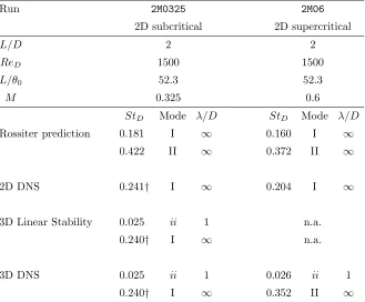
A Simulation Parameters 101 B Linear Stability Experiments 106 B.1 Influence of the Mach number . . . 107
B.2 Influence of the Reynolds number . . . 108
C Extension of the Linear Stability to Supercritical Conditions 111 C.1 Two-dimensional simulation of Rockwell experiment . . . 111
C.2 Linear stability results . . . 115
D Preliminary Results on 3D Wake Mode 119 D.1 Two-dimensional wake mode . . . 119
D.2 Three-dimensional simulations . . . 122
D.2.1 Flow field without spanwise disturbances . . . 122
List of Figures
1.1 Schematic of open cavity oscillations in compressible flows . . . 2
2.1 Basic configuration of the computational domain . . . 13
2.2 Visualisation of the computational grid . . . 14
2.3 Comparison of linear stability result with ARPACK solution . . . . 19
3.1 Vorticity field for run 2M06 (shear-layer mode) . . . . 23
3.2 Velocity field for run 2M06 (shear-layer mode) . . . . 24
3.3 Acoustic field for run 2M06 (shear-layer mode) . . . . 25
3.4 Vorticity contours and streamlines of the 2D steady base flow for different cavity aspect ratios . . . 26
3.5 Neutral stability curve and oscillation frequencies for run series H1 27 3.6 Neutral stability curve and oscillation frequencies for run series 2M 28 3.7 Neutral stability curve and oscillation frequencies for run series TK2 29 3.8 Neutral stability curve and oscillation frequencies for run series TK4 30 3.9 Long-time linear response of the cavity to 3D perturbations of dif-ferent spanwise wavelengths for run 2M0325 . . . . 32
3.10 3D linear stability results for run series2M . . . . 34
3.11 3D linear stability results for run seriesTK2M . . . . 35
3.12 3D linear stability results for run seriesH1 . . . . 36
3.13 Vorticity contours for 2D steady and time-averaged base flows . . . 38
x
3.15 3D visualisation of the flow for the unstable mode of spanwise
wave-length λ/D = 1 for the 3D linear run2M0325 . . . . 42
4.1 Streamlines and Rayleigh discriminant of 2D steady and time-averaged base flows . . . 45
4.2 Properties of the 2D steady base flow in runH1Re140for comparison with Couette flow . . . 51
5.1 Time trace of normal velocity for runs 2M0325 and 2M0325-3D. . . 57
5.2 Spectrum of the normal velocity for runs 2M0325 and2M0325-3D . 57 5.3 Spanwise velocities for run2M0325-3D . . . . 59
5.4 Time-averaged velocity field for runs 2M0325 and 2M0325-3D. . . . 60
5.5 Spanwise velocities for run2M06-3D . . . . 61
5.6 Time trace of streamwise velocity for runs 2M06 and2M06-3D . . . 63
5.7 Time trace of pressure for runs 2M06 and 2M06-3D . . . . 63
5.8 Time trace of spanwise velocity for run 2M06-3D . . . . 64
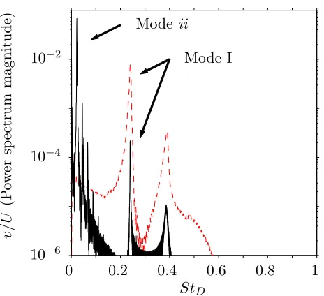
5.9 Power spectra of the streamwise velocity and pressure for runs2M06 and 2M06-3D . . . . 65
5.10 Power spectra of the spanwise velocity for run2M06-3D . . . . 66
5.11 Shear-layer spreading rates . . . 67
5.12 Reynolds stresses √u0u0/U, √v0v0/U, and √w0w0/U for runs 2M06 and 2M06-3D . . . . 69
5.13 Reynolds stressu0v0/U2 for runs 2M06and 2M06-3D . . . . 70
5.14 2D time-averaged velocity field for runs 2M06 and2M06-3D . . . . . 71
5.15 Sound pressure levels for runs2M06 and 2M06-3D . . . . 72
5.16 Vorticity fields for run2M0325-3D . . . . 74
5.17 Vorticity fields for run2M06-3D . . . . 75
5.18 Time trace of streamwise velocity for runsH1Re300and H1Re300-3D 77 5.19 Power spectra of the streamwise velocity for runs H1Re300 and H1Re300-3D . . . . 77
5.21 Power spectra of the spanwise velocity for runH1Re300-3D . . . . 79
5.22 Spanwise velocities for runH1Re300-3D . . . . 81
5.23 Time-averaged velocity and vorticity field for runH1Re300-3D . . . 82
6.1 Experimental visualisation of the spanwise structures by Rockwell & Knisely (1980) . . . 85
6.2 Visualisation of the slot cavitation by Ward (1973) . . . 87
6.3 Flow types in the slot cavitation experiment by Ward (1973) . . . 88
6.4 Experimental visualisation of the primary vortex by Faure et al. (2007) . . . 92
6.5 Experimental visualisation of the spanwise structures by Faureet al. (2007) . . . 93
6.6 Visualisation of the spanwise structures for runH1Re300-3D . . . . 94
C.1 Vorticity fields for runRkw . . . 113
C.2 Time trace at (x, y) = (0.5L,0) for runRkw . . . 114
C.3 2D time-averaged velocity field for runRkw . . . 115
C.4 Streamlines and Rayleigh discriminant of the 2D time-averaged base flow for run Rkw. . . 116
C.5 Schematics of the flow by Rockwell & Knisely (1980) . . . 117
D.1 Time trace of the pressure and velocities for run4M06wake . . . . 120
D.2 Spectrum of the normal velocity for run4M06wake . . . 121
D.3 Time trace of the drag coefficient for wake and shear-layer mode . 122 D.4 Time-averaged velocity fields and streamlines for wake and shear-layer modes . . . 123
D.5 Evolution of the spanwise vorticity for run4M06wake-3D . . . 124
D.6 Evolution of the vorticity for run4M06-3D . . . 126
D.7 Time trace of the pressure and velocities for run4M06-3D . . . 127
D.8 Time trace of the spanwise velocity for run4M06-3D . . . 127
xii
List of Tables
4.1 Critical conditions of the 3D centrifugal instability for flows over a backward-facing step, lid-driven cavity, Couette, and open cavity
flows . . . 53
5.1 Comparison of the dominant mode prediction for 2D and 3D runs with L/D= 2 . . . 56
5.2 Comparison of the dominant mode prediction for 2D and 3D runs with L/D= 1 . . . 78
A.1 Parameters and stability for the run seriesH1 . . . 102
A.2 Parameters and stability for the run series2M . . . 103
A.3 Parameters and stability for the run seriesTK2 . . . 104
A.4 Parameters and stability for the run seriesTK4 . . . 105
A.5 Parameters and stability for the run series4M . . . 105
B.1 Parametric study of the Mach number influence on the 3D linear stability . . . 108
Nomenclature
Roman characters
a Speed of soundcp Specific heat at constant pressure D Cavity depth
e Energy
k Thermal conductivity L Cavity length
M Mach number
Nx Number of computational grid points in the streamwise direction Ny Number of computational grid points in the normal direction Nz Number of computational grid points in the spanwise direction P Pressure
P r Prandtl number
q Vector of the conservative variables Re Reynolds number
ReD Reynolds number based onD ReL Reynolds number based onL Reθ Reynolds number based onθ StD Strouhal number based onD StL Strouhal number based onL T Temperature
xiv
U Freestream velocity u Streamwise velocity u Velocity vector v Normal velocity w Spanwise velocity x Streamwise direction y Normal direction z Spanwise direction
Greek characters
α Phase delay in Rossiter formula β Spanwise wavenumber
γ Ratio of specific heats
δω Shear-layer vorticity thickness η Rayleigh discriminant
θ Shear-layer momentum thickness
κ Average convection speed of vortical disturbances in Rossiter formula Λ Spanwise extent of the cavity
λ Spanwise wavelength of the 3D instability µ Dynamic viscosity
ν Kinematic viscosity ρ Density
σ Growth/damping rate of the 3D instability χ Merit function
Ω Complex eigenvalue of the 3D instability
ω Oscillation frequency of the 3D instability ωz Spanwise vorticity
Superscripts
¯ Time-averaged quantity
0
Perturbation quantity
d Dimensional quantity
Subscripts
∞ At infinity1
Chapter 1
Introduction
1.1
Motivation and review of previous work
From the canonical rectangular cut-out to more complicated shapes with internal structures, resonant cavity instabilities are endemic to a number of aircraft
com-ponents including weapon bays, landing gear wells, and instrumentation cavities. Self-sustained oscillations and intense acoustic loading inside the cavity can lead
to structural damage, optical distortion, and store separation problems. In partic-ular, weapons bay noise suppression has been a major motivation for recent work
on cavity flow, including active flow control to replace traditional passive devices such as spoilers, ramps, rakes, etc.
1.1.1 Rossiter mode
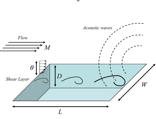
Dating back to the early work of Rossiter (1964), cavity oscillations in compressible
flow are typically described as a flow-acoustic resonance mechanism, as shown in figure 1.1: small instabilities in the shear layer interact with the downstream
corner of the cavity and generate acoustic waves, which propagate upstream and create new disturbances in the shear layer. For incompressible flow, the upstream
influence is instantaneous, while there is an acoustic delay for compressible flow. Resonance occurs at a given frequency when the disturbances lead to reinforcement
D
W
L
Acoustic waves
Shear Layer Flow
[image:17.612.171.439.76.281.2]M
Figure 1.1: Schematic of open cavity oscillations in compressible flows
Rossiter) mode, and can be distinguished from pure acoustic resonance where frequency selection depends only on the sound speed and geometrical parameters.
Rossiter (1964) performed an extensive set of experiments for two-dimensional rectangular cavities of different length to depth ratio, at different Mach numbers,
which identified a series of discrete frequencies of oscillation. He used the idea of the feedback process to develop a semi-empirical formula to predict the resonant
frequencies:
Stn= fnL U =
n−α
M+ 1κ n= 1,2,3... (1.1) where Stn is the Strouhal number corresponding to the n-th mode frequency,fn. The empirical constantsκandαcorrespond to the average convection speed of the vortical disturbances in the shear layer, and a phase delay (typically 1/κ= 1.75 and α= 0.25), respectively.
Data from a large number of experiments and simulations over the years show reasonable agreement with equation 1.1, but with significant scatter. The
3
can have a significant influence on the resonant frequencies and do not appear in Rossiter’s formula. Additionally, equation 1.1 does not give any indication of
whether such self-sustained oscillations do occur and, if so, which of several possible modes are present and if a particular mode (if any) is dominant.
1.1.2 Wake mode
Apart from the instability mechanism proposed by Rossiter, other modes of
oscilla-tion have been observed in cavity flows. In their incompressible experiment for an axisymmetric cavity, Gharib & Roshko (1987) observed a significant change in the
behavior of the cavity oscillation when the ratio of the cavity length relative to the upstream boundary layer momentum thickness was increased. Direct numerical
simulations by Rowleyet al. (2002b) showed similar results for a two-dimensional rectangular cavity. In this mode, the flow is characterized by a large-scale vortex
shedding from the cavity leading edge, similar to that observed behind bluff bod-ies, hence the term “wake mode” used to describe the resulting flow regime. As
the large vortex (dimension of the cavity depth) forms near the leading edge, free stream fluid enters the cavity and impinges on the cavity bottom. The vortex is
then shed from the leading edge and is violently ejected from the cavity, the all process resulting in a drastic increase in drag.
The wake mode transition has been observed in several two-dimensional numer-ical simulations (e.g., Fuglsang & Cain, 1992; Cainet al., 2000; Rowleyet al., 2002b;
Larsson et al., 2004), but experimental evidence of this mode is fairly limited. Three-dimensionality has been shown to play a role in suppressing the wake mode.
Large eddy simulations by Shieh & Morris (2000) showed that two-dimensional cav-ities in wake mode return to shear-layer mode when three-dimensional disturbances
are present in the incoming boundary layer. Similarly, recent work by Suponitsky
et al.(2005) showed that the development of a three-dimensional flow field,
gener-ated by the introduction of the random inflow disturbance into a two-dimensional cavity oscillating in wake mode, yielded the transition to the shear-layer mode,
highlight how a better understanding of the fundamental three-dimensional fea-tures of cavity flows is crucial to accurately connect numerical results, experiments
and practical applications.
1.1.3 Self-sustained versus forced oscillations
There are additional acoustic resonances of typical cavity geometries that lead, especially at lower Mach numbers and in confined laboratory experiments (e.g.,
wind tunnel resonance) to additional complications in the identification of cavity resonance mechanisms. Purely acoustic resonance can lead to a “detuning” and/or
reinforcement of the flow/acoustic shear layer modes. Rowleyet al.(2006) showed that oscillations observed in experiments are not always of the self-sustaining type
envisioned by Rossiter . Indeed, in many cases it appears that the cavity oscilla-tions are actually forced by boundary layer turbulence or other external sources
of noise. This clarification has major implications for the design of feedback con-trollers (e.g., Rowleyet al., 2002a). Recent models by Alvarez et al. (2004; 2005)
showed that there can be strong interactions with wind tunnel resonances, and confirm analytically that oscillations are not always self-sustaining.
1.1.4 Flow control
Over the past decades, two-dimensional cavity flows have received significant atten-tion (see for instance review articles from Rockwell & Naudascher, 1978; Colonius,
2001; Rowley & Williams, 2006), including several experimental and numerical studies at the California Institute of Technology (e.g., Krishnamurty, 1956; Saro-hia, 1975; Gharib, 1983; Rowley, 2001). Aside from numerical benchmarking, the
main motivations for studying cavity flow are noise reduction and flow control. Fundamental research has been conducted recently to examine how active
(open-and closed-loop) flow control can be use to replace traditional passive devices such as spoilers, ramps and rakes (e.g., Cattafesta III et al., 1999; Alvarezet al., 2004;
5
devices may be more effective for broadband noise reductions.
In analyzing the behavior of the shear layer oscillations, most investigators
have implicitly assumed that the shear layer behavior can be described in isola-tion, i.e., as if it were a free shear layer. In recent refinements to this model, Alvarez et al. (2004; 2005) have developed linear theory that couples the shear
layer dynamics and acoustic behavior of the cavity (essentially using an unsteady Kutta condition at the cavity leading and trailing edges), but non-parallel shear
layer effects and, in particular, the coupling of the flow inside the cavity have not been studied.
An alternative analysis of the global instability modes is to consider the basic, steady flow as two- or even three-dimensional. This viewpoint requires high-fidelity
steady flow solutions of the Navier-Stokes equations as input, and then solves a partial-derivative eigenvalue problem for 2D and 3D instabilities of the basic flow.
The underlying theory and methodology for extracting these bi- and tri-global instabilities are described by Theofilis (2003) in a recent review paper. Early efforts
have concentrated on incompressible flows, including backward-facing step, lid-driven cavities, laminar separation bubbles, etc. A significant accomplishment of
the present work has been to extend this effort to compressible flows where in many cases (including the cavity) small amplitude acoustic radiation is an important
aspect of the instabilities and must be treated with high-order-accurate numerics in order to avoid spurious oscillations or numerical dissipation of the relevant
instabilities.
1.1.5 Three-dimensionality in cavity flow
Recently, some aspects of the three-dimensional cavity flow have been
investi-gated using Large Eddy Simulation (LES) methods (Rizzetta & Visbal, 2003; Larchevˆeque et al., 2004; Chang et al., 2006) and Proper Orthogonal
Decomposi-tion (POD) (Podvin et al., 2006). These studies have been mainly focused on the frequencies of oscillation and coherence of the (two-dimensional) Rossiter modes,
mean flow and spectra. Some observations regarding the three-dimensionality of the large-scale turbulent structures are also reported but do not figure
promi-nently in these studies. Such LES data could be useful in future to examine the instabilities identified in this study at higher values of Reynolds number.
Likewise, three-dimensional experimental data is fairly limited but several
re-searchers have reported observations of three-dimensionality in cavity flows. Ahuja & Mendoza (1995) conducted an extensive set of experiments on the effect of
cav-ity dimensions, boundary layer, and temperature on cavcav-ity noise for subsonic flows with turbulent boundary layer upstream of the cavity. They determined that the
parameter L/W, the cavity length to width ratio, provided a transition between two- and three-dimensional flow. For L/W < 1, the cavity is classified as two-dimensional, as the flow was found to be uniform over much of the span, with a coherent shear layer spanning most of the cavity width. The cavity is said to be
three-dimensional forL/W >1, as the flow cannot maintain a coherent shear layer across its width because of the end-effects that cause significant spillage of flow over
the cavity side into the cavity. In that case, they reported three-dimensionality in the mean flow, and much lower (about 15 dB) acoustic loads than the
pre-dominately two-dimensional flow. However, Ahuja and Mendoza’s classification of wide cavities as two-dimensional is based on a time-averaged view of the flow field,
and the three-dimensionality is not related to the 3D instability we identify in our present work.
Three-dimensional flow features have also been observed for wide cavities in early wind tunnel experiments at low subsonic velocities by Maull & East (1963).
Using oil flow visualisation of surface streamlines at the bottom of the cavity and surface static-pressure distributions, they showed the existence, under certain
conditions, of nearly steady spanwise cellular pattern within the cavity. They observed that the width of each cell remained essentially independent of the total
cavity span but that the most regular pattern existed when the cavity span was an integral number of preferred cell-width. Rockwell & Knisely (1980) also observed
7
cavity with laminar boundary layer upstream. A hydrogen bubble technique was used to visualise the spanwise structure in the cavity. More evidence of
three-dimensional structures in cavity flows have been presented in the recent work of Faure et al. (2007). The physics of these features has yet to be fully understood.
In conclusion, while observations of three-dimensionality in cavity flow have been reported, the physics of these features has yet to be fully understood. As
a result, past efforts on cavity flow control have typically ignored non-parallel and three-dimensional effects. These approaches may, on one hand, reduce the
effectiveness of model-based control, or on the other hand disregard important three-dimensional mechanisms that could be exploited in passive ways to reduce
broadband noise.
1.2
Overview of present work
The focus of the present work is therefore to characterize the basic instabilities of three-dimensional open cavity flows. Because the basic (steady or time-averaged)
cavity flow is complex and non-parallel, our stability analysis is focused on ex-tracting global instabilities from Direct Numerical Simulations (DNS) of the full
and linearized compressible Navier–Stokes equations.
From the start, it must be acknowledged that accurate computation of realistic,
unsteady, three-dimensional aircraft cavities, at realistic flight Reynolds numbers, is well beyond current computer resources. While realizable parameter regimes (es-pecially small scale experiments) may be reached with LES, such computations are
sufficiently time consuming that they prohibit a significant portion of parameter space from being investigated. By focusing our attention on low Reynolds number
direct numerical simulations of 2D and 3D spanwise periodic flows, we are able to examine a large parameter space (Mach number, cavity dimensions, boundary
shear layer oscillations in cavity flows using inviscid parallel flow stability. Models and computations at low Reynolds numbers display the same instabilities as the
inviscid analysis.
As we show that the principle effect of the Reynolds number is to damp the instabilities, any instabilities observed here are likely to be at play at full-scale
Reynolds numbers. Thus the low Reynolds number analysis and simulations can bracket the behaviors that exist in experiments and flight conditions, and at the
same time understand in detail the instabilities and their parametric variations. In general, simulations of simpler (even two-dimensional) flows can lead to insights
into the flow physics that directly carry over to full-scale complex flows, and provide data for control and modeling efforts.
In the present work, we consider two- and three-dimensional instabilities to basic cavity flows that are homogeneous in the spanwise direction, for low to
mod-erate Reynolds numbers. Chapter 2 gives an overview of the numerical methods and the linear stability theory used in this study.
First, the onset of two-dimensional cavity instability is characterized as a func-tion of Reynolds number, Mach number, cavity aspect ratio, and incident
shear-layer thickness. The two-dimensional modes are consistent, both in terms of oscilla-tion frequency and eigenfuncoscilla-tion structure with the typical Rossiter flow/acoustic
resonant modes that have been observed in many cavity experiments and flight tests. For basic cavity flows that are two-dimensionally stable, we then search
for three-dimensional instabilities of the steady base flow, and identify, for the first time, the presence of such instabilities. The 2D and 3D modes, and their
properties, are discussed in chapter 3.
For cavity length-to-depth ratios of 1, 2, and 4 considered here, the instability
appears to arise from a generic centrifugal instability mechanism associated with the internal recirculation vortical flow that occupies the downstream part of the
cavity. The three-dimensional instabilities are related to centrifugal instabilities reported in flows over backward-facing steps, lid-driven cavity flows, and Couette
9
A few selected three-dimensional numerical simulations of the full compressible Navier–Stokes equations are then performed. To our knowledge, this is the first
time that strict DNS of three-dimensional compressible cavity flows have been reported. The results, in chapter 5, exhibit three-dimensional features in good agreement with the linear analysis predictions, both in terms of spanwise structures
and oscillation frequencies.
In chapter 6, we discuss the connections between the 3D instabilities we report
here and observations of three-dimensionality in previous numerical studies and experiments. Our numerical results are consistent with low-frequency modulations
and spanwise structures reported in previous studies on open cavity flows. In particular, visual evidence of the 3D mode is found in recent low Reynolds number
Chapter 2
Numerical Methods and Stability Theory
2.1
Direct numerical simulations
Following previous work of Rowley et al. (2002b) on cavity flows, we develop a DNS code to solve the full compressible Navier–Stokes (NS) equations and study
the flow over three-dimensional open cavities. The equations are solved directly, meaning that no turbulence model is used and all the scales of the flow are
re-solved. The Navier–Stokes equations are written in conservative form as follows:
∂ρ ∂t +
∂
∂xj(ρuj) = 0 ∂ρui
∂t + ∂
∂xj(ρuiuj+P δij) = 1 Re ∂ ∂xj( ∂ui ∂xj + ∂uj ∂xi − 2 3 ∂uk ∂xkδij) ∂e
∂t + ∂ ∂xj
((e+P)uj) = 1 Re ∂ ∂xj (ui(∂ui ∂xj +∂uj ∂xi −
2 3
∂uk ∂xk
δij)) + 1 Re
1 P r
∂2
T ∂xk∂xk
(2.1)
with the equation of state
P = γ−1 γ ρT,
where ρ, P, and T are the density, pressure, and temperature, and ui is the velocity in the direction of the Cartesian coordinate xi. The energy e is defined by e = ρ(E+|u|2
11
freestream property.
ρ= ρ d
ρ∞
P = P d
ρ∞a2∞
T = T
dcp
a2
∞
e= e d
ρ∞a2∞
ui = u d i a∞
xi= x d i
D t=
tda
∞
D
Here,γ is the ratio of specific heats,cp the specific heat at constant pressure,athe speed of sound, and D the cavity depth. The Prandtl number and the Reynolds numbers are defined respectively as
P r= cpµ∞
k Re=
ρ∞a∞D
µ∞
Reθ = ρ∞U∞θ0 µ∞
,
where k is the thermal conductivity, µ the dynamic viscosity and θ0 the initial
boundary layer momentum thickness at the cavity leading edge.
A linearized version of the equations is also implemented: we assume that the
flow field q = [ρu, ρv, ρw, ρ, e]T can be decomposed into q = q¯+q0
, where ¯q is a steady solution of the equations and the perturbation field q0
verifies q0
¯q. The Navier–Stokes equations are then linearised about q¯ by neglecting higher-order terms in q0
to give a first-order approximation. The perturbation field now
satisfies
∂ρ0
∂t + ∂ ∂xj(¯ρu
0
j+ρ
0
¯ uj) = 0 ∂
∂t(¯ρu
0
i+ρ
0
¯ ui) + ∂
∂xj
(¯ρ( ¯uiu0
j+u
0
iuj) +¯ ρ
0
¯
uiuj¯ +P0
δij) = 1 Re ∂ ∂xj (∂u 0 i ∂xj +∂u 0 j ∂xi −
2 3 ∂u0 k ∂xk δij) ∂e0 ∂t + ∂
∂xj((¯e+ ¯P)u
0
j+ (e
0
+P0
) ¯uj) = 1 Re
∂ ∂xj( ¯ui(
∂u0 i ∂xj + ∂u0 j ∂xi − 2 3 ∂u0 k ∂xk δij) +u0
i(
∂u¯i ∂xj +
∂u¯j ∂xi −
2 3
∂u¯k ∂xkδij)) + 1 Re 1 P r ∂2 T0
∂xk∂xk
The existing DNS code can solve linear or nonlinear NS equations for both two-dimensional and three-two-dimensional flows. The equations are solved on a structured
mesh, using a sixth-order compact finite-difference scheme for spatial discretization in the x- and y-direction (Lele, 1992), and a fourth-order Runge-Kutta algorithm for time-marching. The cavity is supposed homogeneous (periodic) in the
span-wise direction (z-direction) and the derivatives are computed using Fast Fourier Transform (FFT) method with subroutines provided by the FFTW library (Frigo
& Johnson, 1997-2007). The boundary conditions are non-reflective for the inflow and outflow, no slip, and constant temperature (T =T∞) at the walls (Thompson,
1990; Poinsot & Lele, 1992). In addition, a buffer zone is implemented at the in-flow, outin-flow, and normal computational boundaries to reduce acoustic reflections
(Coloniuset al., 1993; Freund, 1997). Unless stated otherwise, the simulations are initiated with a Blasius flat-plate boundary layer spanning the cavity and zero flow
within the cavity.
The code can handle any type of block geometry and is fully parallelized
us-ing Message-Passus-ing Interface (MPI). The simulations were performed on high-performance Beowulf clusters at the California Institute of Technology. Additional
computer resources were provided by the Air Force Office of Scientific Research (AFOSR) and the Army Research Laboratory (ARL).
The cavity configuration and flow conditions are controlled by the following parameters: the cavity aspect ratio L/D and spanwise extent Λ/D, the ratio of the cavity length to the initial boundary layer momentum thickness at the leading edge of the cavity L/θ0, the Reynolds number Reθ =U θ0/ν, and the freestream
Mach numberM =U/a∞(see figure 2.1). As temperature differences are expected
to remain small, the transport properties are assumed constant: we set P r = 0.7 and γ = 1.4, the values for air.
Typical grid sizes ranged from a few hundred thousand to several million grid
points. Each spanwise wavenumber is discretized on a stretched Cartesian grid, with clustering of points near the walls and the shear layer spanning the cavity.
13
z y
x L
D U
Inflow
Outflow
Outflow Buffer zone
PSfrag replacements Λ
x
y
z
Figure 2.1: Basic configuration of the computational domain
win 3D) at every time step. For 2D simulations, three approximately equi-spaced probes are located in the shear layer aty= 0, and three more at the same stream-wise positions inside the cavity at y =−0.5D. Additional probes in the spanwise cross-section z = 0.5Λ and equally spaced along the span in the shear layer at (x, y) = (0.5L,0) are considered for 3D simulations. Figure 2.2 shows a typical 3D
grid and the location of the probes.
On a side note, we also report that the numerical code we developed has been successfully used to investigate other problems than cavity flows. Gudmundsson
& Colonius (2006) adapted the code to study jet noise and the linear stability characteristics of the mean velocity profiles produced by chevron nozzles. Burnes & Colonius (2007) are implementing a Large Eddy Simulation version of the code
to investigate the mixing and flame-holding characteristics of cavity flows at high Reynolds numbers. Future applications of the code also include simulations of
-2
0
2
4
6
2 1 0 0 2 4
y
z
x
15
2.2
Linear stability theory
Based on the assumption that the shear layer may be decoupled from the acoustic
scattering and recirculating flow in the cavity, the classical approach to study the stability of cavity flow uses the theory of linear stability of parallel shear flow.
The equations of motions are linearized about a parallel mean flow (known basic flow, only function of one spatial direction) and the fluctuations are written in
normal mode form. In general, this formulation leads to an eigenvalue problem and a dispersive relation, which relates frequencies of the perturbations to their
corresponding wavenumber. For the classical approach, non-parallel effects are only included through the introduction of a quasi-parallel (or Parabolized) stability
approach that cannot account for the effects of the leading and trailing cavity edges (and their acoustic coupling to the hydrodynamic disturbances). Recent work
by Alvarez et al. (2004; 2005) has extended the parallel flow stability analysis to include the scattering/receptivity/acoustic feedback by using a Weiner-Hopf
technique, but non-parallel and three-dimensional effects have not been considered. An alternative analysis, called bi-global linear stability theory, has been used
for non-parallel flows (Theofilis & Colonius, 2003; Theofilis et al., 2004; Theofilis, 2003). In this approach, the transient solution of the equations of motion q = [ρu, ρv, ρw, ρ, e]T is decomposed into
q(x, y, z, t) =q¯(x, y) +q0
(x, y, z, t), (2.3)
where q¯(x, y) is the unknown steady two-dimensional basic flow and q0
(x, y, z, t) an unsteady three-dimensional perturbation with ||q0
|| ||¯q|| . As the domain is homogeneous in the spanwise direction, a general perturbation can be decomposed into Fourier modes with spanwise wavenumbers β. At linear order, modes with different wavenumbers are decoupled and the following eigenmode Ansatz can be introduced:
q0
(x, y, z, t) =X n
ˆ
where the parameterβ is taken to be a real and prescribed spanwise wavenumber, related to a spanwise wavelength in the cavity byλ= 2π/β,qˆnand Ωn=ωn+iσn are the unknown complex eigenmodes and corresponding complex eigenvalues, both dependent on β. Complex conjugation is required in equation (2.4) since q0
is real. The frequency and the growth/damping rate of the mode are given
by ωn and σn, respectively. The long-time behavior of the linear solution will be dictated by the mode with the eigenvalue Ω = ω+iσ of largest imaginary part. The flow is said to be subcritical (stable) if σ is strictly negative, neutrally stable ifσ = 0, and supercritical (unstable) ifσ >0.
Eventually, the determination of the least damped (or most unstable) modes for a given wavelength β amounts to finding the eigenvalue Ω and corresponding eigenvector by integrating the governing equations directly in the time domain.
2.3
Residual method and L2 fitting routines
To determine the least-damped eigenvalue practically, a least-squares fitting method (Press et al., 1992) is applied to the data time history when exponential decay or
growth was reached: given the long-time evolution of the vector field q0
at any location (x0, y0, z0) and an initial guess for the unknown parameters¯q(x0, y0, z0),
ˆ
qr(x0, y0, z0), qˆi(x0, y0, z0), ω, and σ, a set of “best-fit” parameters is computed
such that the “merit function”χ, which measures the agreement between the data and the model (with a particular choice of parameters), is minimized. In our case, the model depends nonlinearly on a set (ak, k = 1,2, ..., M) of unknown parame-ters and the “merit function” χ is defined as
χ2 =
Nf it
X
i=1
datai−X(a1, a2, ..., aM, ti)
σi
2
,
17
Following equation (2.4), the “merit function” takes the form
χ2= N X
i=1
q0
(x0, y0, z0, ti)−(a1+ (a4cosa2ti−a5sina2ti)ea3ti
2
.
Note that the method is sensitive to the initial guess (same order of magnitude as the “best-fit” parameters needed for accurate results) and the length of data
to fit (namely, if N is too large and the data still contains transient components, the fit may not be successful). Upon convergence, the mode frequencyω =a2 and
growth/damping rate σ = a3, which are independent of the location (x0, y0, z0),
can be recovered.
With the eigenvalue determined, equation (2.4) may be written at three differ-ent times,t1,t2=t1+ ∆t, andt3=t1+ 2∆tas a linear system of three unknowns
¯
q, ˆqr, and qˆi. With the transient solution qn = q(x, y, z, tn) available at these
times, the system can be solved to deliver the steady-state solution ¯q and the spatial structure (qˆr,ˆqi) of the linear eigenmode:
¯
q = q1e
2σ∆t−2q
2eσ∆tcosω∆t+q3
e2σ∆t−2eσ∆tcosω∆t+ 1 (2.5) ˆ
qr =
s1(q2−¯q)−s2(q1−q¯)
c2s1−c1s2
(2.6)
ˆ qi =
c1(q2−q¯)−c2(q1−¯q)
c2s1−c1s2
(2.7)
where
c1 =eσt1cosωt1 c2 =eσt2cosωt2 s1=eσt1sinωt1 s2 =eσt2sinωt2.
2.4
ARPACK
To validate the linear stability results, a direct approach was also considered,
through long-time integration. Following the nomenclature introduced in §2.2, for a given wavenumber β, the three-dimensional linearized NS equations can be written symbolically in matrix notation as
∂q0
∂t =A
∂ ∂x,
∂ ∂y,¯q
q0
, (2.8)
where q0
is the vector of the perturbed conservative variables and A is a spatial differential operator depending on the base flow and cavity parameters (aspect
ra-tio, spanwise wavenumber, Re, etc.). Once the equations are spatially discretized, we may represent this equation as:
∂q0
∂t =Aq
0
, (2.9)
where now q0
is the discretized solution vector (length 5N whereN is the number of grid points), and A is a constant real 5N by 5N matrix. In this discrete ap-proach, the matrixAis a function of the (discretized) known steady flow¯qand the simulation parameters. The stability of this ordinary differential equation depends on the eigensystem ofA. The eigenvalues (λn, n= 1, N) areNnot necessarily dis-tinct solutions of det(A−λI) = 0, and the corresponding eigenvectors xn are the linearly independent solutions of Axn=λnxn. For the non-defective cases where there are N linearly independent eigenvectors, X−1
= [x1, x2, ..., xN]−1 exists and
the solution can be written symbolically as
q0
=eAtq0
0, (2.10)
where q0
0 is the initial perturbation and
eAt=Xdiag[eλ1t , eλ2t
, ..., eλNt]X−1
. (2.11)
19
PSfrag replacements 0
0 1
1
2
-x y
PSfrag replacements 0
0 1
1
2
-x
y
(a) (b)
Figure 2.3: Contours of the streamwise velocityu0
/U for the dominant eigenmode of spanwise wavelength λ/D = 1 for run 2M0325: ( ) ARPACK solution;
( ) Linear stability result; (a) real part; (b) imaginary part
conclusion stands if the system is defective. Comparison of equations (2.4) and
(2.11) reveals that the continuous and discrete formalisms are simply related by λm =−iΩ. Given a cavity configuration and flow conditions, the eigenvalue of A with largest real part (i.e., the least damped or fastest growing three-dimensional mode) could theoretically be directly computed using ARPACK, as well as the corresponding eigenvector, to visualise the shape of the instability.
In practice, the use of ARPACK was significantly limited by the size and com-plexity of our problem. The software was therefore only used here to validate our
time-domain methods. As expected, the dominant eigenmode and corresponding eigenvalue computed with ARPACK for the same test case were in excellent
agree-ment with the results of the linear stability analysis, as shown in figure 2.3. Both methods predicted three-dimensional instabilities with less than 1% difference on
the mode growth rate and frequency.
2.5
Validation
simple acoustic problems and previous validated numerical results from Rowley
et al.(2002b). The two-dimensional basic flow calculations are performed on fine
grids (about half a million to a million grid points) and for supercritical cases, the oscillation frequencies are in good agreement with Rossiter mode frequencies, as further discussed in §3.1.2).
Additionally, the 2D simulation 2M06-K reproduces one of the experimental
configurations of Krishnamurty (1956) with laminar incoming boundary layer. The
flow parameters (L/D = 2, M = 0.6, L/θ0 = 80, ReD = 1500) match the
condi-tions of the experiment (apart from the Reynolds, which is higher by about a factor
20 in the experiment). We find good qualitative agreement between the structure of the radiated acoustic field and schlieren pictures from the experiment. The
measured frequency is f ≈ 29 000 Hz, which corresponds to a Strouhal number StL=f L/U ≈0.73. This result matches the oscillation frequency StL= 0.723 in our numerical simulation (see appendix A). Using optical interferometry, Krish-namurty (1956) estimated the sound pressure levels (SPL) to approximately 163
dB for different cavity configurations. This value is similar to the SPL we measure and report in chapter 5.
For the stability analysis, it is particularly important to verify that the modes observed are physical and not generated by any numerical artifact. Several initial
conditions with disturbances at different locations in the cavity were considered in order to perturb the linear equations and study the flow response. Similarly,
to demonstrate grid convergence of the three-dimensional stability computations, simulations were performed on a finer grid for the same test case. As expected for
a global instability, the dominant three-dimensional mode is independent of the initial perturbation and grid spacing, as both the nondimensionalised frequency
21
Chapter 3
Linear Stability Results
As described in chapter 2, the three-dimensional linear stability analysis relies on
the existence of subcritical conditions with a steady two-dimensional basic flow ¯
q(x, y), an exact solution of the 2D NS equations. However, for most experiments and realistic flight conditions, the flow parameters would be such that Rossiter modes do occur and eventually saturate into a periodically oscillating flow. It must be acknowledged that the presence of three-dimensional instabilities is likely
to alter the two-dimensional basic flow on which the present linear analysis is based. With this in mind, our approach here is to investigate the three-dimensional linear
stability of a given base flow, regardless of potential interactions. Such approach has been widely used to predict the stability and growth rate of boundary layers,
for instance. As discussed in chapter 5 and chapter 6, the features observed in the linear results are in fact relevant to full nonlinear simulations and experiments.
Potential extension of the linear stability analysis to supercritical conditions is presented in appendix C.
3.1
Two-dimensional simulations
The first step of the linear stability analysis is to characterize the onset of
3.1.1 Shear-layer mode
As discussed in the introduction, the shear-layer (Rossiter) mode is characterized by a flow-acoustic feedback process. Small disturbances in the shear layer are
amplified as they advect downstream through the shear layer and generate acoustic waves upon impingement on the downstream edge of the cavity. These acoustic
waves propagate back upstream and interact with the shear layer to excite further instabilities.
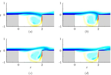
This mechanism is clearly observed in the 2D simulations. The vorticity, veloc-ity and acoustic fields for run2M06(L/D= 2,L/θ0 = 52.8,M = 0.6,ReD = 1500)
are shown in figures 3.1, 3.2, and 3.3 respectively. They are representative of all
the simulations with shear-layer mode oscillations. As mentioned in the validation section in §2.5, good qualitative agreement is obtained between the density
fluc-tuations observed in the simulations and schlieren pictures from experiments (e.g., Krishnamurty, 1956). In the present case, the roll-up of vorticity in the shear
layer can be observed, but there is no shedding of vortical disturbances before impingement at the downstream cavity edge. In general, the velocity magnitude
inside the cavity is only a fraction of the freestream velocity (less than 10% for subcritical conditions and up to 30% for supercritical conditions) and the internal
flow is relatively weak.
One important feature of the cavity flow is the recirculating vortical flow (also
commonly referred as primary vortex) in the downstream half of the cavity. This vortex is present in the steady state for subcritical conditions and in a
time-averaged sense for supercritical conditions. Figure 3.4 shows the 2D steady base flow for different cavity configurations. As further discussed in§3.2, the
23
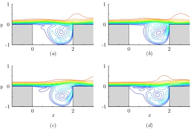
0 2
-1 0 1
y
0 2
-1 0 1
(a) (b)
0 2
-1 0 1
y
x 0 2
-1 0 1
x
[image:38.612.112.499.235.498.2](c) (d)
Figure 3.1: Vorticity field for the shear-layer mode (run 2M06) at four different
times (a-d) corresponding to approximately a quarter of a period of oscillation; 21
0 2 -1
0 1
y
0 2
-1 0 1
(a) (b)
0 2
-1 0 1
y
x 0 2
-1 0 1
x
[image:39.612.110.499.237.499.2](c) (d)
Figure 3.2: Velocity field for the shear-layer mode (run 2M06) at four different
times (a-d) (same times as in figure 3.1); 19 equi-spaced contours of the velocity
25
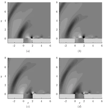
-2 0 2 4 6
0 2 4 6 8
y
-2 0 2 4 6
0 2 4 6 8
(a) (b)
-2 0 2 4 6
0 2 4 6 8
y
x -2 0 2 4 6
0 2 4 6 8
x
[image:40.612.108.504.162.572.2](c) (d)
Figure 3.3: Visualisation of the acoustic field for the shear-layer mode (run2M06)
PSfrag replacements 0 0 1 1 1 2 4 0.4 -x y PSfrag replacements 0 0 1 1 2 4 0.4-x y PSfrag replacements 0 0 1 1 2 4 0.4 -x y
(a) (b) (c)
Figure 3.4: Vorticity contours and streamlines of the two-dimensional steady base
flow; Ten equally-spaced contours betweenωzD/U =−1 and 1 are shown: (a) run
H1Re200; (b) run2M03; (b) runTK4M03Re65. In each case, the shear-layer and the
primary vortex within the cavity are clearly identified.
3.1.2 Neutral stability curves
While Rossiter’s formula in equation 1.1 provides reasonable predictions for the
frequency of oscillations that occur in self-sustained oscillations, it says nothing about whethersuch oscillations do occur and, if they do, which of many possible
unstable modes is selected, and at what amplitude such oscillations would saturate. For the most part, it can be presumed that at realistic flight-values the
parame-ters M,Reθ,L/D, and L/θ would be such that oscillations do indeed occur. The critical values of, for example, the Reynolds at which the flow first becomes
un-stable is quite low. Nevertheless, it turns out that understanding the behaviour of the instability near this critical transition has important consequences for cavity
oscillations at realistic Reynolds numbers.
The parameters for the different runs and the stability results are tabulated in
appendix A. Given a cavity configuration and different flow conditions, several two-dimensional simulations are performed to construct the estimated neutral stability
curve for the two-dimensional instabilities of the basic cavity flow (e.g., figures 3.5, 3.6, 3.7, and 3.8(a)). The DNS results are classified according to whether the flow
is two-dimensionally stable (and thus a steady-state solution can be obtained) or whether the flow results in self-sustaining oscillations. The oscillation frequencies
27 PSfrag replacements
3D unstable
2D & 3D stable
2D unstable 2000 4000 6000 8000 10000 6000 0.1
0.2 0.3 0.4 0.5 0.6
0.1 0.2 0.4 0.6 0.8 1 M ReD S t L
Rossiter mode I
Rossiter mode II
PSfrag replacements 3D unstable 2D & 3D stable
2D unstable 2000 4000 6000 8000 10000 6000 0.1 0.2
0.3 0.4 0.5 0.6 0.1 0.2 0.4 0.6 0.8 1 M R e D StL
Rossiter mode I
Rossiter mode II
(a) (b)
Figure 3.5: Results for cavity run seriesH1(L/D= 1,L/θ0 = 23.2): (a) Schematic
of the neutral stability curve from 2D nonlinear simulations (2D stable ( ) and unstable ()) and from the 3D linear analysis in§3.2 (3D stable (◦) and unstable
( • )); (b) Strouhal numbers StL = f L/U for the supercritical conditions in (a), compared to equation 1.1. Only one dominant mode ( N) is present in this case.
The results of the three-dimensional linear stability analysis from§3.2 are also presented in figures 3.5, 3.6, 3.7, and 3.8(a). The different shaded regions indicate
the approximate stability transitions. The critical conditions are estimated by linear interpolation between stable and unstable conditions. Here, it must be
acknowledged that these figures represent a general stability trend rather than precise computation of critical conditions. Also, the 3D stability is based on linear
results and is therefore not available for supercritical conditions (i.e., the region of 2D instability). However, the results of our nonlinear simulations, discussed in chapter 5, tend to indicate that the critical conditions for the onset of the 3D
instability are similar on both sides of the 2D stability transition.
The two-dimensional results are consistent with the typical flow/acoustic
res-onant modes that have been observed in many cavity experiments (e.g., Krishna-murty, 1956; Rossiter, 1964; Sarohia, 1975; Heller & Bliss, 1975; Tam & Block,
two-28
3D unstable
2D & 3D stable
2D unstable 1000 1250 1500 1750 2000 0.1
0.2 0.3 0.4 0.5 0.6 0.1 0.2 0.4 0.6 0.8 1 M ReD S t L
Rossiter mode I
Rossiter mode II
3D unstable 2D & 3D stable
2D unstable 1000 1250 1500 1750 2000 0.1 0.2
0.3 0.4 0.5 0.6 0.1 0.2 0.4 0.6 0.8 1 M R e D StL
Rossiter mode I
Rossiter mode II
(a) (b)
Figure 3.6: Results for cavity run series2M(L/D= 2,L/θ0 = 52.8): (a) Schematic
of the neutral stability curve from 2D nonlinear simulations (2D stable ( ) and unstable ()) and from the 3D linear analysis in§3.2 (3D stable (◦) and unstable
( • )); (b) Strouhal numbers StL = f L/U for the supercritical conditions in (a), compared to equation 1.1: ( N) dominant mode, ( ×) subdominant mode
dimensional instability is essentially of the Rossiter type, wherein Kelvin-Helmholtz instabilities in the shear layer spanning the cavity are coupled to acoustic
feed-back and receptivity at the trailing and leading edges, respectively. Frequencies of oscillation are found to be predicted by Rossiter’s formula to within the
exper-imental scatter of measurements that have been made over the years for cavities with laminar and turbulent boundary layers.
The onset of Rossiter mode as a function of the parameters is typically summa-rized qualitatively as follows: there is a critical value of M,Reθ, and L/θ beyond which oscillations occur. There does not appear to be any critical value of L/D in the range of parameters considered 1 < L/D < 6. The stability results from the two-dimensional simulations are consistent with these general trends. For low
Reynolds number and Mach number, the flow is subcritical and ultimately reaches a steady state. As these parameters, or the ratio of the cavity length to the
ini-tial boundary layer momentum thickness L/θ0, are increased, the flow becomes
29
PSfrag replacements
3D unstable
2D & 3D stable 2D unstable 1000 2000 3000 4000 5000 6000 0.1
0.2 0.3 0.4 0.5 0.6 0.1 0.2 0.4 0.6 0.8 1 M ReD S t L
Rossiter mode I
Rossiter mode II
PSfrag replacements 3D unstable 2D & 3D stable
2D unstable 1000 2000 3000 4000 5000 6000 0.1 0.2
0.3 0.4 0.5 0.6 0.1 0.2 0.4 0.6 0.8 1 M R e D StL
Rossiter mode I
Rossiter mode II
(a) (b)
Figure 3.7: Results for cavity run series TK2 (L/D = 2, L/θ0 = 30.12): (a)
Schematic of the neutral stability curve from 2D nonlinear simulations (2D
PSfrag replacements
3D unstable
2D & 3D stable
2D unstable 400 600 800 1000 1200 0.1
0.2 0.3 0.4 0.5 0.6
0.1 0.2 0.4 0.6 0.8 1 M ReD S t L
Rossiter mode I
Rossiter mode II
PSfrag replacements 3D unstable 2D & 3D stable
2D unstable 400 600 800 1000 1200 0.1 0.2
0.3 0.4 0.5 0.6 0.1 0.2 0.4 0.6 0.8 1 M R e D StL
Rossiter mode I
Rossiter mode II
(a) (b)
Figure 3.8: Results for cavity run series TK4 (L/D = 4, L/θ0 = 60.24): (a)
Schematic of the neutral stability curve from 2D nonlinear simulations (2D
31
As mentioned in the previous section, the parameters L/D, L/θ0, and Reθ
affect the oscillation frequencies, and in particular the selection of a particular
resonant frequency. For instance, in figure 3.6, the flow is stationary for run 2M03
atM = 0.3 andReD = 1500. The regime of shear-layer oscillations can be reached by either increasing the Reynolds number (i.e., run2M03Re80) or the Mach number
(i.e., run 2M04). Here, the resonant frequency corresponds to a Rossiter mode II
in the first case and mode I in the latter. In general, higher Rossiter modes are
observed for larger L/θ0 and higher Mach number (see appendix A).
3.2
Three-dimensional linear stability
The neutral stability curves presented in the previous section (3.1) are the starting point of the three-dimensionallinear stability analysis: the goal here is to
investi-gate whether or not 3D instability takes place before the onset of 2D instabilities. For subcritical cases, the two-dimensional steady flow ¯q is extracted from the DNS and used as base flow for the linear three-dimensional simulations: as initial condition, a perturbation of given wavelength λ(therefore looking at oneβ-mode at a time) is added to ¯q and the 3D linearised Navier–Stokes equations are solved. The least damped (or most unstable) eigenmode (e.g., figure 3.14) and the
corre-sponding eigenvalue Ω =ω+iσare then determined from the long-time response of the cavity (e.g., figure 3.9) . The nondimensionalised growth/damping rateσD/U and Strouhal numberStD =ωD/2πU are computed in each case for a set a discrete spanwise wavelength (e.g., figure 3.10) and the stability of the three-dimensional mode is reported back on the stability curve.
3.2.1 Three-dimensional mode properties
Figures 3.10, 3.11, and 3.12 show the growth/damping rate and frequency of the dominant three-dimensional mode as a function of the spanwise wavelength, for
500 400
300 200
100 0
10−6
10−4
10−2
10 0
log(|u|/U)
tU/D
lo
g
|
u
’
/
U
|
Figure 3.9: Long-time linear response of the cavity to three-dimensional
pertur-bations of different spanwise wavelengths for run 2M0325 at (x, y, z) = (L/2,0,0):
( ) λ/D = 0.5, ( ) λ/D = 1, ( ) λ/D = 1.5, ( 4 ) λ/D = 2. This figure is a typical output of the linear stability simulations. Here, the disturbance of spanwise wavelength λ/D = 1 is growing exponentially while the disturbances at other wavelengths are damped.
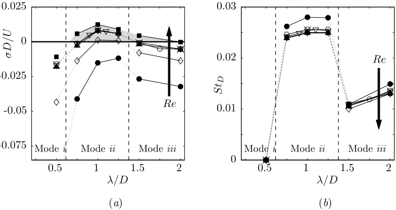
aspect ratio L/D= 1,L/D= 2, andL/D= 4 considered here (see appendix A) For a band of spanwise wavelengths around the size of the cavity depth (λ/D≈ 1), the dominant mode has a positive growth rate under certain conditions. This
unstable mode (referred as Mode ii) is unsteady and the oscillation frequency based on the cavity depth D are comparable in all cases. This suggests that D, rather thanLorθ0, is the most appropriate length scale to characterize the
three-dimensional instability. By contrast, the two-three-dimensional unstable Rossiter mode
has frequency f L/U scaling with the cavity length: in this feedback process, the resonant frequencies are directly connected to the times for vortical structures and
33
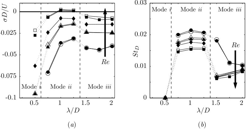
Aside from this oscillatory mode, the presence of other three-dimensional modes is suggested in figures 3.10, 3.11, and 3.12. In particular, the linear stability of the
shortest cavity L/D= 1 differs from the other cases. As the Reynolds number is increased, the first mode to become unstable is steady (StD = 0) and has a smaller spanwise wavelength (λ/D ≈0.5). A similar steady mode (referred as Modei) is
observed for cavities of larger aspect ratio but is not amplified. We argue that the specific properties of the three-dimensional mode for the square cavity are related
to the recirculating vortical flow that occupies the whole cavity in that particular configuration. These features are discussed in more detail in chapter 4.
Finally, the linear stability results also suggest the presence of another unsteady mode of larger spanwise wavelength λ/D ≥1.5. However, this mode iii does not have the largest linear growth rate at any of the conditions considered here, and is not observed in the three-dimensional nonlinear simulations we performed. For
several cases, a more extensive set of spanwise wavelength was also considered (0.1≤λ/D ≤32), but did not lead to any additional instabilities.
3.2.2 Parameter dependence
As mentioned previously, the parametersL/D,L/θ0,ReD, andM control the
on-set of the shear-layer (Rossiter) oscillation and whether the steady two-dimensional
flow needed for the linear analysis exists or not. Within the domain of 2D stabil-ity, our linear results show that the flow parameters affect the properties of the
three-dimensional modes in four aspects. First, as discussed above, the cavity as-pect ratio controls which mode (namely i or ii) is the dominant mode; secondly,
the Reynolds number has a direct effect on the growth rate as viscosity plays a stabilizing role; thirdly, a change in certain parameters (e.g., L/θ0 and Re)
mod-ifies the strength of the recirculating region in the two-dimensional base flow and
indirectly the mode growth rate and frequency; and finally, the Mach number has
PSfrag replacements
Modei Mode ii Mode iii
-0.05 -0.025 0 0.025 -0.075 0.01 0.02 0.03 2
0.5 1 1.5
λ/D σ D /U StD Re λ/D PSfrag replacements
Modei Modeii Modeiii
-0.05 -0.025 0 0.025 -0.075 0.01 0.02 0.03 2
0.5 1 1.5
λ/D σD/U S tD Re λ/D
[image:49.612.111.503.215.423.2](a) (b)
Figure 3.10: 3D linear stability results for run series 2M (L/D = 2, L/θ0 = 52.8)
as a function of the spanwise wavelength λ/D, for increasing Reynolds number (as indicated by the arrow) and different Mach numbers: 0.1 < M < 0.38 for runs 2M01 ( × ), 2M0325 ( O ), 2M035 ( ◦ ) and 2M038Re50 ( ♦ ); M = 0.3 for runs 2M03Re35 ( • ), 2M03 ( N ) and 2M03Re65 ( ). The thick solid line
represents the stability transition σD = 0 and the region of positive growth rate is shaded; different modes of instability are suggested. (a) Growth/damping rate,
35
PSfrag replacements
Modei Mode ii Mode iii
-0.05 -0.025 0 0.025 -0.075 -0.1 0.01 0.02 0.03 2
0.5 1 1.5
λ/D σ D /U StD Re λ/D
PSfrag replacements Modei Modeii Modeiii
-0.05 -0.025 0 0.025 -0.075 -0.1 0.01 0.02 0.03 2
0.5 1 1.5
λ/D σD/U
S
tD Re
λ/D
[image:50.612.111.503.217.423.2](a) (b)
Figure 3.11: 3D linear stability results for run seriesTK2M(L/D= 2, L/θ0 = 30.12)
as a function of the spanwise wavelengthλ/D, for increasing Reynolds number (as indicated by the arrow). Two sets of Mach numbers are considered: M = 0.6 for runs TK2M06 ( ◦ ), TK2M6Re80 ( 4 ) and TK2M06Re140 ( ); M = 0.325 for runs 2M0325 ( • ), 2M0325Re80 ( N ), 2M0325Re100 ( ) and 2M0325Re140 (
). The thick solid line represents the stability transition σD = 0 and the region of positive growth rate is shaded; different modes of instability are suggested. (a)
PSfrag replacements
Modei Modeii Modeiii
-0.05 -0.025 0 0.025
0.01 0.02 0.03
2
0.5 1 1.5
λ/D
σ
D
/U
StD
Re
λ/D
PSfrag replacements
Modei Mode ii Mode iii
-0.05 -0.025
0 0.025
0.01 0.02 0.03
2
0.5 1 1.5
λ/D σD/U
S
tD
Re
λ/D
[image:51.612.112.503.227.434.2](a) (b)
Figure 3.12: 3D linear stability results for run series H1 (L/D = 1, L/θ0 = 23.2)
37
Reynolds number
As indicated by the arrows in figures 3.10, 3.11, and 3.12, an increase in Reynolds number has two effects on the properties of the instability: it significantly increases
the growth rate and moderately decreases the oscillation frequency (see details in §3.2.3). To fully ascertain the effect of Re on the onset of three-dimensional mode, we performed a set of numerical experiments in which the base flow was artificially held constant as Re was increased (for details, see appendix B). The results confirmed that the growth rate of the dominant mode is directly driven by the Reynolds number. Viscosity damps the instability and there is a critical Reynolds number, above which the flow becomes three-dimensionally unstable.
Since the Reynolds numbers considered in this study are low, the three-dimensional unstable modes are likely to exist for high Reynolds number flows in practical
applications.
Additionally, for the run seriesTK4M06 with a cavity of aspect ratio L/D= 4
(see appendix A), three-dimensional instabilities do not occur before the onset of the two-dimensional shear-layer oscillation. These results can be interpreted
also in terms of critical Reynold number; that is, the Rossiter mode has a lower critical Reynolds number than the three-dimensional mode for L/D = 4 under these conditions, and vice versa for shorter cavities.
Boundary layer thickness
Our results show that the parameterL/θ0 controls whether the base flow permits
three-dimensional instability, and impacts the oscillation frequency (see details in §3.2.3). A closer inspection of the three-dimensional linearized Navier–Stokes
equations reveals that the influence of this parameter should be limited to its effect on the base flow. Comparisons between the subcritical runsTK2M0325Re100
(figure 3.13(a)) and2M0325 (figure 3.13(b)) show that, when the initial boundary