Advanced analysis and visualisation techniques for atmospheric data

(1)

Richard W. Hyde

School of Computing and Communications

Lancaster University

This dissertation is submitted for the degree of

Doctor of Philosophy

(2)

(3)

footnotes, tables and equations and has approximately 50 figures.

(4)

without whose knowledge of clustering techniques and their applications I may still be wandering. The insights provided by Professor Rob MacKenzie as co-supervisor proved invaluable in ensuring that the application of the work to atmospheric science has significance and meaning.

This thesis has added relevance for the application of the work to real atmospheric data. I would like to acknowledge the help of Dr James Levine for pointing me towards the SAMBBA data that demonstrate suitable results. I would also like to thank Professor Steven Wofsy for his knowledge of the Hiaper Pole to Pole Observation (HIPPO) data and Dr Gary Fuller for his help with the London Air Quality data. Finally I’d like to thank Professor Neil Harris, principle investigator of the Coordinated Airborne Studies in the Tropics (CAST) of which this work is a part for his understanding and support of the role of computer science in the analysis of atmospheric science data.

(5)

airborne sondes, but one of the primary sources is from measurement instruments on board aircraft. Flight planning for the numerous sorties is based on pre-determined goals with unpredictable influences, such as weather patterns, and the results of some limited analyses of data from previous sorties. There is little scope for adjusting the flight parameters during the sortie based on the data received due to the large volumes of data and difficulty in processing the data online. The introduction of unmanned aircraft with extended flight durations also requires a team of mission scientists with the added complications of disseminating observations between shifts.

Earth’s atmosphere is a non-linear system, whereas the data gathered is sampled at discrete temporal and spatial intervals introducing a source of variance. Clustering data provides a convenient way of grouping similar data while also acknowledging that, for each discrete sample, a minor shift in time and/ or space could produce a range of values which lie within its cluster region. This thesis puts forward a set of requirements to enable the presentation of cluster analyses to the mission scientist in a convenient and functional manner. This will enable in-flight decision making as well as rapid feedback for future flight planning.

(6)

(7)

1 Aims, Objectives and Structure of the Thesis 1

1.1 Aims and Objectives . . . 1

1.2 Thesis Structure . . . 2

2 Introduction 4 2.1 The Atmosphere of Earth . . . 4

2.2 Climate Change . . . 6

2.2.1 Economic Costs . . . 6

2.2.2 Health Impacts . . . 7

2.2.3 The Role of Atmospheric Science . . . 7

2.2.4 Climate Science Funding . . . 7

2.3 Atmospheric Science Campaigns and Data . . . 8

2.4 Atmospheric Science Data Challenges . . . 10

2.4.1 Live Monitoring of Multiple Data Streams . . . 11

2.4.2 Discrete Data Sampling . . . 11

2.4.3 Online Chemistry Analysis . . . 11

2.4.4 Online Anomaly Identification . . . 12

2.4.5 Online Identification of Drift . . . 12

2.4.6 Historical and Temporal Separation of Chemistry . . . 12

2.4.7 Historical Analysis and Presentation of Data to New Operatives 13 2.4.8 In Flight Analysis for Flight Path Adaptation . . . 13

2.4.9 Rapid Future Flight Planning . . . 13

2.4.10 Reproducible Analysis Post Sortie . . . 13

(8)

3.3.2 Offline Clustering Techniques . . . 21

3.3.3 Online, Dynamic and Evolving Clustering Terminology . . . . 28

3.3.4 Online Clustering Techniques . . . 33

3.3.5 Compatibility Between Offline and Online Techniques . . . 34

3.3.6 Summary of Current Clustering Techniques . . . 34

3.3.7 Applications of Clustering . . . 36

3.4 Cluster Quality Measures . . . 38

3.4.1 Internal Measures . . . 38

3.4.2 External Measures . . . 38

3.4.3 Quality Measures Used in this Thesis . . . 40

4 Development and Application of Offline Clustering Techniques 42 4.1 Overview of Clustering Requirements . . . 42

4.1.1 Implementation and Testing of the Developed Algorithms . . . 42

4.2 A Fast, Offline Data Density Based Clustering Technique (DDC) . . . . 43

4.2.1 Reasons for Developing DDC . . . 43

4.2.2 Principles of the Algorithm . . . 44

4.2.3 DDC Algorithm . . . 44

4.2.4 Testing DDC by Clustering of Synthetic Data . . . 46

4.2.5 Grouping Users of Household Power by DDC . . . 51

4.2.6 Analysis of the DDC Method . . . 55

4.3 Fully Autonomous Clustering, Data Density Based Clustering with Au-tomatic Radii (DDCAR) . . . 55

4.3.1 Principles of Automatic Radius Estimation . . . 55

4.3.2 DDCAR Algorithm . . . 57

4.3.3 Clustering of Synthetic Data Sets Using DDCAR . . . 58

4.3.4 Comparison of DDCAR and DDC on Household Power Usage Data . . . 61

4.3.5 DDCAR Analysis of HIPPO Data and Autonomous Identifica-tion of Australian Mining Complex . . . 65

4.4 Data Density Based Clustering for Arbitrary Shapes . . . 66

(9)

5.2 Development of Clustering for Online Non-Evolving Data Stream

(CO-DAS) . . . 76

5.2.1 Reasons for Developing CODAS . . . 76

5.2.2 Principles of the CODAS Algorithm . . . 77

5.2.3 CODAS Algorithm Description . . . 79

5.2.4 CODAS Complexity and Data Dimensionality Penalty . . . 82

5.2.5 Testing CODAS by Clustering of Synthetic Data . . . 83

5.2.6 Visualization of Atmospheric Science Data Streams Using CODAS 85 5.2.7 Summary of the Benefits and Limitations of CODAS . . . 87

5.3 Development of Clustering for Online Evolving Data Stream (CEDAS) 87 5.3.1 Reasons for Developing CEDAS . . . 88

5.3.2 Principles of the CEDAS Algorithm . . . 88

5.3.3 CEDAS Algorithm Overview . . . 90

5.3.4 CEDAS Algorithm Description . . . 91

5.3.5 Testing CEDAS by Clustering of Synthetic Data Streams . . . . 95

5.3.6 CEDAS Functionality with Cluster Separation, Cluster Merging, Drift and Noise . . . 95

5.3.7 High Dimensional Data Test . . . 100

5.3.8 Using CEDAS to Identify Computer Network Intrusion Attacks 102 5.3.9 Data Mining of Atmospheric Data Streams Using CEDAS . . . 107

5.4 CEDAS Summary and Conclusions . . . 111

5.4.1 Technique Validity . . . 112

5.4.2 Cluster Quality . . . 112

5.4.3 Computational Efficiency . . . 112

5.4.4 Memory Efficiency . . . 112

5.4.5 Dimensionality . . . 113

5.4.6 Decay Time and the Number of Micro-Clusters . . . 113

5.4.7 Anomalies, Drift and Time . . . 113

5.4.8 Summary of the Benefits of CEDAS . . . 114

(10)

6.2.2 Advantages Gained by Clustering . . . 121

6.3 Clustering Techniques Used in RASCAL . . . 123

6.3.1 Data Density based Clustering (DDC) . . . 123

6.3.2 Clustering of Online Data-streams in Arbitrary Shapes (CODAS) 123 6.3.3 Clustering of Evolving Data-streams in Arbitrary Shapes (CEDAS)124 6.3.4 Alpha Hulls . . . 124

6.4 Methodology . . . 126

6.5 Using RASCAL to Investigate Atmospheric Science Data In Flight . . . 126

6.5.1 Identification of Data of Interest . . . 126

6.5.2 Using Model Outputs to Identify Data of Interest . . . 129

6.6 Discussion . . . 130

6.7 Development of RASCAL for Offline Cluster Analysis . . . 132

6.8 Future Developments . . . 134

6.8.1 Off-Line RASCAL Analysis . . . 134

6.8.2 Archiving Analysis Results . . . 134

6.8.3 Multi-Dimensional Cluster Display . . . 134

6.8.4 Clustering of Evolving Data streams in Arbitrary Shapes . . . . 134

6.8.5 Shading of Micro-Clusters by Data Density Instead of Alpha Hulls135 6.8.6 Data Group Selection Improvements . . . 135

6.8.7 On-Line / Off-Line Clustering Combination . . . 135

6.8.8 Additional Map Data Overlay . . . 135

6.8.9 Live Data Feed and Integration . . . 136

6.8.10 On-Line Chemistry Analysis . . . 136

6.9 Conclusions . . . 136

7 Summary, Conclusions and Future Work 138 7.1 Research Summary . . . 138

7.2 Conclusions . . . 139

7.2.1 Novel Offline Clustering Solutions . . . 140

7.2.2 Novel Online Clustering Solutions . . . 141

7.2.3 Applications of Novel Clustering Algorithms . . . 142

(11)

References 149

Appendix A DDC Algorithm 162

Appendix B DDCAR Algorithm 165

Appendix C DDCAS Algorithm 167

Appendix D CODAS Algorithm 170

Appendix E CEDAS Algorithm 174

Appendix F RASCAL Software 177

F.1 Overview . . . 177

F.2 RASCAL Initialisation . . . 177

F.3 Set Up and User Parameters . . . 178

F.4 RASCAL Operating Screen . . . 179

(12)

spent up to approximately 6,000m . . . 9 3.1 Plot (a) Shows a simulated pollution release, green is surrounding

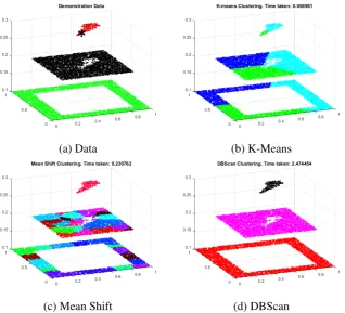
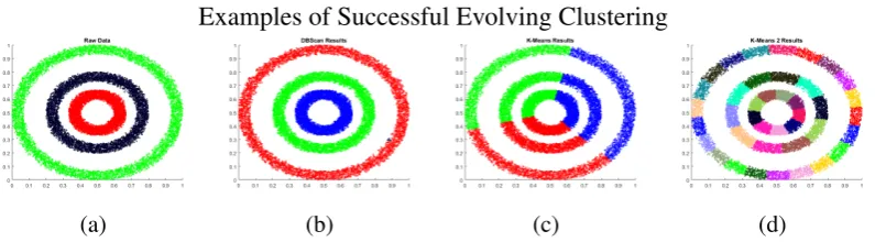
coun-tryside, black urban area and red is pollution release from the location identified by the asterisk. Pollution levels are 0.1, 0.2 and 0.3 respectively. Typical results from clustering techniques are shown in the remaining images. K-Means (b) is unable to create meaningful results when asked to find 3 clusters. We also see that distance based techniques such as Mean Shift (c), resulting in hyper-elliptical clusters, may identify the pollution but the larger regions are broken up and disjointed making it hard to visualise. This is a result of these types of techniques filling non-hyper-elliptical shapes with partial hyper-ellipses. In simple cases such as this it is possible to tune the radii along each axis such that each hyper-ellipse could be 'flat' to improve the results, however this requires a priori knowledge of the resultant cluster shapes. Arbitrarily shaped cluster resulting from techniques such as DBScan (d) produce arbitrarily shaped clusters which identify the regions with much greater accuracy. . 20 3.2 Example datasets used to illustrate clustering techniques. (3.2a) consists

(13)

has produced linkages 'across the gap' resulting in voronoi tessellations where the clusters meet . . . 24 3.4 (3.4a) shows the results of K-Means successfully clustering the Gaussian

data. (3.4b) shows how the random seeding of the K-Means algorithm can produce erroneous results. (3.4c) shows the results on the Spiral dataset demonstrating the limitations of hyper-elliptical, distance based clustering. The clusters actually form straight edges as they butt up against each other. . . 25 3.5 (3.5a) shows the results of Gaussian Mixed Models (GMM) successfully

clustering the Gaussian data. (3.5b) shows how the GMMs algorithm can produce erroneous results using the same parameters and data set. Gaussian Mixture Models are unable to cluster arbitrary, non-gaussian shaped clusters such as the spiral data set. . . 26 3.6 (3.6a) shows the results of DBScan successfully clustering the Gaussian

data, however, to separate the clusters low density portions of each cluster are identified as outliers. (3.6b) shows the results of reducing the minimum density to reduce the number of outliers has also merged two clusters. (3.6c) shows DBScan successfully clustering the spiral data set. All data not within a spiral is identified as an outlier. . . 27 3.7 (3.7a) shows the results of SubClu successfully clustering the Gaussian

(14)

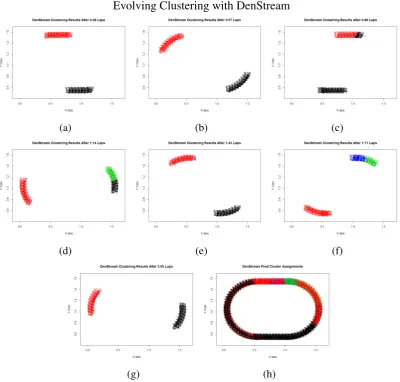
join that cluster. DEC does not have a limit for the cluster radius and so they continue to grow until they meet. At this time the people from one cluster move into the other cluster. . . 30 3.9 Plots of DenStream clustering of the two clusters moving around the race

track. With a value ofε=0.1 at some times the clusters are divided, 3.9c,

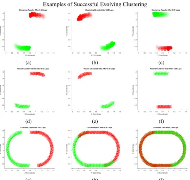
3.9d, 3.9f giving rise to the overall assignments shown in 3.9h. While not perfect, the clustering creates a more temporally accurate result than the Dynamic clustering. . . 31 3.10 Plots of various types of clustering results for fully evolving clustering.

The top row shows the data space occupied by the cluster definitions with the transparency proportional to the age of the data. The second row shows the recent data, within the decay period. Row three shows the final cluster assignment of the data. The red and green clusters are inter-mingled showing how the separate clusters have occupied the same data space at different times. Fully evolving clustering can ensure that the data is correctly assigned to the same cluster over time. . . 32 3.11 Example of clustering results on arbitrarily shaped natural clusters.

DB-Scan (3.11b) most closely matches the natural clusters, K-Means with k=3 (3.11c) is very poor, while K-Means with k=40 (3.11d) divides the natural clusters excessively. . . 41 4.1 Visualizations of the discussion in Subsection 4.2.3. Figure 4.1a shows

(15)

the most awkward shapes, Figure 4.2e . . . 48 4.3 Visualizations of the discussion in Subsection 4.2.4. Figure 4.3a shows

K-Means successfully clustering the Gaussian data, however this proved unreliable and frequently gave results as seen in 4.3b. Figure 4.3c shows K-Means is unable to make any sense of arbitrarily shaped clusters. Figure 4.3d shows DBScan successfully finding the Gaussian natural clusters, however a large number of outliers results form the high density required to prevent merging. DBScan excels at clustering arbitrary shaped data, Figure 4.3e, where the cluster quality more than outweighs the time penalty. . . 49 4.4 Visualizations of the Individual Household Electric Power Consumption

(16)

we can see the larger drop as we leave the central cluster. To avoid the radii estimation being triggered by in-cluster variations we smooth the data density drops as shown in Figure 4.5e. Where the density drop crosses the mean we can choose either the data sample before, or after the crossing point to give two option of radii which are shown in Figure 4.5f. . . 56 4.6 Visualizations of the DDCAR test results shown in Table 4.4. Figures

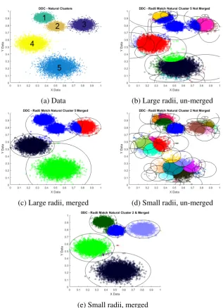
4.6a and 4.6b show similar results to those of DDC with manual radii entry. Figure 4.6c is generally quite good, however the merging function has combined two natural clusters in close proximity. Figure 4.6d show the un-merged clusters have not combined the two natural cluster demon-strating that the merge function is the root cause of this error. Figure 4.6e again indicates the errors introduced by the merge function where 4.6f shows the un-merged clusters proving reasonable results, albeit with a high number of clusters. . . 59 4.7 Testing the effects of the smoothing factor on DDCAR. Figure 4.7a shows

how the estimated radii are stable across a wide range of smoothing factor. Figure 4.7b shows the resulting accuracy of the clustering. . . 60 4.8 Testing the effects of the smoothing factor on DDCAR. Figure 4.7a

shows how the estimated radii are fairly stable across a wide range of smoothing factor. Figure 4.7b shows the resulting accuracy of the clustering. . . 62 4.9 Images relating to Subsection 4.3.5. Figure 4.9a shows the flight path

(17)

shows the raw data sets coloured by class. Figures 4.11f to 4.11f show the clustering results for DDCAS while Figures 4.11g to 4.11i show the results for DBScan. For a detailed analysis see Table 4.6. . . 69 4.12 Image for the DDCASmCplots. The Figures show plots of themConly

which clearly summarises the data locations with less information. . . . 70 4.13 Results of DDCAS clustering at 3 different times during the SAMBBA

B735 flight. The dashed black ellipse indicates the bounding region of the red cluster were it grouped by an elliptical distance based technique. By the third time period in Figures 4.13a, 4.13e and 4.13i the green anomalous data would not have been visible were it not for the arbitrarily shaped cluster definitions of DDCAS. . . 71 5.1 Illustration of kernel micro-cluster regions showing 5.1a micro-cluster

radius in magenta and, cluster kernel radius in blue 5.1b micro-clusters combined to the macro-micro-clusters, the grey shaded micro-cluster kernel did not overlap another micro-cluster and so is not included in the macro-cluster. . . 79 5.2 Figure 5.2a plots the run times for various techniques on higher

di-mensional data. Only ELM compares favourably, but it is limited to hyper-elliptical clusters only. Figure 5.2b shows the cluster results of CODAS projected back onto the x-y plane. Each coloured cluster is separated across 92 dimensions. . . 84 5.3 These plots show the different clusters formed, after the same number of

samples, for different, randomised, order of data. The cluster purity and accuracy are the same in all cases. . . 85 5.4 These plots show the different clusters formed, after the same number of

(18)

results with radius equal to the minimum gap between the clusters, Figure 5.6c shows the results of having a larger radius than the minimum gap and Figure 5.6d shows the effect of a much smaller radius. Thus radius is set by the user and should be less than the maximum dis-similarity data can have and still be considered a part of the same cluster. . . 92 5.7 Illustration of the Mackey-Glass data sets, a) the chaotic path b) the data

stream created around that path. The two Mackey-Glass streams are shown in red and green. When considering the data over the previous 'N

' samples the data may form separate streams, two clusters, or streams that are joined at some point, a single cluster. . . 96 5.8 CEDAS Auto Change Detection, changes in colour represent changes

in the number of clusters. Thus in figure 5.8a while the data is coloured green previous 'N' samples form a single cluster, joined at the beginning. At the point the data colour changes to black, the data in the previous 'N ' samples has separated into two clusters. It should be noted that the colours of the data are not the clusters themselves, but represent the time periods during which the data forms different numbers of clusters. The changes detected without noise are also detected with noise with the additional changes caused by temporary separate micro-clusters before they rejoin the main clusters. . . 98 5.9 Plot of mean processing time per sample in seconds for varying data

dimensionality. Each line represents the processing time for different decay periods which create a proportional increase in micro-clusters, e.g. the top, red line represents the processing time per sample for a decay period of 2,500 samples for data with dimensions from 1 to 5,000. . . . 100 5.10 Comparison of the processing time per sample with the decay time

(19)

5.12 (a) Plot of mean cluster purity (taken from [155]), (b) Mean cluster purity for CEDAS by the same measure as Wan et al. [155]. (c) Cluster purity at each time step showing instances of reduced mean purity. (d) CEDAS accuracy measure. . . 104 5.13 Figure 5.13a shows plots of the processing for MR-Stream for various

grid depths (from [155]). Figure 5.13b show the processing time for CEDAS to the same scale. . . 105 5.14 Plot of the number of classes of attack and the number of clusters found

by CEDAS in each time period. The number of clusters is proportional to the number of classes throughout. . . 106 5.15 Plot of the number of nodes or micro-clusters, which equates to memory

use, for MR-Stream (from [155]), DenStream and CEDAS. CluStream is not shown as it uses a maximum number of micro-clusters set by the user. CEDAS shows the lowest memory use. . . 107 5.16 Sample plots of short term decay periods (a)-(c) and medium term decay

periods (d)-(f). The short term variations indicated in (a)-(c) show the data varies over different 7 day periods. The medium term variations in (d)-(f) show that the data over the 28 day periods is more consistent and disguises the 7-day variation. . . 109 5.17 Plots of CEDAS clustering for a 28 day decay period showing a variation

of the data spread at different dates during a single year. . . 110 5.18 Plots of CEDAS clustering with a 28 day decay period showing variation

of the data for March over a 5 year period. . . 111 6.1 RASCAL operating screen showing (1) trace plot, (2) map plot, (3)

online clustering and (4),(5) offline clustering. . . 116 6.2 Plots of the visualization of cluster stages for DDC and CODAS. In plots

(20)

in black on the trace plot. . . 127 6.4 Using selectable data-stream clustering to explore data streams. By

selecting suitable data streams from the drop down menus we can apply clustering to MVK-MACR and Acetaldehyde. The display shows that the two selected data regions, red and magenta, both have raised levels of MVK-MACR and Acetaldehyde. . . 129 6.5 Identification of Further Regions of Interest: RASCAL screen view

showing model data comparison where the regions in red and black indicate where the model prediction is incorrectly predicting dips inO3

and magenta where the model accurately predicted narrow spikes inO3 130

6.6 Clustering technique outputs of the B735 flight showing clustering of typical data. . . 133 6.7 Alpha hulls of the data assigned to the main cluster at the 3 stages of

B735 analysis. Stage 1 shows typical data, stage 2 is after identification of the first anomaly and stage 3 at the end of the flight after discovery of the second anomaly. The three techniques are overlaid in each plot to indicate the similarity. . . 133 F.1 RASCAL initialization screen showing (A) trace plot information, (B)

(21)

3.2 Examples of typical cluster definitions by algorithm basis. . . 22

3.3 Summary of Offline Cluster Algorithm Types. . . 35

3.4 Summary of Online Cluster Algorithm Types. . . 35

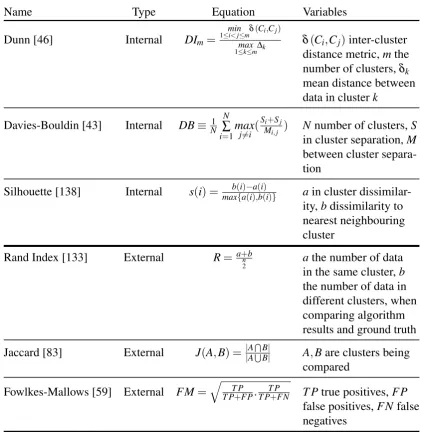
3.5 Common Cluster Quality Analysis Techniques . . . 39

[image:21.595.130.526.240.753.2]

3.6 Examples of cluster validity measures for the cluster results shown in Figure 3.11 . . . 41

4.1 Purity, Speed and Accuracy comparisons between DDC and alternative techniques. . . 51

4.2 DDC clustering results for various initial radii, on the Household Power dataset. . . 54

4.3 K-Means clustering results, for similar numbers of clusters to DDC, on Household Power dataset. . . 54

4.4 Purity, Speed and Accuracy for DDCAR. . . 60

4.5 Comparison of DDCAR Results with DDC. . . 63

4.6 Purity, Speed and Accuracy comparisons between DDCAS and DBScan. 69 4.7 Summary of offline clustering techniques used to meet the defined atmo-spheric science challenges. . . 73

5.1 CODAS Dimension Test Example . . . 82

5.2 Multi-Dimensional Speed Test Results . . . 83

5.3 CODAS synthetic data set test results. . . 84

5.4 Values foraandbused to solve the Mackey-Glass equations for the test data streams. . . 96

(22)

(23)

(24)

µ0 Global Mean: a term used in RDE calculations, the mean of all data samples in a

data set

µl the local mean of data samples

δ Mean density drop: a term used in DDCAR, the mean density drop between

adjacent data samples

{Cj} The set of data assigned to cluster j {Data} The set of data

al pha hulls a method for drawing around data points that allows for concavity where convex hulls do not

C_µ(i) CODAS mean of the data assigned to micro-clusteri, used as the centre

Ci(Centre) CEDAS, the centre of micro-clusteri

Ci(Count) CEDAS, the number of data assigned to micro-clusteri

C_i(Edge) CEDAS, the graph edges of micro-clusteri

C_i(Macro) CEDAS, the macro-cluster assignment of micro-clusteri C_m(i) CODAS macro-cluster assignment of micro-clusteri

C_n(i) CODAS number of data samples assigned to micro-clusteri

(25)

of data the clustering technique has defined as similar.

mC micro-cluster - small clusters of data limited to a local data space region, agglom-erations of which form macro-clusters

N Numeric count, specified locally in the text

n generic count specified locally in the text

natural cluster the clusters that are naturally present in the original data, which may differ from those found by a clustering technique.

O(D) Complexity notation based on the number of data dimensionsD O(n) Complexity notation based on the number of samplesn

r₀ initial radius for forming clusters, or micro-clusters

subspace where the full data space containsDdimensions, then a subspace is any part of that data space withndimensions where 1≤n<D

T_min minimum threshold for a micro-cluster to be considered part of a cluster rather than a group of outlier or noise data

X₀ Scalar Product: a term used in RDE calculations

x_{i j} clustered data sampleiin cluster j x_i un-clustered data samplei

(26)

1.1 Aims and Objectives

The role of atmospheric science, the data, its analysis and models has achieved great importance in recent times. Climate change and the future effect on Earth and its future has focussed much attention on research in this area. There is an on-going, increasing level of data gathering missions, both airborne and ground based which is resulting in an ever increasing amount of data to be analysed. Research in this area to date has generated numerous climate models which are extremely good at predicting typical climate changes. However, many have weaknesses when anomalous climate behaviour occurs. This thesis considers that one of the reasons behind this may be the data collection methods used. Typically these involve working with atmospheric sensors, whether mobile of stationary, in specific regions where it is predicted that data gathered will be of most use and add value to the models. The limited flight times, and pre-determined flight plans may result in fewer anomalous data being collected and limiting the input of anomalies to the models.

The aim of the research presented here is to investigate data analysis techniques to aid the collection, and analysis, of data gathered during these missions. The work comprises two key objectives:

(27)

Requirements for clustering analysis are proposed and current techniques investigated for suitability. The specifications are not easily matched, if at all, by current techniques and so new clustering algorithms are required. These are developed in both online and offline compatible modes. The algorithms are demonstrated and shown to have the potential to add value to data gathering missions, offline analysis and ongoing online analysis of atmospheric data streams.

1.2 Thesis Structure

The thesis is presented in separate Chapters, beginning with the Aims, Objectives and Thesis Structure provided in Chapter 1. Chapter 2 which presents an overview of Atmospheric Science and the source of the challenges to be addressed. There follows a review of current clustering and cluster evaluation techniques in Chapter 3 which considers how clustering could aid in addressing these challenges and where a summary of the key types of clustering that may be applicable is presented. Also discussed are the benefits and limitations of the generic types, and specific clustering techniques, summarising why they are not suitable for the final solution envisaged here. The offline techniques developed for this thesis are presented in Chapter 4 where the development of the preferred algorithms are detailed. The aim of the offline techniques is to develop suitable offline clustering techniques to allow compatibility in visualization and operation between offline and online clustering. Chapter 5 develops the online clustering algorithms which are key to the final online software solution for use by atmospheric scientists, RASCAL, which is presented in Chapter 6. RASCAL demonstrates how the techniques can be used in the field to enhance data gathering campaigns. Chapter 6 also briefly discusses an offline version of RASCAL which allows rapid reproduction of similar results to the online version. A number of improvements to the online version, based on feedback from the Atmospheric Science community, have been included in the offline version.

(28)

(29)

outline the basic physics of climate change, the resulting economic and health costs, and outline the role of atmospheric science and its funding in the scientific analysis of climate change in Section 2.2. Section 2.3 describes the characteristics of a typical atmospheric science data gathering campaign and the type and size of data sets such campaigns produce. Finally Section 2.4 outlines the challenges to be addressed during this research.

2.1 The Atmosphere of Earth

As the world has come to accept the reality of Climate Change and its current and future impact on the world the importance of the scientific study of the changes and their effects has become ever more significant. The atmosphere surrounding the Earth has significant impact on the global temperatures and the composition of the air that we breathe. The complex interaction of the chemistry in the various atmospheric layers determine the radiation reaching and leaving the Earth’s surface, the temperatures of the atmospheric layers (Global Warming) and the dispersion of pollutants.

The Earth’s atmosphere comprises a mixture of gasses surrounding the planet with most common being Nitrogen (N₂) at 78%, Oxygen(O₂) at 21% and various others at less than 1% including Carbon Dioxide(CO₂). Water vapour is also present at varying levels and also small particles known as 'aerosol particles' from various sources both natural and anthropogenic [152].

(30)

temperature with height due to the absorption of solar radiation.

3. Mesosphere (50-85km) is difficult to study as it lies above the heights reachable by aircraft or balloon, but below that of orbital satellites.

4. Stratosphere (10-50km) A temperature inversion appears again here due to the ab-sorption of solar radiation by Ozone (O3) which is relatively abundant (i.e., several

to a few tens of molecules of ozone per million molecules of air - parts per million (ppm)). The lack of vertical convection within the stratosphere, and between the stratosphere and Troposphere, means that air that reaches the stratosphere may remain years or even decades [113, 146]. Air moving into the stratosphere carries with it chemicals such as CFCs (chlorofluorocarbons) which have a significant impact on the ozone levels.

5. Troposphere (0-10km) contains most of the mass of the Earth’s atmosphere. Char-acteristically the temperature drops as the height increases but layers with constant or increasing temperature with height are not uncommon. Most cloud formations appear in the troposphere and nearly all weather phenomenon occur here.

6. The Planetary Boundary Layer is the lowest part of the troposphere and is in contact with the Earth’s surface. This contact allows the surface to affect the atmosphere - through exchange of heat, momentum, gases, and particles - and so some atmospheric behaviour is directly influenced by that contact.

In addition to the primary layers there are boundary regions between them. These boundaries play an important role, affecting the movement of air between the layers. They are a focus of study for atmospheric scientists, particularly the chemistry transport across these boundaries and the effects on the primary layers. These boundaries are:

1. Thermopause, the boundary between the thermosphere and the exosphere 2. Mesopause, the boundary between mesosphere and thermosphere.

(31)

The atmospheric layers being considered in this thesis are primarily the Boundary Layer, Troposphere and Stratosphere together with the tropopause. The Coordinated Airborne Studies in the Tropics (CAST) project, of which this research is a part, was specifically targeted to investigate the interactions between these layers in a coordinated effort to study the atmospheric chemistry and transport between these layers [75].

2.2 Climate Change

Climate change is now considered an accepted theory with far reaching effects. These effects will vary globally with a range of economic, social and health impacts. The Projection of Economic impacts of climate change in Sectors of the European Union based on bottom-up Analysis (PESETA) project report [34] considers many aspects of possible climate change scenarios across the EEA including he effects on agriculture, coastal systems, river floods, tourism and health. The findings indicate and annual cost to the EEA economy to be C20 to C65 billion between scenarios of 2.5oCand 5.4oC

temperature rises.

2.2.1 Economic Costs

(32)

is predicted to be an increase in heat related mortality balanced by a decrease in cold mortalities. The PESETA report also indicates a potential cost of several Billion Euro associated with climate sensitive diseases, allergens and air quality.

2.2.3 The Role of Atmospheric Science

Atmospheric Science has a key role to play in the study of climate change. The Earth’s atmosphere is a significant part of the global climate and the uptake, transport and deposition of chemicals and pollutants all have an impact, generating an ever growing body of research e.g. [24, 31, 151, 73, 60, 38, 76]. The models used to predict the various scenarios rely on accurate input data and the accuracy of their predictions can be tested with subsequent monitoring. Such is the importance of these climate models that comparing the models are constantly compared, evaluated, modified and updated [94, 91, 21, 11, 79, 12].

With the wide range of potential costs and impact of the modelled scenarios the importance of atmospheric science in the role of climate science is apparent. The uncertainties involved in modelling such complex dynamical systems and the sensitivity to small changes, 'The Butterfly Effect', underline the importance of accurate data. Data from anomalous events can be of particular interest to adjust models to predict such unusual, or extreme, events, or to be ignored as genuine 'anomalies' which may be considered unpredictable.

2.2.4 Climate Science Funding

(33)

IPPC report on climate change [147]). Process-based models fill-in data-gaps (e.g. the ERA re-analysis project [54]), diagnose probable causes of observed events (e.g. extreme events like the Boscastle floods [69], or tropical hurricanes [112]), and provide forecasts of future weather, climate, and atmospheric composition. Most atmospheric observations are made operationally at a network of ground stations, or using satellites. However, to diagnose atmospheric processes in more detail than is possible using operational observa-tions, intensive field campaigns are used. Atmospheric science campaigns typically run over days, weeks or longer and involve a number of possible sources of data. The include instruments on board aircraft, ground based instruments, rising sondes and drop-sondes. Additionally, there are continuous data streams from the standard aircraft instrumentation providing non-chemistry data such as aircraft position and status. Here we will describe two example atmospheric science campaigns.

The South AMerican Biomass Burning Analysis (SAMBBA) [110] had specific objectives to study the pollution and effects of biomass burning in the South American rainforests. The main SAMBBA findings were reported in a special issue of Atmospheric Chemistry and Physics [7, 22, 92, 106, 126]. As with all such data sets research and publication is on-going. The SAMBBA campaign (Sept. - Oct. 2012) made use of the Facility for Airborne Atmospheric Measurements (FAAM) BAe-146 aircraft configured with 52 instruments on board [23]. The flight paths are shown in Figure 2.1a with each shown in a different colour. We will use the data from this campaign later in the thesis demonstrating specific example of how the results of this research can add value to these missions.

(34)

(a) SAMBBA Flight paths. (b) CAST Flight paths.

Fig. 2.1 Maps of the flights paths for 2.1a SAMBBA campaign and 2.1b the CAST campaign. The SAMBBA campaign focussed on higher altitudes up to approximately 8,000m, with some time spent at 1,000m-2,000m. CAST focussed on lower altitudes around 500m-1,500m with some time spent up to approximately 6,000m

.

full atmospheric range from ground to stratosphere three aircraft with complementing configurations of instruments on board flew at a range of heights.

• Low altitude sampling was carried out by the FAAM BAe-146 at heights between 0 - 6,000m

• Mid altitude flights were carried out by the NCAR GulfstreamV (GV) flying between 6,000m - 14,000m

• High altitude flights carried out by NASA’s Northrop Grumman Global Hawk UAV at altitudes up to 14,000m - 20,000m

These are the target flight altitudes, in practice there was some overlap between the aircraft flight profiles. The campaign took place in a 6 week period in January and February 2014 from bases around Guam in the Western Pacific.

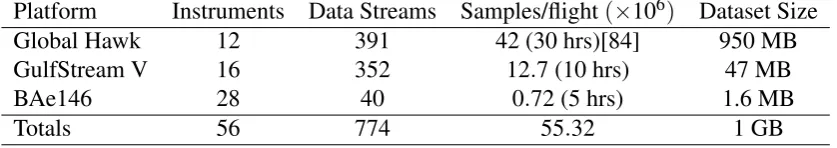
The instruments carried by the FAAM BAe-146 aircraft [120] are primarily self-contained and capture and store the data for download post-flight. Some instruments currently gather air samples for later analysis so the data is not available in flight. Final data is not provided until much later after instrument calibration and necessary adjustments have been made, although 'quicklook' data is often available in real time. In total there were 28 instruments, 35 including the standard core instrumentation and basic flight instrumentation.

(35)

of statistical bins. The total number of potential data streams is 352 in the instrument configuration deployed during the CAST project.

The NASA GH had a payload of 12 instruments [115] plus standard flight information. Some of the instruments provide chemistry information on multiple chemical species. Other instruments measure particle size or concentrations in different ranges. Taken as separate data sources and not including error flags there were a total of 391 data streams. As an unmanned vehicle the data from the GH is sent to the ground as data streams already although it is not processed online.

Typical examples of the volume of data gathered during campaign flights are given in table 2.1. These figures are based on a 1Hz sampling rate for a typical full flight duration. In practice flight durations may change and sample rates vary per instrument.

2.4 Atmospheric Science Data Challenges

With most data analysis occurring post-campaign, data pertaining to anomalies or other data of specific interest may be limited. Processing the data online and in-flight could improve the data collected by helping focus the data gathering on specific regions of interest. As discussed in Section 2.3 it can be seen from Table 2.1 that the volume of data captured and streamed to mission scientist is vast. Faced with this torrent of data it may often be the case that mission scientists focus on a small subset of the available data. New techniques and analysis are required to aid mission scientists by providing online analysis of the data to simplify the decision making process during campaigns. Additionally, these analysis techniques should be reproducible offline for post-campaign analysis and re-analysis of historical data.

[image:35.595.108.527.155.229.2]

(36)

1. Differing y-axis scales for multiple plots. Providing a single plot window for multiple data streams may result in a range of y-axis maximum values. The resulting plot can be confusing with either multiple y-axis scales, or, in extreme cases, featureless horizontal plot lines at the top and bottom of the graph.

2. Sizes of plot markers. Plot marker size can have a noticeable affect on data visualization. Large plot marker sizes may hide new data points or give the appearance of merged regions of data. Small markers may be hard to see and to distinguish between colours in colour plots.

3. Visualization of historical data. Line plots may be of limited use for extended time scales. As the data gets compressed into the plot window fine details of anomalies or 'spikes' may be hard to see, and may even not be present. Scatter plots suffer from the marker size problem mentioned above.

4. Distinguishing colours or markers. There are limits to the numbers of colours it is possible to distinguish by the human eye, particularly with many lines, or markers overlapping.

5. Over plotting of similar data. Both line plots and scatter plots suffer from overwrit-ing of old data such that the latest line to be drawn, or data to be plotted, overwrites and obscure underlying information.

2.4.2 Discrete Data Sampling

Although data may be continuous, discrete sampling rates result in point data rather than data space regions of similar values. This produces line or scatter plots as described in Section 2.4.1 and datasets of discrete samples. The reality is continuously variable data such that a small change in sample time and, therefore spatial location, would produce a similar, but slightly different, reading.

2.4.3 Online Chemistry Analysis

(37)

and 'global' anomalies. Local anomalies refer to data that is anomalous over a specific range, typically a temporal range, although the data may not be unusual in general, e.g. a temperature of 18oCis rather anomalous for December in the UK, but is quite normal for summer. To continue that example, a temperature of 35oCwould be considered a 'global' anomaly as it is an unusually high temperature for the UK at any time of year.

It is therefore necessary to differentiate data drift, gradual expected changes, from data anomalies. Such temporal separation may be important for the understanding of pollution which may have both diurnal and seasonal variation [134].

2.4.5 Online Identification of Drift

As mentioned in the previous Section, 2.4.4, differentiating between drift and anomalies may be important. This is not only true for the identification of anomalies, but also for identifying general drift and in readings which may be important in themselves. To continue the example from the previous Subsection it may be significant to notice general drift in the UK temperature for a given month over several years and to notice that the drift is independent of any anomalies. However this can equally apply to spatial drift during flight operations, e.g. moving over different terrain types, or from land to ocean areas.

2.4.6 Historical and Temporal Separation of Chemistry

(38)

on shifts to cover the full duration of the flight. When new operatives start their shift presenting them with historical analysis of the flight up to that time is useful to aid understanding of the data captured. With historical analysis available it is also possible to compare previous flight data from the campaign, or even data from previous campaigns. The same reasoning can be applied to data streams gathered over many years and across many data missions.

2.4.8 In Flight Analysis for Flight Path Adaptation

During many data science campaigns the data found is broadly consistent with that expected and predicted by weather, climate, or operational pollution forecast models. In some cases, however, it may be found that significant anomalies are discovered during post campaign analysis, whether they be anomalous to typical data gathered so far, variations from predicted model output values or the data specific to the main investigation of the campaign, such as evidence of biomass burning [143]. Identifying such data in-flight would enable potential changes to the flight path to capture more of the anomalous data. This additional data may be of significance in either improving climate models, providing additional data for the primary investigation or identifying unexpected chemistry.

2.4.9 Rapid Future Flight Planning

Similar to the way that online analysis can aid in flight route changes, the same can be said for future flight plans. The on-line information available during a flight, together with the ability to reproduce the analysis post-flight could provide a useful insight into the geographical locations of the data of most interest. This information can feed in to the future flight plans.

2.4.10 Reproducible Analysis Post Sortie

(39)

1. Data Collection Improvement by online analysis and identification of data of interest allowing targeting specific spatial locations providing the most appropriate data.

2. Online Data Analysis challenges to provide the insight necessary to help improve the data collection.

3. Post Flight Analysis to reproduce the online analysis when applied to the full flight dataset.

(40)

Quality Measures

This chapter provides a summary of how clustering techniques could aid in responding to the Environment Science data challenges proposed in Chapter 2.4. Each challenge is introduced in Section 3.2 with an overview of how clustering may help and what type of clustering may be best suited to address each challenge. Current clustering techniques are discussed in Chapter 3.3 with Sections devoted to: the advantages of hyper-elliptical versus arbitrarily-shaped clusters, 3.3.1; offline techniques, 3.3.2; online techniques, 3.3.3; and the compatibility between the two, 3.3.5.

(41)

should be more similar to data within its cluster than to data in other clusters. Many early techniques required a priori knowledge of the number of clusters to be found. Later developments found other methods of generating the clusters with different user inputs, e.g. the typical expected size of a cluster in the data space. These early techniques, and this cluster definition has significant limitations as to they type of data groups that could be found, very early techniques discovering hyper-spherical clusters, later methods extending this to hyper-elliptical clusters. Yet, groups recognisable by humans vary con-siderably from these simple shapes and later developments allowed the discovery of data groups of arbitrary shapes. Another development path for clustering algorithms moved the techniques from the offline realm, where all data is available, to online techniques where data streams constantly update the available data leading to 'online' and 'evolving' techniques. These different techniques are discussed in the following Subsections.

(42)

These form the requirements of the techniques and they are summarised in Table 3.1. 1. Improving the Visualization of Online Data Streams. Clustering techniques

can be used to display the data space regions in which the data has appeared, not just the exact data points measured. This can be achieved by clustering the data and/ or using alpha hulls or similar to outline the data region. This requires extra processing beyond the original clustering technique and this additional process needs to be repeated with every data sample.

When a single data stream is chosen for visualization from the start then the technique can be independent of offline techniques. However, if it is expected that a change of data streams may be warranted for any reason then the clustering technique should be compatible with an offline clustering technique. In this way the historical data can be clustered offline before the online method takes over and updates continuously from that time.

2. Online Anomaly Detectionrequires an online clustering technique that allows for drift in the data, yet still displays local anomaly changes. Anomalous data could expand hyper-elliptical cluster shapes, yet still leave much of the data space within that cluster empty of data samples. It is possible that new anomalies may go unnoticed should they appear within that empty cluster space. To avoid this the cluster shape should accurately cover the recorded data only, i.e. must generate arbitrarily shaped clusters. Again, as outlined in 1, the techniques should be compatible with an offline technique.

(43)

fast, as the historical datasets may be large. When applying the offline clustering techniques it is important to ensure that the clusters, and data space regions in which they lie, are consistent with any online technique. This ensures that the visualizations created are consistent.

6. In Flight Analysis for Flight Path Modification. In flight cluster analysis re-quires an online clustering technique. As outlined before it is important that the technique is capable of producing arbitrary shapes and responding promptly to anomaly detection.

7. Rapid Future Flight Planning. Future flight planning can benefit from the results of any online, in-flight clustering, or from reproducing the analysis offline with more detailed investigations. The clustering results may add information regarding the locations of data that is of most interest.

8. Reproducible Analysis Offline, Post Sortie and Post Campaign. Reproducing any online in-flight analysis offline will allow for more detailed examination of data. In flight the main user of the analysis is likely to be the mission scientists, however offline any experts can be easily involved in examining the data, analysing and identifying data of interest.

3.3 Current Clustering Techniques

This section will discuss the techniques, and resulting clustering, of current clustering techniques. Based on the responses to atmospheric science challenges many alternative clustering techniques will be considered and their suitability assessed. Visualizations are included as an aid to understanding the text. The clustering results they show are not intended to indicate the best, or worst, possible result of any technique, but merely to give clarity to the text.

(44)

2 Y Y Y Y

3 Y Y Y Y

4 Y Y Y

5 Y Y Y

6 Y Y Y Y

7 Y Y Y

8 Y Y Y Y

3.3.3, an examination of hyper-elliptical and arbitrarily shaped clusters in online, dy-namic and evolving clustering techniques where different challenges arise from those of offline techniques. Subsection 3.3.5 reviews the typical results obtained from the offline techniques and discusses their compatibility with online techniques. Finally we summarise the techniques and consider a path for applying clustering to the atmospheric science challenges in Subsection 3.3.6.

3.3.1 Elliptical Versus Arbitrarily Shaped Clusters

Clustering can be grouped into two main types, those that use a purely distance based measure and produce hyper-elliptical clusters (in terms of the distance measure used), or those that use density-linked type groupings that produce arbitrarily shaped clusters. It is acknowledged that where hyper-elliptical cluster encroach on each other’s data space they may form centroidal voronoi tessellations but throughout this thesis they shall be referred to as hyper-elliptical clusters and techniques in reference to their cluster membership functions.

(45)

(a) Data (b) K-Means

[image:45.595.159.478.184.473.2]

(c) Mean Shift (d) DBScan

(46)

In practice clusters such as those shown in Figure 3.1 result. Artificial data comprising of 10,000 data samples is used to represent a typical pollution based scenario as shown in Figure 3.1a. 'Countryside' is represented by the green data, with a pollution level of 0.1. The black region represents an 'urban' region with pollution levels of 0.2, while the red data represents a specific 'pollution' release with pollution levels of 0.3. The data represents a time after the start of the pollution release where the pollution has drifted and spread somewhat. We can see from these plots that, despite its popularity in atmospheric science, k-means is unable to create meaningful clusters from the data and k-medoids produces similar results, Figure 3.1b. Mean shift is capable of separating out the small pollution region, but the urban and countryside regions are broken up into multiple clusters, Figure 3.1c. This is an improvement over analysing the raw data, as we have fewer groups of data, which we have identified as similar. However, when using arbitrarily shaped cluster techniques such as DBScan, we can see that the each of the different regions can be clearly identified, Figure 3.1d.

It is worth clarifying that in many cases density based clustering techniques fall in to the group of distance based techniques and, so, tend to produce clusters of hyper-elliptical shapes. This is not necessarily the case however, it is just that many density calculations are themselves distance based. There are, of course, situations where hyper-elliptical techniques may be more appropriate to use. If the data is known to be, or can be approximated to, hyper-ellipses then the speed of the hyper-elliptical techniques may be of considerable advantage. Even on the simple example, shown above, of 10,000 samples of 3 dimensional data we see an approximately 10 fold reduction in clustering time between DBScan at 2.47s and Mean Shift at 0.23s.

Both distance-based and density-linked arbitrarily shaped clustering techniques are considered throughout this thesis to compare the differences and trade-off between accurate data representation and speed.

3.3.2 Offline Clustering Techniques

(47)

Distribution Data belonging to a cluster should most closely form a pre-defined statistical distribution

Density Data belonging to a cluster should be connected to all other data in the cluster by regions of a defined density range.

Sub-Space Data may belong to multiple clusters in multiple sub-spaces. The number of subspaces is 2d for orthogonal sub-spaces and infinite for non-axis-parallel. Any clustering algorithm is possible within the subspaces.

similarity. Clusters do not have a single definition and different clustering techniques may use different definitions to suit their algorithms. Examples of cluster definitions are given in Table 3.2.

The aim of offline clustering is typically to produce a list of cluster assignations, or cluster membership likelihoods, for each data sample. In this way the definition of each cluster may be a large and unwieldy vector list. Cluster results consisting of a full data sample list are particularly problematic when interfacing with online techniques.

One of the key drivers of online techniques is memory and computational efficiency, especially for on-going, endless data streams. Storage of the full data stream will require enormous memory capacity. Additionally, comparing future incoming data to that already stored will require ever increasing processing time. The next section will discuss on-line clustering techniques in detail, however it is clear that the results produced by traditional offline techniques are not directly compatible. Offline clustering results could, possibly, be converted to a compatible format by grouping and analysing the results with an interface algorithm. However, this is generally an offline, compatible version of an online algorithm and will also require additional processing time.

(48)

(a) Gaussian Data (b) Spiral Data without Noise (c) Spiral Data with Noise

Fig. 3.2 Example datasets used to illustrate clustering techniques. (3.2a) consists of 5 clusters of Gaussian distributed data. (3.2b) consists of 3 spirals of data, with no noise. (3.2c) consists of the same spirals but with random noise across the data space.

Connectivity Clustering

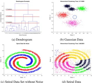
Connectivity based cluster analysis refers to techniques such as Hierarchical clustering [109] and developments of this technique. It has two forms, 'agglomerative' and 'divisive'. In agglomerative analysis all the data samples are considered separate clusters initially and are merged, based on an appropriate distance measure, until only one cluster remains. The results are often presented in a dendrogram to allow the user to decide the appropriate cluster split, however, this can be automated to suit a user input for the number of clusters, or a pre-determined linkage height. Divisive analysis functions in reverse with the initial state being a single cluster, which is then divided until all data samples are separate.

Typical results for Hierarchical clustering are shown in Figure 3.3 which show the limitations of the technique. Under certain circumstance Hierarchical clustering is capable of producing some arbitrarily shaped clusters, e.g. where cluster are well separated with little or no noise as shown in Figures 3.3b and 3.3c. However, noisy data can create linkages between natural clusters as seen in Figure 3.3d. Hierarchical clustering has complexity ofO(n3)for agglomerative andO(2n)for divisive clustering with exhaustive search. This high complexity, combined with high memory requirements, makes it unsuitable for large datasets even with optimised algorithms such as SLINK [140] or CLINK [44].

Centroid Clustering

(49)

(a) Dendrogram (b) Gaussian Data

[image:49.595.156.471.100.386.2]

(c) Spiral Data Set without Noise (d) Spiral Data

Fig. 3.3 Typical agglomerative analysis dendrogram (3.3a) based on the Gaussian sample data indicating linkage heights for 2, 3 and 5 clusters. (3.3b) shows the results on the Gaussian data. Outliers on the magenta cluster (circled) have distorted the results causing 2 clusters to merge (black) and preventing the successful identification of the 5 clusters. Figure 3.3c shows successful clustering of arbitrary shapes where no noise is present. Figure (3.3d) shows the results on the Spiral dataset where noise has produced linkages 'across the gap' resulting in voronoi tessellations where the clusters meet

to a single cluster. However, fuzzy techniques are also available where each data sample is a assigned a membership likelihood for each available cluster.

(50)

(a) Gaussian Data Clustered Well

(b) Gaussian Data with Erroneous Clustering

(c) Spiral Data is unsuitable for K-Means

Fig. 3.4 (3.4a) shows the results of K-Means successfully clustering the Gaussian data. (3.4b) shows how the random seeding of the K-Means algorithm can produce erroneous results. (3.4c) shows the results on the Spiral dataset demonstrating the limitations of hyper-elliptical, distance based clustering. The clusters actually form straight edges as they butt up against each other.

drawback. Fuzzy-C-means [19] is similar in principle to k-means, however, each data sample is given a 'membership' value for each cluster, rather than being assigned to a single cluster. Figure 3.4 illustrates some of the short comings of k-means, and other typical centroid clustering algorithms.

Subtractive clustering, a technique based on mountain clustering [163], does not require the number of clusters to be predetermined. Rather it uses a radius, within which to include data samples in the cluster. The centroid of the cluster is calculated by determining which data sample has the minimum distance to all other data samples. This data sample and all those within the user-defined radius are considered to be a cluster and are removed from the data set. The process is repeated until all the data is clustered. With appropriate radii the technique can discover the correct number of clusters, however it is susceptible to incorrect radii, i.e. too small a radii and natural clusters will be broken into smaller clusters, too large a radii and natural clusters may merge.

Distribution Clustering

(51)

(a) Gaussian Data Clustered Well (b) Gaussian Data with Errors

Fig. 3.5 (3.5a) shows the results of Gaussian Mixed Models (GMM) successfully cluster-ing the Gaussian data. (3.5b) shows how the GMMs algorithm can produce erroneous results using the same parameters and data set. Gaussian Mixture Models are unable to cluster arbitrary, non-gaussian shaped clusters such as the spiral data set.

k-means the a priori knowledge required to define the number of Gaussian distributions is a limiting factor. Examples of the limitations of GMMs are shown in Figure 3.5.

Density Clustering

Density based clustering refers to techniques that cluster data based on similarity of data density. The most well known of these techniques is DBScan [53]. DBScan has limitations in terms of complexity(O(n2)) and its inability to distinguish clusters of varying density. Many variations have been proposed to overcome these limitations such as hybrid techniques by Yasser et al. [49] which first uses CLARANS [123] to partition the data space. VDBScan [97] improves the speed of DBScan by first ordering the data and only visiting data samples outside of the radius defined byε, the density radius. A

critical analysis of most variants on DBScan can be found in Ali et al [6].

The demonstration data Gaussian distributions can be clustered as shown in Figure 3.6a, however, lower density regions of a cluster may be labelled as outliers. If the required density is reduced then lower density regions between clusters may cause them to merge as shown in Figure 3.6b. Density based clustering techniques are able to find cluster of arbitrary shapes as illustrated in Figure 3.6c. Note also that the time for clustering, as shown in the plot title, shows a significant increase over alternative methods illustrated in this chapter.

Subspace Clustering

(52)

(a) Gaussian Data with well separated clusters, but many

outliers.

(b) Gaussian Data with merged clusters and fewer outliers.

(c) Spiral Data with good clusters and outliers identified.

Fig. 3.6 (3.6a) shows the results of DBScan successfully clustering the Gaussian data, however, to separate the clusters low density portions of each cluster are identified as outliers. (3.6b) shows the results of reducing the minimum density to reduce the number of outliers has also merged two clusters. (3.6c) shows DBScan successfully clustering the spiral data set. All data not within a spiral is identified as an outlier.

the clusters in the full data space may not be of as much interest as those in certain sub-spaces, e.g. in gene expression mapping a certain gene may be associated with disease A in combination with one set of genes and disease B in combination with others. Or where such a dataset contains a value for 'age' this attribute may disperse the data so they do not form clusters if 'age' is not relevant to the diseases then clusters will only be present in a subspace if it does not include 'age'.

Subspace clustering falls into two broad groups: Top Down and Bottom up. Top down approaches such as PROCLUS [4] and FINDIT [159] find clusters in the full data space, then evaluate the subspaces of each cluster. Bottom up approaches such as Mafia [68], Clique [5], SubClu [88] and others find clusters in low dimensional subspaces, the lowest being each data axis, and combining them in higher dimensional subspaces to form higher dimensional clusters. A review of subspace clustering techniques can be found in [165, 128].

(53)

(a) Gaussian Data with well separated clusters, but many

outliers.

(b) Gaussian Data with merged clusters and fewer outliers.

(c) Spiral Data cannot be clustered.

Fig. 3.7 (3.7a) shows the results of SubClu successfully clustering the Gaussian data, however, to separate the clusters low density portions of each cluster are identified as outliers. (3.7b) shows the results of reducing the minimum density to reduce the number of outliers results in the merging of nearby clusters. (3.7c) illustrates a limitation of SubClu as each subspace consists of only a single cluster despite clearly separate groups.

3.3.3 Online, Dynamic and Evolving Clustering Terminology

(54)

discussed in this section this is achieved, not by dividing the clusters in an online manner, but rather by re-clustering using an offline clustering technique on demand. With ever-increasing data sets, i.e. 'Big Data', the need to discard or archive the data after processing once becomes necessary for both computational and memory efficiency.

Online clustering differs considerably from offline clustering. The aim of online clustering is to group data into clusters, as defined by Table 3.2, from streams of data. These streams of data may be open ended resulting in data sets that would be too large to remain in memory. The data can be discarded completely and / or archived for later use.

Data can be assigned to a cluster as they arrive, and these results stored along with the data. This, however, has inherent dangers. As clusters change, move and evolve over time the cluster assignment originally assigned to the data may no longer be correct at a later point in time. It is easily conceivable that two similar data samples could be assigned to separate clusters simply due to the temporal difference. In such a case it should be a matter of record that the cluster assignment was only correct at the time it was made.

As an alternative, the data space regions covered by the clusters could be evolving and, when the cluster assignation is required for any data they are checked with the current cluster status and the assignment made. In this way the cluster assignation is current and correct with the latest cluster state. This however has the complications in finding out the historical cluster assignation at the time the data sample was taken and it is possible that two data samples of similar values find themselves in the same cluster, when we would prefer them to be separate due to the temporal separation. It is important, therefore, to select the correct technique for the intended use of the data and clusters.

Online clustering techniques can be broadly categorised by the type and nature of the data streams they are operating on. There is no formal agreement on the terminology so this thesis uses perhaps the most common descriptive names for these different types: 'Dynamic Clustering' and 'Evolving Clustering'.

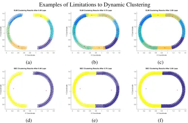
Dynamic Clustering

(55)

(a) (b) (c)

[image:55.595.120.509.94.349.2]

(d) (e) (f)

Fig. 3.8 Plots of clustering results for two dynamic clustering techniques, the top row is ELM, bottom row DEC, showing different techniques for dealing with unrestrained cluster growth. The plots show clustering of 2 groups of people running three laps of an oval track. ELM places a user-defined hard limit on the cluster radius resulting in multiple clusters. When people arrive at a location where data has previously been clustered, they join that cluster. DEC does not have a limit for the cluster radius and so they continue to grow until they meet. At this time the people from one cluster move into the other cluster.

their size and position to better group the data. In some cases clusters may merge as data arrives in the spaces between them. Dynamic clustering has no 'ageing' parameter and so clusters, once formed, remain indefinitely. In this thesis we will refer to data streams with such natural clusters as 'Dynamic Data Streams', i.e. as the natural clusters may move or change size, but are not analogous to biological evolution in that the clusters do not die and are not born into new generations. It doesn’t require much imagination to conceive of a situation in which the data space become completely full with both data and their respective clusters. This is particularly true of dynamic systems in which the data can vary across the full range of their respective limits.

(56)

(a) (b) (c)

(d) (e) (f)

[image:56.595.114.515.98.480.2]

(g) (h)

Fig. 3.9 Plots of DenStream clustering of the two clusters moving around the race track. With a value ofε=0.1 at some times the clusters are divided, 3.9c, 3.9d, 3.9f giving

rise to the overall assignments shown in 3.9h. While not perfect, the clustering creates a more temporally accurate result than the Dynamic clustering.

limitations in place to prevent this then either multiple clusters occur, Figures 3.8a-3.8c, or the clusters grow until they meet, Figures 3.8d-3.8f.

Evolving Clustering

(57)

(a) (b) (c)

(d) (e) (f)

[image:57.595.121.511.182.551.2]

(g) (h) (i)

(58)

3.10 where we see that the red and green clusters are traced as separate clusters, even when they occupy similar data space, due to the temporal difference of when they occupy that data space, i.e. all the green data is always associated with all other green data and never with the red data and vice versa.

Evolving data streams are particularly relevant in situations where historical data has a reduced effect on recent events. Such situations occur in financial transactions, machine condition monitoring and, of particular relevance here, environmental monitoring as discussed at the start of this chapter.

3.3.4 Online Clustering Techniques

Online clustering techniques fall into two main classes, 'single-stage' and 'multi-stage'. Single-stage techniques complete the cluster updates in a single pass as the data arrives whereas multi-stage techniques use (typically) a two step algorithm whereby 'micro-clusters' (mC) are updated online as the data arrives and 'macro-clusters' (MC) are created from agglomerations of these micro-clusters.

Single stage techniques are invariably distance based, producing hyper-spherical, or hyper-elliptical, clusters in the data space. ELM [47] and DEC [15] are both single stage techniques however they differ in their approach to limiting cluster growth. ELM uses a bandwidth parameter which limits the cluster radius to a maximum value resulting in the clusters shown in Figure 3.8a-3.8c. The data in each cluster is indeed similar to each other, however the arbitrary boundary may result in the division of natural clusters. DEC does have an ageing parameter which reduces the importance of old data and old clusters. However the clusters are not removed completely such that, if a recent data moves into the data space occupied by an old cluster, then the new data becomes part of the older cluster. Thus DEC is somewhat of a halfway stage between dynamic and evolving clustering.

(59)

regarding the number of expected clusters. ClusTree [93], DStream [32] and Denstream [26] make use of DBScan [53], while DSClu [114] uses a very similar approach, and so are capable of findingMCs of arbitrary shape.

The secondary, offline, stage is somewhat of a bottleneck for these techniques. While the online maintenance of the micro-clusters may be extremely fast the time penalty of the offline stage may limit the finalMCstage to being either periodic, or on demand.

3.3.5 Compatibility Between Offline and Online Techniques

For the proposed solutions of the Atmospheric Science challenges, in particular that outlined in Section 1 it is a requirement to find compatible offline and online clustering techniques. This will allow a fast offline technique to rapidly cluster historical data in such a way that allows an online technique to take the clustering results and continue. The inherent difference between offline and online techniques, i.e. offline results provide all the data with cluster assignment, whereas online techniques provide data space regions, means that offline and online techniques are not directly compatible. It would therefore be required to develop an interface between the methods, or to develop new techniques which are compatible.

The rest of this thesis presents the work carried out to create a suite of clustering techniques that satisfy all the criteria required of the Atmospheric Science challenges, together with the development software used to demonstrate the validity of the approaches in a data gathering mission environment.