Vehicle point of interest detection using in car data

warwick.ac.uk/lib-publications

Manuscript version: Author’s Accepted Manuscript

The version presented in WRAP is the author’s accepted manuscript and may differ from the

published version or Version of Record.

Persistent WRAP URL:

http://wrap.warwick.ac.uk/109183

How to cite:

Please refer to published version for the most recent bibliographic citation information.

If a published version is known of, the repository item page linked to above, will contain

details on accessing it.

Copyright and reuse:

The Warwick Research Archive Portal (WRAP) makes this work by researchers of the

University of Warwick available open access under the following conditions.

Copyright © and all moral rights to the version of the paper presented here belong to the

individual author(s) and/or other copyright owners. To the extent reasonable and

practicable the material made available in WRAP has been checked for eligibility before

being made available.

Copies of full items can be used for personal research or study, educational, or not-for-profit

purposes without prior permission or charge. Provided that the authors, title and full

bibliographic details are credited, a hyperlink and/or URL is given for the original metadata

page and the content is not changed in any way.

Publisher’s statement:

Please refer to the repository item page, publisher’s statement section, for further

information.

JAMES VAN HINSBERGH

_,

NATHAN GRIFFITHS,

PHILLIP TAYLOR,

ALASDAIR THOMASON,

ZHOU XU,

ALEX MOUZAKITIS,

Intelligent transportation systems often identify and make use of locations extracted from GPS trajectories to make informed decisions. However, many of the locations identified by existing systems are false positives, such as those in heavy traffic. Signals from the

vehicle, such as speed and seatbelt status, can be used to identify these false positives. In this paper, we (i) demonstrate the utility of

the Gradient-based Visit Extractor (GVE) in the automotive domain, (ii) propose a classification stage for removing false positives from the location extraction process, and (iii) evaluate the effectiveness of these techniques in a high resolution vehicular dataset.

ACM Reference Format:

James Van Hinsbergh, Nathan Griffiths, Phillip Taylor, Alasdair Thomason, Zhou Xu, and Alex Mouzakitis. 2018. Vehicle Point of

Interest Detection Using In-Car Data. 1, 1 (October 2018), 8 pages. https://doi.org/10.1145/nnnnnnn.nnnnnnn

1 INTRODUCTION

Pattern-of-life prediction is the process of analysing individuals’ routines to anticipate their destination or activity at a given time. Understanding individuals’ travel patterns can provide many benefits, such as customising a vehicle according to user preferences before a journey, or route planning to ease demand on the transportation network.

To perform successful pattern-of-life prediction, robust techniques for extracting points of interest must be developed. We define apoint of interest(PoI) as a location in which the driver has stopped for a specific purpose, such as picking someone up, parking at the side of the road or using a drive-through service. Location extraction techniques such as the Gradient-based Visit Extractor (GVE) [13] can be used to extract PoIs from GPS data. Existing approaches using only GPS data can falsely identify PoIs in scenarios where the vehicle stops or moves slowly, for example as a result of traffic. In this paper, we (i) demonstrate the utility of the Gradient-based Visit Extractor (GVE) in the automotive domain, (ii) propose a classification stage for removing false positives from the location extraction process, and (iii) evaluate the effectiveness of these techniques in a high resolution vehicular dataset.

2 RELATED WORK

Location data can be used to support activity recognition, namely the process of identifying an action in a given domain. For example, Liaoet al.use GPS data to model pattern-of-life into the categories of work, sleep, leisure, visit, pick-up, on/off car and other [7]. Using supervised learning, the mode of transport can be determined from mobile phone data

∗_{Corresponding author: [email protected]}

Authors’ addresses: James Van Hinsbergh, University of Warwick, Coventry, UK; Nathan Griffiths, University of Warwick, Coventry, UK; Phillip Taylor, University of Warwick, Coventry, UK; Alasdair Thomason, University of Warwick, Coventry, UK; Zhou Xu, Jaguar Land Rover, Coventry, UK; Alex Mouzakitis, Jaguar Land Rover, Coventry, UK.

2018. Manuscript submitted to ACM

2 J. Van Hinsbergh et al.

[5, 11]. Approaches for streaming data, such as segmentation and time-based windowing, have been attempted to determine exact boundaries to activities, albeit with limited success [6]. Liaoet al.use time, duration and average speed to build a model for pattern-of-life labelling, achieving accuracies of over 85% [7], while others report over 70% accuracy in recognising the correct activity [6, 10]. Many challenges surround the problem of activity labelling, in particular defining the exact boundaries of a given activity [2].

Location extraction is the process of using GPS data to identify PoIs that are significant to an individual. Clustering techniques are typically applied to this task [1, 3, 8, 13]. However, algorithms such as DBSCAN struggle with location extraction due to the heterogeneity of location density [1, 3]. A common approach is to detect whether subsequent GPS points are moving away from a location. The Spatio-Temporal Activities (STA) extraction algorithm, proposed by Bamis

et al., follows this approach [1]. Points are stored in a fixed buffer to compare the candidate point to a previous subset of data. Using the distance between consecutive buffers, a user transitioning from a PoI can be detected. However, a fixed buffer size requires prior knowledge of the minimum expected length, and some locations may not meet the required length. GVE removes the requirement that the buffer must be full [13]. Various algorithms provide different mechanisms for determining a threshold to be considered as moving away from a location, for example gradient-based equations [13] or distance thresholds [1]. Other, more simplistic methods, build on existing algorithms, allocating points to either a stop or move category [8].

3 DATA COLLECTION

Data was collected using a Vector GL2000 logger over a set of pre-defined routes. GPS coordinates and 21 CAN-bus signals were recorded at 1Hz, resulting in 153699 data instances. Specifically, we recorded boot status (open/closed), lock status, door status (open/closed), engine (on/off), gear position, indicator status, roof position, seatbelt status, steering wheel angle, stopstart status, vehicle speed and window position. The door status, seatbelt status and window position information contain signals for the driver, front passenger, rear right and rear left positions1. Activity labels were manually added to each recorded instance and instances containing missing values were discarded.

After collection, the dataset was clustered into PoIs. A new dataset was created containing one instance for each PoI and the minimum, maximum, average, time above average, range, standard deviation and first derivative features for each of the signals.

3.1 Routes

Data was collected from nine routes, in two different vehicles, totalling 117 journeys. Three of these routes varied slightly between the two vehicles. These scripted journeys contained activities (such as pick-up and drop-off) at defined locations. To collect a representative sample, with a range of traffic conditions, the times of each repeat were varied between peak daytime, nighttime and off-peak daytime. A mix of urban and highway roads were used, covering a range of driving conditions. The routes vary in purpose, with visits to commercial buildings, multi-storey car parks, residential streets, and a university campus. Additionally, some routes involved two passengers, with multiple pick-up and drop-off points.

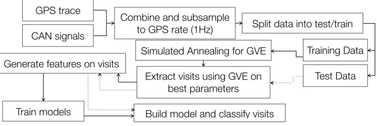
Fig. 1. Overview of experimental methodology

3.2 Labelling

We classify a point of interest with a specific action using the following eight labels (4 positive and 4 negative, as marked).

(1) Drive-through (+): multiple stops and slow movements, at ordering and paying windows. (2) Drop-off (+): the vehicle stops for passengers to exit.

(3) Parked (+): the vehicle is not being driven.

(4) Pick-up (+): the vehicle stops for passengers to enter.

(5) Barrier (-): the vehicle stops for the driver to interact with and proceed past a closed barrier (e.g. a toll booth). (6) Driving (-): normal driving in free flowing traffic.

(7) Manoeuvre (-): several slow movements with the possibility of stationary periods, high direction change and reverse travel (e.g. turn in the road).

(8) Traffic (-): slow movement due to external events (e.g. roundabouts or traffic lights).

We consider four of these labels to be positive (+), i.e. the event is a PoI, and the other four to be negative (-), corresponding to noise in terms of visited locations. With this set of labels, the class distribution is uneven as the traffic labels will be higher in frequency.

Dashcam footage was analysed to determine the activities being performed, in addition to manual logging, to assign ground truth labels to the GPS data. Rules were created for labelling transitions and these were consistently applied throughout1.

4 POI EXTRACTION

To optimise the clustering parameters, we used simulated annealing over a large search space with an appropriate performance metric. The approach to defining a metric was to consider the error in the extracted PoIs when compared to the labels. This metric will be introduced in Section 4.2. The driving and non-driving states were used, denoting the absence and presence of a PoI respectively.

4 J. Van Hinsbergh et al.

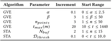
Table 1. Simulated annealing parameter increments

Algorithm Parameter Increment Start Range

GVE α 0.1 0≤α≤2.5

GVE β 3 1≤β≤50

GVE npoi nt s 3 1≤n≤50

GVE tmax(m) 20 10≤t≤1440

STA N_{bu f} 2 1≤n≤15 STA D_{t hr e s h} 0.1 0<t≤10.0

4.1 Methodology

In this paper, we adopt the process shown in Fig. 1. Out of the nine routes, five were used for the training data, with the remaining four used for the test data. Routes were carefully selected to ensure both sets included every label and minimised the use of same roads between testing and training. Due to the temporal nature of the data, separating routes into smaller denominations would create additional false positives for the start and end of each segment.

As in Thomasonet al.[12], we adopt simulated annealing to optimise the parameters for the clustering algorithms, using the increments and start ranges shown in Table 1. In GVE, four parameters affect the extracted PoIs and their properties, as discussed in [13], compared to two parameters in STA [1]. Parameters were initialised within the given range and randomly changed according to the increments shown in Table 1. We ran 1000 instances of simulated annealing, using the same training data in each, but with randomised starting parameters.

After clustering, PoIs are merged using a defined threshold. If the time between the last point in a PoI and the first point in the subsequent PoI is lower than the merge threshold, these PoIs are joined together. In this paper, we considered merge thresholds of 0 and 10 seconds (where 0 seconds prevents any merging).

4.2 Evaluation

When evaluating PoI extraction, two labels were used, namely driving and non-driving. The non-driving label contains all PoIs that are extracted by the clustering algorithm. Different clusters of non-driving are counted as equivalent, and similarly for the driving clusters. The set overlap between the output clusters and the ground truth, namely the Sørensen–Dice coefficient, was used as a performance metric [12], defined as,

QS= 2|A∩B|

|A|+|B|, (1)

whereQSis the quotient of similarity,Ais the set of points in a predicted event andBis the set of points in a ground truth event. Set overlap is limited as it does not consider why parts of the two sets do not overlap, therefore any absence of overlap has equal weighting.

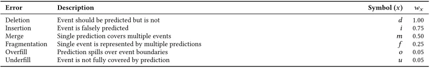
Table 2. Selected error weightings

Error Description Symbol (x) wx

Deletion Event should be predicted but is not d 1.00

Insertion Event is falsely predicted i 0.75

Merge Single prediction covers multiple events m 0.50

Fragmentation Single event is represented by multiple predictions f 0.25

Overfill Prediction spills over event boundaries o 0.05

Underfill Event is not fully covered by prediction u 0.05

To allow comparison between multiple outputs, the error metric must be proportional to the size of the input data. We used the duration, multiplied by the respective error weighting,

W E=

Í

x∈ {d,i,m,f,o,u}wx·sx

st , (2)

whereW Eis the Ward error,xis the error type,wxis the weight given to the error typex,sxis the number of seconds

of error typexandstis the total duration of events (in seconds).

The length for each individual error type will only include the sections that are unmatched for each specific error type. Insertions and deletion errors always span the entire prediction or event. In this approach, the maximum error score is,

wx·sx

st , (3)

whensx=st. This will occur if the total time is a single non-driving event and no predictions were made, implying

the length of the deletion errorsxis equal to the total length of the eventsst. The minimum error is 0, indicating all

predictions and events match.

4.3 Classification of Extracted PoIs

The classification stage aims to filter out false PoIs. This is achieved by using supervised learning with the signals from the vehicle in order to predict the current activity. Once the cluster output is combined with the CAN data, the relevance of PoIs can be assessed. A limitation of this approach is that any PoI erased by the clustering algorithm can not be recovered by the classification stage (that is, a point that was deemed not to be of interest cannot be classified). In this work, we use a SVM [4] alongside minimal redundancy maximal relevancy (mRMR) feature selection [9]. Other classifiers and feature selection methods can be used, but we found this combination to have the highest performance. When training, 10-fold cross validation was used to get a better indicator of model performance.

Given the number of signals and the number of features generated per signal (7 for each real-valued signal, 4 for each categoric signal), there are 90 features available for input into the model. Using mRMR we ranked the topnfeatures and generated models starting with a single feature until all 90 were used.

5 RESULTS

In this section, we present the results of the clustering optimisation using the Ward Metric and set overlap, along with the results for the classification models, designed to determine if the extracted PoI is a true or false positive.

6 J. Van Hinsbergh et al.

Table 3. Classification results, where∗denotes the highest metric used to set the clustering algorithm parameters

Evaluation QS WE # Features Acc. AUC

GVE (0s) 0.512 *0.999 14 0.938 0.948 GVE (10s) *0.598 0.987 34 0.829 0.955 STA (0s) 0.567 *0.664 8 0.935 0.837 STA (10s) *0.593 0.662 21 0.825 0.951

(a) Set overlap (b) Ward Metric

Fig. 2. Averaged simulated annealing performances measured by (a) set overlap and (b) Ward Metric

5.1 PoI Extraction

To evaluate the performance of the parameter sets and clustering algorithms, simulated annealing was conducted using two different merge thresholds of 0 and 10 seconds. We used both set overlap and the Ward Metric, giving 4 different combinations (two methods and two merge thresholds) for both GVE and STA.

Fig. 2a shows the averaged set overlap performance for the four combinations used. The peak performance is achieved when a 10 second merge threshold is used with GVE. A different trend is observed for the Ward Metric (Fig. 2b). The most notable difference is the performance decrease from STA, which is expected as STA does not consider the time between each point and therefore has multiple errors.

Given the differences in performance metrics and clustering algorithms, four parameter sets were chosen, namely the top performing score with each clustering algorithm and evaluation metric combination. This resulted in the parameter combinations shown in Table 3, which were used cluster the training data.

5.2 Activity Classification

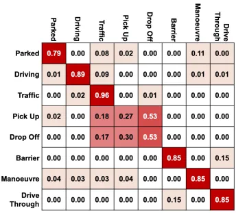
Fig. 3. Confusion matrix for SVM, mRMR with 34 features

With 34 features, the SVM achieves an accuracy of 0.829 with an AUC of 0.95, totalling 119 incorrect classifications. The confusion matrix is shown in Figure 3, which details the accuracies that each label is classified as on the test set. The confusion matrix shows that multiple misclassifications occur between the traffic, pick-up and drop-off classes. This was observed at multiple locations including stations, shopping centres and high streets. If we considered the task as a binary classification problem, the majority of misclassification errors would not be present due to several of the misclassifications being between two positive labels.

Before classification, the clustering algorithm generated 507 false PoIs. These were 20 instances of barriers, 114 driving, 67 manoeuvre and 306 traffic. After the SVM predicted the activity of each cluster, only 15 false PoIs remain, giving an improvement of 33.8 times. Some true PoIs are removed in this process, 34 in total, but this does not outweigh the decrease in false PoIs.

In summary, GVE with a 10 second merge threshold and parameter search guided by set overlap gives the best clustering performance. Moreover, it was found that GVE with a classification model produces the highest performance for point of interest extraction, minimising false positives.

8 J. Van Hinsbergh et al.

6 CONCLUSIONS

In this paper, we investigated two clustering algorithms to extract points of interest on a given journey. We proposed using a classification stage to eliminate false positives within these extracted points of interest. This classification stage uses common signals from the vehicle, such as whether a door is open or not, to predict the context of the proposed point of interest. For the classification, an SVM with features selected using mRMR, eliminated this noise effectively, achieving accuracy of 0.829. This reduces the amount of false positives given by the optimised clustering algorithm by over 33 times.

Being able to robustly extract points of interest for sets of journeys opens up their use in pattern-of-life prediction applications, most notably destination prediction. Doing so allows the input to such an application to be a discrete set of PoIs, rather than a continuous trace of GPS coordinates.

As future work, we aim to analyse further classification approaches, and apply the method to unscripted journeys. This will allow for further analysis between characteristics of activities. We can also investigate the addition of geographical data from sources such as OpenStreetMap, to see if extra information can boost performance.

ACKNOWLEDGEMENTS

This work was supported by Jaguar Land Rover and the UK-EPSRC grant EP/N012380/1 as part of the jointly funded Towards Autonomy: Smart and Connected Control (TASCC) Programme.

REFERENCES

[1] A. Bamis and A. Savvides. 2010. Lightweight Extraction of Frequent Spatio-Temporal Activities from GPS Traces. In31st IEEE Real-Time Systems Symposium. 281–291.

[2] A. Bulling, U. Blanke, and B. Schiele. 2014. A tutorial on human activity recognition using body-worn inertial sensors.Comput. Surveys46, 3 (2014), 33.

[3] M. Ester, H. Kriegel, J. Sander, and X. Xu. 1996. A Density-based Algorithm for Discovering Clusters in Large Spatial Databases with Noise. In

Proceedings of the 2nd International Conference on Knowledge Discovery and Data Mining. 226–231.

[4] E. Frank, M. Hall, and I. Witten. 2016. The WEKA Workbench. Data Mining: Practical Machine Learning Tools and Techniques. (2016). [5] A. Jahangiri and H. A. Rakha. 2015. Applying Machine Learning Techniques to Transportation Mode Recognition Using Mobile Phone Sensor Data.

IEEE Transactions on Intelligent Transportation Systems16, 5 (Oct 2015), 2406–2417.

[6] N. Krishnan and D. Cook. 2014. Activity recognition on streaming sensor data.Pervasive and mobile computing10 (2014), 138–154. [7] L. Liao, D. Fox, and H. Kautz. 2006. Location-based activity recognition. InAdvances in Neural Information Processing Systems. 787–794. [8] A. Palma, V. Bogorny, B. Kuijpers, and L. Alvares. 2008. A Clustering-based Approach for Discovering Interesting Places in Trajectories. In

Proceedings of the ACM Symposium on Applied Computing. 863–868.

[9] H. Peng, F. Long, and C. Ding. 2005. Feature selection based on mutual information criteria of max-dependency, max-relevance, and min-redundancy.

IEEE Transactions on Pattern Analysis and Machine Intelligence27, 8 (2005), 1226–1238.

[10] P. Rashidi, D. Cook, L. Holder, and M. Schmitter-Edgecombe. 2011. Discovering activities to recognize and track in a smart environment.IEEE transactions on knowledge and data engineering23, 4 (2011), 527–539.

[11] S. Reddy, J. Burke, D. Estrin, M. Hansen, and M. Srivastava. 2008. Determining transportation mode on mobile phones. In2008 12th IEEE International Symposium on Wearable Computers. 25–28.

[12] A. Thomason, N. Griffiths, and V. Sanchez. 2015. Parameter Optimisation for Location Extraction and Prediction Applications. InIEEE International Conference on Pervasive Intelligence and Computing. 2173–2180.

[13] A. Thomason, N. Griffiths, and V. Sanchez. 2016. Identifying locations from geospatial trajectories.J. Comput. System Sci.82, 4 (2016), 566 – 581. [14] J. Ward, P. Lukowicz, and H. Gellersen. 2011. Performance Metrics for Activity Recognition.ACM Transactions on Intelligent Systems and Technology