Three essays in international financial economics

(1)

warwick.ac.uk/lib-publications

A Thesis Submitted for the Degree of PhD at the University of Warwick

Permanent WRAP URL:

http://wrap.warwick.ac.uk/130762

Copyright and reuse:

This thesis is made available online and is protected by original copyright.

Please scroll down to view the document itself.

Please refer to the repository record for this item for information to help you to cite it.

Our policy information is available from the repository home page.

(2)

Three Essays in International Financial Economics

by

Kolja Johannsen

Thesis

Submitted to the University of Warwick

for the degree of

Doctor of Philosophy

Warwick Business School

(3)

List of Tables

3.1 Summary statistics of BRL-USD futures market . . . 121

3.2 Spreads . . . 123

3.3 Total arbitrage opportunities . . . 123

3.4 Arbitrage classification . . . 123

3.5 Daily summary statistics . . . 125

3.6 Unbiased information share based on toxic arbitrage (#tox 10) . . . 125

3.7 Comparison of information shares (#tox 10) . . . 126

4.1 Parameters . . . 170

4.2 Four simulation results for parameter setA . . . 171

4.3 Descriptive statistics . . . 171

4.4 Summary of FX exposure . . . 172

4.5 Regression: FX correlation and foreign ownership . . . 173

4.6 Regression: Absolute FX correlation and post-crisis . . . 174

4.7 Regression per country . . . 175

4.8 Regression per country with some foreign ownership . . . 176

4.9 Regression: FX correlation and foreign ownership II . . . 177

(7)

List of Figures

2.1 Bursting bubbles followed bybear market rallies . . . 53

2.2 Cumulative prospect theory (CPT) utility function . . . 54

2.3 Time line . . . 54

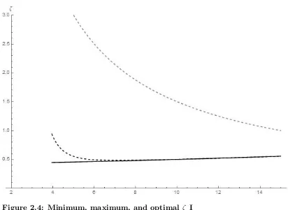
2.4 Minimum, maximum, and optimal ⇣ I . . . 55

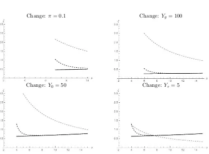
2.5 Minimum, maximum, and optimal ⇣ II . . . 56

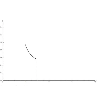
2.6 Proposition 1: Jump in demand . . . 57

2.7 Jump in demand with varying parameters . . . 58

2.8 Anticipated maximum demand . . . 59

2.9 Equilibrium price . . . 59

2.10 Example with dead cat bounce . . . 60

2.11 Example without dead cat bounce . . . 60

2.12 Condition for a dead cat bounce . . . 61

2.13 Jump in demand in Case II . . . 61

3.1 Time line . . . 117

3.2 Choice of informed traderB . . . 117

3.3 Truncated normal distribution . . . 118

3.4 Normal distribution truncated at zero . . . 118

3.5 Model-based simulation . . . 119

(8)

3.7 Model-based simulation: T AIS bounds . . . 120

3.8 Simulation II . . . 120

3.9 Simulation III . . . 121

3.10 Daily traded volume in BMF and CME . . . 122

3.11 Hourly traded volume in BMF and CME in percent . . . 122

3.12 Weekly number of arbitrage opportunities . . . 124

3.13 Price discovery over time . . . 127

3.14 Out of bound observations . . . 127

4.1 Theory results . . . 170

4.2 Simulation results . . . 173

4.3 Coefficient ˆ✓ for per month regression . . . 179

4.4 Coefficient ˆ✓ for per month regression in developed markets . . . 180

(9)

Acknowledgments

“Idle reader, you can believe me when I say that I’d like this book, as a child of my intellect, to be the most beautiful, the most gallant, and most ingenious one that could ever be imagined. But I haven’t been able to violate the laws of nature, which state that each one begets his like.” — Miguel de Cervantes

I cannot think of a better way to describe this thesis which is the product of my PhD than with Cervantes’ words. The image of his ingenious gentleman has for the longest time been part of my home and symbolizes the past years better than any other. As for him, this battling of windmills by abstraction and determination would not have been possible or at least enjoyable without valued companions.

This thesis would not exist without the support and guidance by Michael Moore, who encouraged me to join the program and supervised me for the first three years. Our conversations went far beyond the subject area and I would not be at this point without him. Similarly, I am greatly indebted to Roman Kozhan who did not hesitate to take over as supervisor and provided me with support and advice. Their suggestions and critique have both shaped the past four years and this thesis.

(10)

of frustration. Our late night debates in London, San Francisco, and Leamington Spa are some of my most vivid memories of the past four years. Finally, Miranda Lewis and David Felstead have been anchors of sanity outside the world of research and finance. They helped me keep calm during the ups and downs and this document is also a result of their support.

(11)

Declarations

(12)

Abstract

(13)

Chapter 1

Introduction

This thesis explores di↵erent aspects of international financial markets. The three main chapters, though very distinct in their focus, are aimed at analyzing how international financial markets work. Throughout the thesis, the methodology shifts from a purely theoretical contribution towards a mostly empirical analysis based on theoretical hy-potheses. While Chapter 2 looks at the dynamics of asset prices during financial bub-bles, Chapter 3 focuses on the interaction of di↵erent trading venues both theoretically and, in one example, empirically. In Chapter 4, I provide a new perspective on the link between exchange rates and portfolio diversification by international investors. The purpose of each chapter is to provide new insights into the dynamics and mechanisms which drive international financial markets. The chapters are presented in the form of papers. All three are single-authored.

Chapter 2

(14)

feature in unraveling financial bubbles is the temporary reversal of the downward trend, also known asdead cat bounce orbear market rally. I show that preferences according to cumulative prospect theory can lead an investor to take excessive risk and unprofitable positions in order to recover an initial loss in a declining market. The loss driven be-havior results in premature re-entering into the market. Heterogeneous investors enter at the same time despite di↵erences in their reference points, wealth, and initial loss. The resulting shift in aggregate demand can explain the sudden but temporary reversal common in declining asset prices.

Chapter 3

(15)

Chapter 4

(16)

Chapter 2

(17)

2.1 Motivation

During bear markets, in particular after the burst of a bubble, asset prices often experi-ence a temporary reversal of the downward trend followed by a further decline. Investors commonly describe this phenomenon as dead cat bounce while authors such as Maheu et al. (2012) refer to it as bear market rally. Despite its importance for investors, the

dead cat bounce has widely been ignored by the theoretical literature.

This paper provides a theoretical explanation for the dead cat bounce using in-sights from behavioral finance namely cumulative prospect theory. As a financial bubble bursts investors sell their holdings leading to large perceived losses. In the hope to re-cover these losses, such investors are willing to make excessively risky investments by re-entering the market after a further fall in prices. This re-entering leads to a temporary reversal in the sell-o↵. Thereby, the occurrence of a reversal does not rely on the arrival of fundamental information or coincided closing of short positions which are commonly given explanations.

Temporary reversals in falling prices are a common feature in capital, commodity, and currency markets as shown in Figure 2.1. In March 2000 the NASDAQ composite index saw the peak of a bubble which had been years in the making. Within a bit more than two months the index lost over a third of its value. In the subsequent 8 weeks the index rose by 33% narrowing the gap to its previous high to 15%. After this short lived recovery, the stock index plummeted once again, reaching its low point over two years later ending up with a total loss of nearly 80% compared to its peak.

The need for a better understanding of such events for investors is clearly given. Additionally, central banks and government bodies repeatedly intervene in currency crises and stock market bubbles. The coordinated intervention by China’s “national team” of state financial institutions investing at least $ 140 billion1 in the equity market

1_{This is the estimate in the beginning of August 2015 according to the financial time: ”Goldman}

(18)

to curb the fall in stock prices has been a recent example. A failure to understand the downward dynamics of asset prices can easily lead to a misinterpretation of the success of such measures. If the intervention occurs towards the beginning of adead cat bounce, the upward movement is likely to provide a false sense of success and an early end to supporting measures. The results even indicate that the timing of the temporary reversal may be triggered by intervention.

Similarly, there is a plethora of examples of central bank intervention in the FX market attempting to smooth or even reverse the unraveling of currency bubbles. These attempts are hazardous given the lack in understanding of downward dynamics. The temporary reversal of the downward trend is a natural starting point for a more in depth analysis.

This paper shows that (1) the demand can be split into a loss recovery compo-nent as well as an investment compocompo-nent. The loss recovery compocompo-nent is the amount the investor needs to invest in order to have a chance of recovering his losses. The in-vestment component is what he is willing to invest beyond this point. (2) The demand is “objectively irrational” meaning that the investor will buy the asset despite negative expected return. Further, if he had not su↵ered an initial loss, he would not enter the market at this point. (3) There is a jump in demand from zero to the desired level once the price falls under a threshold, i.e. demand does not follow a continuous function. (4) This jump is likely to coincide among a large group of investors leading to a large and sudden shift in aggregate demand. The resulting jump in overall demand explains the strong, sudden reversal in the downward trend. Furthermore, the reversal can be triggered by trivial events and the end of the reversal does not need new fundamental information.

(19)

maximization problem as well as an analysis of his decision to re-enter. In Section 2.6, I analyze the timing when the investor reconsiders his demand and go into details of the reversal. Section 2.7 provides a brief summary of the results.

2.2 Literature

This paper combines several branches of literature on e.g. bear markets, currency crises, asset pricing, and behavioral finance. Yet, the largest contribution is to the literature on financial bubbles. Kaizoji and Sornette (2008) as well as Scherbina and Schlusche (2014) provide concise reviews of prominent approaches on the latter. From their summaries it becomes clear that the existing literature has focused on the build-up and burst of bubbles, ignoring its unraveling.

The wide interest in financial bubbles is not least found in the cost that bubbles can have for the economy as a whole. Jord`a et al. (2015) analyze these costs, especially in connection with leverage. Similarly, Brunnermeier and Schnabel (2015) provide insights into the history of bubbles by collecting evidence from the main financial bubbles of the last 400 years. The costs also explain the large literature on central bank intervention. Roubini (2006), Posen (2006), and Conlon (2015) are only some examples of a long discussion on whether central banks should burst bubbles. This discussion shows the interest in central bank intervention and the need for a better understanding of its e↵ects. Given the prominence of this question, it is surprising to see no contribution on the dynamics of bursting bubbles.

(20)

Brunnermeier (2008) summarizes the di↵erent approaches by identifying four types of theoretical models for explaining bubbles. These four strands of models are: 1) all investors have rational expectations and identical information, 2) investors are asym-metrically informed and the existence of a bubble need not be common knowledge, 3) rational traders interact with behavioral traders and limits to arbitrage prevent rational investors from limiting the price impact of behavioral traders, 4) investors hold hetero-geneous beliefs and agree to disagree about the fundamental value. This paper can be seen as the aftermath of his third category. In this class of models, limited arbitrage is caused by rational, well-informed and sophisticated investors’ interaction with behavioral traders where the latter are subject to psychological biases. Abreu and Brunnermeier (2003) give an example of such a model. They show why rational arbitrageurs may fail to correct excessive price developments driven by noise traders. Building upon their findings, this paper shows that reversals can happen despite rational arbitrageurs and in absence of fundamental news. Further, I find that the interaction between the inhibited arbitrage in Abreu and Brunnermeier (2003) and the analyzed reversal here is likely to matter for a better understanding of unraveling bubbles.

(21)

matters less in financial research. This is the case as the existing literature focuses on returns close to the reference value. This paper is the first attempt to apply prospect theory to bubbles. In contrast to Barberis (2013), the results in this paper are pri-marily driven by diminishing sensitivity, highlighting its importance in extreme market situations.

Most earlier work in behavioral asset pricing, such as by Barberis et al. (2001), assume loss averse investors to be homogeneous. Berkelaar and Kouwenberg (2009) find that the heterogeneity of investors in wealth and reference point matters. This is to some extent in contrast to the results here that a di↵erence in wealth or reference value has no e↵ect on the re-entering decision but only on the amount demanded.

Apart from the literature on financial bubbles, there is a small literature on bear market rallies. While this is the first theoretical paper on this topic, there has been some empirical work. A central problem in the empirical analysis of bear market rallies is the necessity for a clear definition and a clear separation between bull markets and bear market rallies. Maheu et al. (2012) analyze weekly S&P500 returns between 1885 and 2008 using a four state Markov switching model. The probability of a bear market being turned into a bear market rally is 96%, while the probability for it to turn into a bull market is 4%. This is partly due to the authors definition of a bear market rally which can turn into a bull or bear market. If we define a bear market rally as a period embedded in bear markets, the probability of a bear market to lead to a bear market rally is still 42%.2 _{Maheu et al. (2012) hence emphasize the importance of the phenomenon.} Furthermore, the average cumulative return in the bear market state is -12% while bear market rallies counteract this steep decline by yielding a cumulative return of 7% on average. The authors also conclude that bear market rallies are significantly larger than bull market corrections. Over the 123 years, the S&P500 spent around 16% of the time in

2_{In the authors’ estimation, the probability of a bear market turning into a bull market is 4%, while}

(22)

bear market rallies. These results quantify the importance of understanding downward dynamics and specifically bear market rallies. For future empirical work, my results indicate that it may be worth di↵erentiating between bear market rallies close to the equilibrium level and those closer to the peak.

Overall, theoretical work on downward dynamics such as bear market rallies is scarce. An exception is the literature on fire sales such as by Miller and Stiglitz (2010). The idea that balance sheet e↵ects matter seems to be largely accepted at least in times of crisis. However, fire sales merely exacerbate the downward pressure. It follows, that in presence of fire sales, the mechanism explaining temporary reversals will have to be even stronger. The next section introduces the model set-up and the investor’s preferences.

2.3 Model set-up

This model focuses on an investor’s portfolio reevaluation during the unraveling of a bubble after su↵ering an initial loss.

Consider an investor with preferences according to cumulative prospect theory (CPT) as introduced by Kahneman and Tversky (1979). The investor’s utility function is split into a concave part for gains with respect to a reference value and a convex part for losses. This implies risk seeking behavior once losses have occurred and risk averse behavior after gains. Figure 2.2 illustrates the CPT utility function.

Using experimental data, Tversky and Kahneman (1992) find that the utility function is best described as

u(x) =

8 > < > :

u+(x) if x 0 u ( x) if x <0

(2.1)

(23)

In line with the experimental evidence by Tversky and Kahneman (1992), I as-sume 0.5<↵= <1. It is worth mentioning that while Bernard and Ghossoub (2010) depend on↵< for an interior solution in a model similar to this one, this assumption is not necessary here. Tversky and Kahneman (1992) find a loss aversion parameter of ⇡2.25. A higher loss aversion parameter leads to a stronger punishment for losses. For simplicity and without change in the results,3 let be set to unity.

Assumption 1 The investor’s utility function is given by

u(x) =

8 > < > :

x if x 0 ( x) if x <0.

with0.5< <1.

Following Kahneman and Tversky, x is given by the change of wealth relative to a reference value Y0. In this model, I refrain from a fix definition of the reference value. Generally, it can be thought of as the expectation or aspiration the investor has for the asset. Given that the focus here is on financial bubbles, the reference value is likely to be inflated and overly optimistic. The change in wealth is dependent on the investor’s demand for a single risky asset. Without loss of generality, assume that the risk-less alternative yields zero interest. The risky asset has two possible outcomes. With probability⇡ the asset yields a high final valueYg and with probability (1 ⇡) the asset realizes a final value Yb < Yg. Given a bubble setting, the good state can be considered less likely:

Assumption 2 The probability of the positive outcome is given by

⇡<0.5.

(24)

Due to their nature, bubble assets are likely to be perceived as having quasi binary outcomes. As an example, consider Internet stocks in the late 1990s. Investors hoped to “find the next Amazon” leading to large gains. At the same time, there was a large risk of bankruptcy for firms which did not become profitable. This makes the assumption of binary outcomes more sensible than in other settings.

In line with Kahneman and Tversky (1979), the probability ⇡ is subjective. Agents perceive probabilities in a distorted way where low probabilities are seen as larger, while larger probabilities are undervalued. In this setting, there is no need to specify what the objective probabilities are.

Figure 2.3 illustrates the chronological setting of the model. While the bubble grows, the investor enters the market buying one unit of the asset. For simplicity, assume that this is all his disposable wealth.4

Assumption 3 The investor invests all his disposable wealth into the risky asset when first entering.

The investor now forms his reference value Y0. In contrast to the existing literature, I refrain from imposing a functional form on the reference value.5 One can think of Y0 as the price that the investor is convinced the asset will reach.

The burst of the bubble is assumed to be caused by a change in market expecta-tion, leading to the subjective expected value

E(vs) :=⇡Yg+ (1 ⇡)Yb. (2.2)

After the bubble bursts, the investor sells all his assets to price Yr < Y0.

Conse-4_{Assumption 3 is not a necessary assumption for the results in this paper to hold. Section 2.8.11}

provides more details on the e↵ect of retained wealth. Overall, the behavior of the investor does not change, however additional savings relax the budget constraint and make the condition to observe loss driven behavior more restrictive.

5_{Most authors like Barberis et al. (2001), Gomes (2005), and Bernard and Ghossoub (2009) use the}

(25)

quently, he realizes a loss with respect to his reference value of (Y0 Yr). By assumption, the CPT investor is not able to engage in short selling. This is a reasonable assumption when seeing the CPT investor as less sophisticated.

Assumption 4 No short selling by the CPT investor.

From this point onward, the CPT investor is loss-driven. He is willing to take large risks hoping to recover his losses. After a further fall in the price top, the investor decides on his new portfolio ⇣. The timing of the decision is hence exogenous6 while the amount invested is endogenous. A larger ⇣ implies a larger exposure to the risky asset. Due to the short selling constraint, ⇣ 0 must hold. Further, given that the investor sold his holdings at price Yr the investor faces a budget constraint7 of ⇣p Yr. Hence, the bounds of the new portfolio holdings are given by

0_⇣ _ Yr

p . (2.3)

p < Yrimplies that the upper bound is larger or equal to one and increasing with a lower price p. As the price falls further, an investor is able to buy a larger amount of the asset. Finally, the investor realizes eitherYg or Yb. Without loss of generality, I set Yb >0. This allows us to interpret Yg, Y0, Yb, Yr,and p as price levels.

Assumption 5 The hierarchy of price levels as explained above is summarized as

Yg > p > Yb and Y0 > Yr> p.

6_{In this model, the timing when the investor reconsiders his portfolio is exogenous. This is a strong}

simplification as it implies the absence of intertemporal optimization. However, the setting is sufficient to show how the willingness of the investor depends on the price of the asset and to demonstrate the discontinuous reaction in demand resulting from CPT preferences.

7_{This budget constraint results from Assumption 3 that the investor is fully invested at the height}

(26)

This paper can be limited to cases where the investment yields a negative sub-jective expected value. The limitation is justified as I am considering reversals at the height of the unraveling. If the asset yielded a positive return, the investment would be attractive for risk neutral investors as well. In this case, there would be no further downward pressure in the price and the reversal would not be temporary. Put di↵erently, without selling pressure the asset would be close to its equilibrium price. This implies that the reconsideration would occur towards the end of the unrevealing rather than at its height.

Assumption 6 The risky asset has a negative expected return

⇡(Yg p) (1 ⇡)(p Yb)<0.

Assumption 6 provides a lower bound for the price when considering to re-enter, given by:

p >⇡Yg+ (1 ⇡)Yb. (2.4)

Given Assumptions 1 and 2 that <1 and ⇡ <0.5, Assumption 6 also implies that an investor with CPT preferences who has not su↵ered an initial loss would not invest into the risky asset, as

⇡(Yg p) (1 ⇡)(p Yb) <0. (2.5)

(27)

2.4 The investor’s maximization

This section focuses on the investor’s maximization problem when choosing the optimal portfolio⇣. There are two cases which need to be considered.

I) The investor is able to recover his initial losses with respect to his reference value in the good state.

II) Even with the good outcome, the investor cannot recover his initial loss with respect to his reference value.

In the latter case, this implies that the whole maximization takes place in the convex part of the utility function. It is crucial to keep in mind that the utility in the good state depends on the endogenous variable ⇣. This implies that it depends on the size of ⇣ whether the agent can recover his losses and hence which case needs to be considered.

2.4.1 Case I: Complete recovery of losses possible

For now, let us assume that the investor makes an overall gain if the outcome is positive, i.e. Case I. It follows that given the utility function in Assumption 1, the investor’s subjective expected utility when creating his optimal portfolio is given by

E(U) =⇡u+(xg) + (1 ⇡)u (xb)

=⇡(xg) (1 ⇡) ( xb) . (2.6)

Following the setting above, xg and xb are given by initial loss Y0 Yr and the gain and loss from the reinvestment, respectively:

(28)

It follows that

E(U) =⇡[⇣(Yg p) (Y0 Yr)] (1 ⇡)[ (⇣(Yb p) (Y0 Yr))]

=⇡[⇣(Yg p) (Y0 Yr)] (1 ⇡)[⇣(p Yb) + (Y0 Yr)] . (2.7)

Loss recovery in the good state implies therefore that⇣(Yg p) (Y0 Yr) 0. For Case I to be true, the optimal investment needs to be at least

⇣M in =

Y0 Yr Yg p

. (2.8)

The minimum investment is needed to have a chance to recover the initial loss. It represents the ratio of the initial loss with respect to the reference value and the potential gain by investing into the risky asset. Together with the upper bound, the minimum ⇣ for Case I leads to

Y0 Yr Yg p 

⇣_ Yr p

p_Yg Yr Y0

. (2.9)

This is the condition for Case I, i.e. for total loss recovery to be possible. It is important to note that this is independent of the bad outcome. Hence, the case di↵erentiation is not connected to the expected value but only to the size of the positive outcome.

The investor’s maximization problem is given by

max

⇣ E(U), (2.10)

leading to the following proposition:

(29)

investor invests a positive amount given by ⇣⇤ up to his budget constraint, where

⇣⇤ = (Y0 Yr) (p Yb)

1 +⌦

⌦ ⌦ (2.11)

with⌦= Yg p

p Yb >0, =

⇡

1 ⇡ >0 and = 11 >2. He does so despite negative expected

returns.

Proof. See Appendix 2.8.1.

⌦is the ratio of the outcome in the good state and the absolute of the outcome in the bad state. ⌦>1 implies that the gains in the good state exceed the losses in the bad state. is given by the ratio of the subjective probability for the good state and the subjective probability of the bad state. <1 implies that the good state is perceived as less likely. Given that ⇡ <0.5, I find <1. Following the definitions above,⌦ is the probability weighted outcome ratio. A ⌦ < 1 implies a negative subjective expected value, which is equivalent to Assumption 6.

provides the elasticity of intertemporal substitution. A larger implies a higher elasticity of intertemporal substitution and, hence, lower cost for a suboptimal distribution of consumption across periods. In this setting, this is equivalent to lower cost for an uneven distribution across the states of nature.

Lemma 1 shows the importance of loss recovery. When incentivized by even a remote chance to recover losses, the investor will invest a positive amount even if he expects negative returns.

Corollary 1 The optimal investment can be decomposed into a loss recovery component

⇣M in and an investment component IC:

(30)

where

⇣M in =

Y0 Yr Yg p

>0 and IC = ⌦

2 _{(1 +}_⌦₎₍_Y 0 Yr) (1 ⌦ 1 ₎₍_p _Y

b)

>0. (2.13)

The recovery component is the amount necessary in order for the investor to have a chance to recover his initial losses. The investment component is given by the remainder.

The loss recovery component ⇣M in results from risk seeking behavior i.e. the convex part of the utility function. The investment component, in contrast, results from the concave part which corresponds to risk aversion.

As mentioned before, the optimization problem is only correctly specified if the optimal⇣⇤ in Equation (2.11) fulfills the minimum⇣ condition in Equation (2.8). Equa-tion (2.12) shows that this condiEqua-tion is fulfilled for all ⇣⇤ as IC > 0. Let us now take a closer look on the e↵ect of price p. Given that I am analyzing the unraveling of a bubble, it makes sense to look at what happens when the price falls further. It can be shown that:

Corollary 2 A lower price leads to a larger investment component and a lower loss recovery component of ⇣⇤.

(31)

recovery component dominates for high prices as the investment remains unprofitable. However, for sufficiently low prices, the investment component takes over and rapidly increases with falling prices driving the overall demand up.

Figure 2.5 illustrates the e↵ect of a change in the parameter values of ⇡, Yg, Y0,and Yr, respectively. In the upper two cases, an increase in⇡ and Yg, respectively, leads the risky asset to be more lucrative. Hence, for this specification the investment component drives the demand even for higher values of p. In the bottom left case, an increase in the reference value leads to an upward shift of both minimum and optimal demand. This is the case as the investor is loss driven and a larger loss leads to a higher willingness to invest. Similarly, a larger loss due to a lowerYrshifts both minimum and optimal demand up. Additionally, the budget constraint is more restricting due to the lower recovery.

2.4.2 Case II: Only partial recovery of losses possible

Now consider the case, where it is impossible for the investor to recover his losses fully. The expected utility function is consequently given by

E(U) =⇡u (xg) + (1 ⇡)u (xb)

= ⇡[ ⇣(Yg p) + (Y0 Yr)] (1 ⇡)[⇣(p Yb) + (Y0 Yr)] . (2.14)

The investor’s optimization in Case II leads to the following lemma:

Lemma 2 Given Assumptions 1, 2, 3, 4, 5, and 6: Whenever the investor has no chance to regain his losses he either invests all he can or nothing.

(32)

will not invest anything. This is e.g. the case when the investment implies a certain loss. If the terms are acceptable, the investor will invest all his disposable wealth into the asset in order to have a chance to get as close as possible to recovering his prior losses. He perceives the riskiness of the asset positively, as an increase in the spread of good and bad states gets him,ceteris paribus, closer to recovering his losses.

Combining the two cases and by that Lemmas 1 and 2 leads to the following: If the investor chooses to re-enter the market, he will invest⇣⇤up to his budget constraint.

⇣⇤ = 8 > < > :

(Y0 Yr)

(p Yb)

1+⌦

⌦ ⌦ if

(Y0 Yr)

(p Yb)

1+⌦

⌦ ⌦  Ypr Yr

p if

(Y0 Yr)

(p Yb)

1+⌦ ⌦ ⌦ >

Yr

p.

(2.15)

In a final step, it is necessary to evaluate when the investor will re-enter, i.e. when the utility from investing is larger than the utility from abstaining from the market.

2.5 The decision to re-enter

The focus of the analysis is the investor’s willingness to re-enter the market given that he reconsiders his absence from the market at a specific point in time. In order to determine this, I compare the investor’s utility from remaining outside the market and re-entering.8 An investor compares re-entering and investing ⇣⇤ to the certain loss when ab-staining the market. For re-entering to be optimal, the following condition needs to be fulfilled

E(U(⇣⇤)) E(U(⇣ = 0)).

Lemma 3 Given Assumptions 1 and 6: The condition for re-entering and hence for

8_{In the following sections, I am focusing on interior solutions for the optimal investment, i.e. cases}

(33)

positive demand is given by

⇡

✓

IC ⇣M in

◆ ✓

1

⌦

◆

1 1_0. (2.16)

Lemma 3 describes the moment when an investor is willing to re-enter the market. Any investor, for whom this condition is not fulfilled, will not re-enter the market upon reconsidering his portfolio. It is important to keep in mind that this model focuses on a bear market. Consequently, this paper aims at answering the question what happens when the price falls and whether this leads to a sudden increase in demand. Lemma 1 and Lemma 3 lead to the following conclusion:

Proposition 1 When p falls, the “potential” demand, i.e. the desired amount invested upon reconsideration, jumps from zero to the optimal level.

The implication here is that this sudden jump can be responsible for the tempo-rary reversal of the downward trend. The size of the jump in demand is given by the optimal demand in Equation (2.11) as the investor has no holding prior to re-entering.

⇣⇤ = (Y0 Yr) (p Yb)

1 +⌦

⌦ ⌦

(34)

the other, he is willing to invest large amounts into an asset which he sold o↵previously. At this point, the expected return of the asset is still negative.

The four graphs in Figure 2.7 highlight the ceteris paribus e↵ect of an increase in the probability of the good state ⇡, a better outcome in the good stateYg, a higher reference value Y0, and a decrease in the recovery price Yr, respectively, compared to Figure 2.6. Doubling the probability⇡ leads to a similar size in the jump, yet the jump occurs earlier, i.e. for higherp. This is intuitive as a higher⇡ implies a more profitable investment. The same is true for an increase in the good outcome. In the latter case, however, the investment reaches only around 34% of the prior holdings.

The two bottom graphs show an increase in the reference value and a decrease in the recovery rate, respectively. Both are equivalent to a higher loss with respect to the reference value and hence have the same e↵ect. The only di↵erence is that a change inYr lowers the budget constraint, restricting the slope of the demand for lowp. The reaction to a change in the initial loss leads to the main result of the paper. Using Lemmas 1 and 3 it follows that:

Proposition 2 The decision to re-enter is independent of the initial loss; however, the size of the potential investment positively depends on it.

A group of investors with similar expectations about the asset’s true value are willing to re-enter the market at a similar time, independently of their prior losses and reference value. However, the size of each investor’s investment will di↵er. The above implies that the timing of the reinvestment is also independent of the disposable wealth.9 The results agree with Berkelaar and Kouwenberg (2009) on that the hetero-geneity of investors with regard to wealth and reference value matters. In this setting, however, the implications are quite di↵erent. While the heterogeneity is important to

9_{This is true, as long as the disposable wealth is su}_ffi_{cient to allow for the optimal investment. If this}

(35)

explain the size of individual demand, the timing is not a↵ected. This implies that from a macro perspective, the heterogeneity matters much less as the individual demand jumps at the same time leading to a jump in aggregate demand. Given the importance of the timing in this setting, the next section goes into it in more detail.

2.6 Equilibrium price

The above analysis has so far considered the CPT investor in isolation. This section takes the previous results further by looking at the interaction of multiple CPT and risk-averse (RA) investors. The model proposed here is not a standard general equilibrium model, but describes how the market reaches its equilibrium.

The layout of the model is summarized as follows. In period 0, the CPT investors update their rational expectations about the pay-o↵s of the asset and trade with the RA investors before the latter update their own expectations. The RA investors do not know the exact demand function of the CPT investors. Therefore, in period 1 the RA investors submit sell orders anticipating the maximum possible demand of the CPT investors to a given price. The anticipated maximum demand, however, assumes the demand function of the CPT investors to be continuous.10 _{This creates a disparity between the anticipated} demand and the actual demand due to the jump in the latter. Consequently, there are two possible cases. If the actual demand falls short of the anticipated maximum demand, the RA investors submit further sell orders in the next periods until the market is in equilibrium.11 If the actual demand exceeds the anticipated demand, this implies that the orders submitted by the RA investors imply too low a price. It follows that the price will rise in the following period in order to bring the market into equilibrium. This reversal in the price is what is described as a dead cat bounce. This set-up is formalized

10_{One option is that the RA investors simply ignore the influence of the perceived loss by the CPT}

investors. I keep the function general in order not to pose strong restrictions.

(36)

below.

Assumption 7 The total amount of investors and assets is normalized to unity. n

investors are risk-averse (RA), while1 nare CPT investors, following the optimization behavior described above. At the start of the bear market, a total amount x of the asset is held by RA investors and (1 x) is held by CPT investors.

The number and holdings of RA versus CPT investors allows to di↵erentiate between di↵erent asset classes. While traditional currency or commodity markets may be dominated by sophisticated RA investors, cryptocurrencies may be thought of as CPT dominated. This idea is in line with Bianchi and Dickerson (2018) who argue that cryptocurrency markets see higher trading volume by retail investors while the number of institutional investors and hedge funds is lower than in other markets. For brevity, I normalize the updated pay-o↵of the asset to

Assumption 8 The pay-o↵ of the asset in the good state is normalized to 1, while the bad state’s pay-o↵ is set to 0 such that

Yg = 1 and Yb= 0. (2.17)

Assumption 9 Assume that all CPT investors receive information that the asset is overvalued before the RA investors do. The CPT investors are hence able to sell all their holdings to price p0 to the RA investors, where p0 is determined by the RA investors

expectations before receiving the update.

The results do not necessarily depend on the strict form of this assumption. Similar to the assumption that the CPT investor liquidates all holdings at priceYr, this assumption simplifies the model in order to focus on the motivation of the CPT investor. A more gradual sell-o↵ is also possible and would likely lead to very similar results.12

(37)

After learning about the updated pay-o↵structure of the asset, the RA investors’ demand for the asset is determined by the maximization of their utility function.

Assumption 10 Each RA investor maximizes a CRRA utility function given by

URA=⇡(Xg)↵+ (1 ⇡)(Xb)↵, (2.18)

where 1 ↵ is the degree of risk aversion of the RA investor, Xg is the wealth in the

good state, and Xb is the wealth in the bad state.

In contrast to the CPT, the CRRA utility function is taking into account the total wealth, rather than the change in wealth.

Assumption 11 The total wealth of the RA investor in the good state is given by

Xg = x

nYg+ (Yg p) +W + (Y g p0) 1 x

n

= x

n+ (1 p) +W + (1 p0) 1 x

n

= 1

n+ (1 p) +W p0 1 x

n . (2.19)

In the bad state, this is equivalent to

Xb = x

nYb+ (Yb p) +W + (Yb p0) 1 x

n

= p+W p01 x

n . (2.20)

(38)

the asset held by RA investorsx, divided by the number of RA investorsn. The amount purchased by an individual RA investor is given by . p corresponds to the price he is paying. W is given by the exogenous, independent wealth of the RA investor and (Y g p0)1_nx is the profit from buying all of the CPTs’ asset holdings. In the bad state, the total wealth is derived equivalently.

The maximization of the RA investors’ utility results in an optimal change in demand ⇤. For this analysis, it makes sense to consider the total supply.

Lemma 4 The total supply is given by the total amount of assets to be sold by the n

RA investors

S(p) = n ⇤= n(W p0

1 x

n )(⌦✏ ✏ 1) n1 p(⌦+⌦✏ ✏₎

= 1 (W n p0(1 x))(⌦

✏ ✏ ₁₎

p(⌦+⌦✏ ✏₎ , (2.21)

where ✏= ₍₁1_↵₎ is one over the risk aversion parameter. The supply function S(p) is a concave function increasing in price p.

(39)

from supplying less. The RA investors, therefore supply in order to meet the maximum demand they deem possible. Thereby, the RA investors are more careful than in standard equilibrium models.13

Assumption 12 Given a price pt in the current period and a price pt+1 in the next

period, the anticipated maximum demand is given by ⌥pt(pt+1), with ⌥pt(pt) = 0,

@⌥_pt(pt+1)

@pt+1 <0 and

@2_⌥

pt(pt+1)

@pt+1@pt+1 >0. Once the suppliers observe a positive demand, they

can anticipate the actual demand.

The definition of⌥pt(pt+1) is kept fairly independent on purpose in order to keep

the results general but interpretable. If the actual demand is equal to the anticipated maximum demand, the market will be in equilibrium. This is the standard case consid-ered in general equilibrium models. If the demand remains non-positive, the suppliers will repeat the step above, using the anticipated maximum demand function⌥pt+1(pt+2).

If the demand is positive but below the supply, it is optimal for the suppliers to lower the price further. They will lower it more cautiously however taking into account the current level of demand.

Figure 2.8 illustrates the procedure described above. The x-axis shows the price and a move from right to left implies a devaluation. As the price falls, the anticipated maximum demand is increasing until it reaches the supply function at pricep1. This is the maximum price, which the suppliers expect to lead to an equilibrium. They hence choose to supply the amountS(p1) in this period. As there is no demand, the suppliers use the anticipated maximum demand function once more in the next period, leading to the supply ofS(p2).

This describes the development of the supply by the RA investors. In the next step, let us consider the equilibrium in the market given by the (actual) aggregated

13_{In order to not make it optimal to submit sell orders for the whole supply, we could assume that there}

(40)

demand and the total supply. The total demand of the CPT investors given Assumptions 7, 8, and 9 is given by

D(p) = (1 n)⇣⇤(p) = (1 n)

✓

1 x 1 n

◆ ✓

Y0 p0

p

◆

(1 +⌦ ) (⌦ ⌦ ) = (1 x)

✓

Y0 p0

p

◆

(1 +⌦ )

(⌦ ⌦ ). (2.22)

The efficient pricep⇤ is hence given by D(p⇤) =S(p⇤). Figure 2.9 illustrates the equilibrium. Let us denote the price at the re-entry of the CPT investors by pR. As highlighted in Proposition 2, this point is independent of the initial loss and will hence be the same for heterogeneous investors.

The next part combines the anticipated maximum demand and the actual demand function. Figure 2.10 illustrates an example where the model exhibits adead cat bounce. At the first intersection of the anticipated maximum demand and the supply function, at pricep1, the actual demand is zero. At the second intersection atp2, the actual demand exceeds the anticipated demand, due to the jump atpR. It follows that in period 1, there is no trade and the price is set to p1. In period 2, the price falls to pricep2 and ⌥p1(p2)

units are traded. As demand exceeds supply at this point, the price will increase over the next periods until it reaches the equilibrium level p⇤. Consequently, after falling to p2, the price experiences a reversal rising by p⇤ p2. This is the size of the dead cat

bounce.

Similarly, Figure 2.11 shows an example, which does not lead to a reversal. In period 1, the price reachesp1. The actual demand given by the black line is not equal to the supply, however, it is positive. Consequently, D(p1) of the asset is traded. Having now observed the actual demand, the suppliers will supply only as much in the next period as is necessary to meet the actual demand at pricep⇤. There is no overshooting in the price and no reversal.

(41)

there is a dead cat bounce, depends on the relative size of the equilibrium price p⇤, the re-entry pricepR, the point where the supply function is zeroS 1(0) and the intersection of the anticipated maximum demand with the supply function (pt). This is illustrated in figure 2.12.

Lemma 5 There exists a dead cat bounce, i↵ the intersection of the anticipated maxi-mum demand with the supply function falls between the price for zero demand and the equilibrium price:

S 1(0)< pt< p⇤ (2.23)

In contrast, there is no dead cat bounce, if the intersection of the anticipated maximum demand with the supply function falls between the equilibrium price and the re-entry price:

p⇤ _ptpR (2.24)

The size of the dead cat bounce is determined by the distance between the equilibrium price and the intersection: p⇤ pt.

The first implication to be drawn from this is that the size of thedead cat bounce

cannot exceedp⇤ S 1(0). Apart from this, the results are very sensitive to the starting value when the RA investors begin to anticipate the CPT investors’ demand as well as the functional form of the anticipated demand. For this reason, it is more meaningful to state the results in terms of probabilities and expectations dependent on the starting value. The model extension in this section leads to a series of testable predictions.

Proposition 3 Given the interaction of multiple CPT and RA investors:

(42)

(b) The larger the share of RA investorsn, the smaller is the possible dead cat bounce. (c) A lower share of RA investors n or a lower share of initial holdings held by RA investors xcan increase the probability that the dead cat bounce happens in a later period.

Proposition 3a) states, a higher reference value of the CPT investors, e.g. due to more optimism at the build up of the bubble, increases the probability of a dead cat bounce as well as its expected size. This is due to the same e↵ect observed in Proposition 2. A higher reference value leads to a higher perceived loss and thereby to a larger demand upon re-entering. The larger jump in demand means, that the di↵erence between the anticipated maximum demand and the actual demand is larger. This leads to a larger reversal and also increases its probability.

According to Proposition 3b), a larger share of RA investors reduces the size of a possible dead cat bounce. The reason for this is that the amount of the asset held by each RA investor x_n is smaller compared to his wealthw. Due to this, the RA investors are overall willing to take more risk. This increases the supply for the asset by RA investors when the asset has negative expected returns in which case the RA investors engage in short selling. This makes the aggregate supply more price sensitive in this area. Consequently, the di↵erence between the prices for which the supply meets the anticipated maximum demand and the actual demand shrinks and the possibledead cat bounce shrinks as well.

(43)

a later period increases. If the RA investors held a lower share before the beginning of the bear market (a lowerx), this decreases each RA investors total wealth equally in the good and in the bad state as can be seen in Assumption 11. Due to their risk aversion, this implies that a lower initial share x leads to a larger punishment for the di↵erence in outcomes. This decreases the amount a RA investor is willing to sell in excess of his holdings (short selling). This in turn increases the price for which the supply curve and the anticipated maximum demand intersect. As above, this is equivalent to saying the probability that there is adead cat bounce in a later period increases conditional on there being a dead cat bounce at all.

2.7 Conclusion

Unraveling bubbles in capital, currency, and commodity markets often experience tem-porary reversals of the downward trend, also known as dead cat bounce or bear market rally. This is the first paper to o↵er a theoretical explanation for a phenomenon which is largely recognized in financial markets.

(44)

impact on the price. Due to the discontinuous demand functions, a minor adjustment in the expected return can lead a group of investors to re-enter the market at the same time. Thereby, seemingly unimportant information can trigger a bear market rally even under heterogeneous expectations.

The model proposed here leads to several testable results. A lower share of unsophisticated investors (CPT investors) is associated with a smallerdead cat bounce. A higher share of unsophisticated investors or a higher share of holdings by unsophisticated investors during the peak of the bubble increase the probability that a price reversal happens at a later point in time, i.e. that there is a longer period between the peak of the bubble and thedead cat bounce. Finally, the larger the optimism during the build-up of the bubble, the higher the probability of adead cat bounce and the larger its expected size.

This paper provides a new mechanism explaining the temporary reversal of the downward trend in unraveling bubbles. There are several other papers that have shown mechanisms which are likely to interact with the one above. Some, such as fire sales described by Miller and Stiglitz (2010) work against the reversal and hence highlight the size of the demand necessary to match the downward pressure. Others, such as herd behavior and limited arbitrage are likely to support the reversal once it started. Kaizoji and Sornette (2008) and Kaizoji (2010a,b) analyze the e↵ect of herd behavior in financial markets. On the one hand, herding puts additional pressure on the price once it starts falling, on the other hand, it is also likely to amplify the reversal. Abreu and Brunnermeier (2003) show that arbitrageurs may forgo betting against a bubble when uncertain about the timing of the burst. This bubble riding behavior is likely to appear during the reversal as well, prolonging its existence further.

(45)

mechanism shown in this paper interacts with the intertemporal optimization as well as investors herding and fire sales. A further analysis in a multi-asset setting is also likely to provide valuable insights. Additionally, it is crucial that we gain better insights into the empirical side of the reversal,dead cat bounce, orbear market rally in the aftermath of financial bubbles. The existing research on bear market rallies is limited to the stock market. The commonness of the phenomenon in FX as well as commodity markets raises the question to what extent the reversals di↵er from one another. Further, the analysis indicates that reversals may di↵er depending on whether they occur in the middle of the fall in prices or mark the end of the unraveling.

(46)

2.8 Appendix

2.8.1 Proof of Lemma 1

The maximization problem in Case I is given by

max

⇣ E(U), (2.25)

which leads to the first order condition

@E(U)

@⇣ =⇡ [⇣(Yg p) (Y0 Yr)] 1₍_Y

g p)

(1 ⇡) [⇣(p Yb) + (Y0 Yr)] 1(p Yb) = 0 (2.26)

) ⌦ [⇣(Yg p) (Y0 Yr)] 1 = [⇣(p Yb) + (Y0 Yr)] 1

⌦ [⇣(p Yb) + (Y0 Yr)]1 = [⇣(Yg p) (Y0 Yr)]1

⌦ [⇣(p Yb) + (Y0 Yr)] = [⇣(Yg p) (Y0 Yr)] ⇣((Yg p) (p Yb)⌦ ) = (Y0 Yr)(1 +⌦ )

⇣⇤ = (Y0 Yr) (p Yb)

1 +⌦

⌦ ⌦

with⌦= Yg p

p Yb >0, =

⇡

1 ⇡ >0 and = 11 >2. The second order condition is given by

@2_E₍_U₎

@⇣@⇣ =⇡ ( 1)[⇣(Yg p) (Y0 Yr)] 2₍_Y

g p)2

(47)

) ⌦22 21 _[⇣(_p _Y

b) + (Y0 Yr)]>[⇣(Yg p) (Y0 Yr)] ⇣(⌦ ⌦22

1

2 ₎₍_p _Y

b)<(Y0 Yr)(1 +⌦

2 2

1

2 ₎_.

Using⇣⇤ from the first order condition leads to

Y0 Yr p Yb

1 +⌦

⌦ ⌦ (⌦ ⌦

2 2

1

2 ₎₍_p _Y

b)<(Y0 Yr)(1 +⌦

2 2

1

2 ₎

1 +⌦

⌦ ⌦ (⌦ ⌦

2 2

1

2 ₎_<_{(1 +}_⌦

2 2

1

2 ₎

⌦22 1

2 ₊_⌦ +1 _<_⌦(1+

2

2 )

1

2 _⌦

⌦ <⌦.

It is straightforward to show, that this second order condition is equivalent to Inequality (2.5) which follows from Assumption 6:

⌦ <⌦

⌦ <1 ⇡

1 ⇡

✓

Yg p p Yb

◆

<1

⇡(Yg p) (1 ⇡)(p Yb) <0.

It follows that ⇣⇤ is the optimal demand under Case I.

Finally, let us consider the upper bound. Given the single extreme value shown by the first order condition, the optimal value must be given by the upper bound, whenever ⇣⇤ exceeds the upper bound given by the budget constraint Yr

p.

(48)

2.8.2 Proof of Corollary 1

Corollary 1 follows from a simple transformation of Equation (2.11):

⇣⇤ = (Y0 Yr) (p Yb)

1 +⌦

⌦ ⌦

= (Y0 Yr) (Yg p)

⌦1 +⌦

⌦ ⌦

= (Y0 Yr) (Yg p)

1 +⌦ ⌦ 1 +⌦ 1

1 ⌦ 1 = (Y0 Yr)

(Yg p)

✓

1 +⌦

1 _{(1 +}_⌦₎ 1 ⌦ 1

◆

= (Y0 Yr) (Yg p)

+(Y0 Yr) (Yg p)

⌦ 1 _{(1 +}_⌦₎ 1 ⌦ 1 =⇣M in+

(Yg p)⌦ 2 (1 +⌦)(Y0 Yr) (p Yb)(1 ⌦ 1 )(Yg p) =⇣M in+

⌦ 2 (1 +⌦)(Y0 Yr) (1 ⌦ 1 ₎₍_p _Y

b) =⇣M in+IC.

Further, given Inequality (2.5), it can be shown that

⇡(Yg p) (1 ⇡)(p Yb) <0

⌦ <1

⌦ 1 <1.

This implies thatIC >0 must hold. ⌅

2.8.3 Proof of Corollary 2

The loss recovery component⇣M in = (Y0 Yr)

(Yg p) is given by Equation (2.8). It follows

(49)

Hence, as the pricep falls, the loss recovery component declines as well. From the proof in Appendix 2.8.2 it is clear that IC can be written as

IC = (Y0 Yr) (Yg p)

⌦ 1 (1 +⌦)

1 ⌦ 1 .

For simplicity, let us denote

= ⌦

1 _{(1 +}_⌦₎

1 ⌦ 1 .

It follows thatIC =⇣M in . This allows us to analyze the components separately

@ @p =

@⌦

@p

⌦ 1+ ( 1)⌦ 2 1 ⌦ 1 + ⌦ +⌦ 1 ( 1)⌦ 2

(1 ⌦ 1 ₎2

!

= @⌦

@p (1 ⌦ 1 ₎2 ( 1)⌦

2₊_⌦ 1 _⌦ 1

= @⌦ @p

⌦ 2

(1 ⌦ 1 ₎2( 1 + ⌦ ⌦ ). (2.27)

As @_@p⌦ = @

Yg p p Yb

@p <0, >2, and Inequality (2.5) holds, it follows that

@

@p >0. (2.28)

Hence, a fall in the price leads to an increase in . As @⇣M in

(50)

two contrary forces within the investment component. It can be shown that

@IC @p =

@⇣M in

@p ⇣M in @

@p (2.29)

= Y0 Yr (Yg p)2

2( 1)⌦ ( 2)⌦ 1 _⌦2 2 _⌦ +1 _⌦ 1 (1 ⌦ 1 ₎2

(2.30)

>0. (2.31)

A lower price leads to a larger investment as the e↵ect on dominates the e↵ect on ⇣M in. ⌅

The first order condition for the investor’s maximization problem in Case II is given by

@E(U)

@⇣ =⇡ [ ⇣(Yg p) + (Y0 Yr)] 1₍_Y

g p)

(1 ⇡) [⇣(p Yb) + (Y0 Yr)] 1(p Yb) = 0

) ⌦[⇣(p Yb) +Y0 Yr]1 = [ ⇣(Yg p) +Y0 Yr]1

( ⌦) [⇣(p Yb) +Y0 Yr] = [ ⇣(Yg p) +Y0 Yr] ⇣[(Yg p) + (p Yb) ( ⌦) ] = (Y0 Yr)[1 ( ⌦) ]

ˆ

⇣⇤ = Y0 Yr p Yb

1 ( ⌦)

⌦+ ( ⌦) . (2.32)

The second order condition is given by

@2E(U)

@⇣@⇣ = ⇡ ( 1)[ ⇣(Yg p) + (Y0 Yr)] 2₍_Y

g p)2

(51)

Taking into account the result for the first order condition in Equation (3.1) we get

⌦2h ⇣ˆ⇤(Yg p) + (Y0 Yr)

i 2

>h⇣ˆ⇤(p Yb) + (Y0 Yr)

i 2

⌦2



Y0 Yr p Yb

1 ( ⌦)

⌦+ ( ⌦) (Yg p) + (Y0 Yr) 2

>



Y0 Yr p Yb

1 ( ⌦)

⌦+ ( ⌦) (p Yb) + (Y0 Yr) 2

⌦2



1 ( ⌦) +⌦+ ( ⌦)

⌦+ ( ⌦) 2 >  ⌦+ ( ⌦) ⌦+⌦+ ( ⌦) ⌦+ ( ⌦) 2

⌦2[1 +⌦]2 >[( ⌦) (1 +⌦)]2

1>( ⌦) ⌦ 1. (2.33)

From Equation (2.33) it becomes clear that the second order condition for a local maximum cannot be fulfilled as the right-hand-side cannot be negative. Hence, there is no local maximum for the expected utility in Case II.

It is straightforward to see that the second order condition for a local minimum must be fulfilled as 1<( ⌦) ⌦ 1. Hence Equation (3.1) always describes the mini-mum of the subjective expected utility. Consequently, the optimal demand is given by the corner solutions.

Following Assumption 6, the investment has a negative subjective expected re-turn, i.e. ⌦ < 1. It follows that the minimum ˆ⇣⇤ is given by a positive investment. Consequently, there are feasible ⇣ to both sides of the minimum. This and the fact that Equation (3.1) describes the only extreme point imply that the investor needs to decide between investing the minimal amount ⇣ = 0, i.e. abstaining from the market, and investing the maximum amount ⇣= Yr

p .

(52)

larger investment implies more risk which together with the risk seeking preferences of the investor lead the asset to be more attractive. Depending on which of the e↵ects is stronger, the investment is either zero or equal to the budget constraint. ⌅

For the investor, the crucial question is whether to abstain or to invest. Consequently, it comes down to whether the utility of buying ⇣⇤ is larger or equal than the utility of not investing.

(53)

optimal, it must thus hold that:

E(U(⇣⇤)) E(U(⇣ = 0))

⇡[⇣⇤(Yg p) (Y0 Yr)] (1 ⇡) [⇣⇤(p Yb) + (Y0 Yr)] (Y0 Yr)

⇡



⌦1 +⌦

⌦ ⌦ 1 (1 ⇡)



1 +⌦

⌦ ⌦ + 1 1

⇡



⌦+⌦ +1 _⌦₊_⌦

⌦ ⌦ (1 ⇡)



1 +⌦ +⌦ ⌦

⌦ ⌦ 1

⇡



(1 +⌦)⌦

⌦ ⌦ (1 ⇡)



1 +⌦

⌦ ⌦ 1

⇡



(1 +⌦)⌦ 1

1 ⌦ 1 (1 ⇡)



1 +⌦

⌦ ⌦ 1

⇡

✓

IC ⇣M in

◆

(1 ⇡)



1 +⌦

⌦ ⌦ 1

⇡

✓

IC ⇣M in

◆

(1 ⇡)

"

(1 +⌦)

⌦(1 ⌦ 1 ₎

⌦ 1

(⌦ 1 ₎

#

1

✓

IC ⇣M in

◆ "

⇡ (1 ⇡)

✓ 1 ⌦ ◆ # 1 ✓ IC ⇣M in

◆ 

⇡ (1 ⇡)

✓ 1 ⌦ ◆ 1 ⇡ ✓ IC ⇣M in ◆ ✓ 1 ⌦ ◆

1 1_0.

This condition must be fulfilled for a positive demand in case of an interior solution. ⌅

2.8.6 Proof of Proposition 1

(54)

depen-dent on Condition (2.16) being fulfilled

⇡

✓

IC ⇣M in

◆ ✓

1

⌦

◆

1 1_0.

As in Appendix 2.8.3, I denote = _⇣IC

M in leading to

⇡

✓

1

⌦

◆

1 1_0.

To see how a lower p influences this condition, consider the negative derivative of the left-hand-side with respect top.

@LHS @p =⇡

⌦ 1

1

@ @p

⇡

(⌦ 1 ₎ @⌦

@p.

The first derivative of is given by Equation (2.27)

@ @p =

@⌦

@p

⌦ 2

(1 ⌦ 1 ₎2 ( 1 + ⌦ ⌦ ).

It follows that

@LHS @p = ⇡

@⌦

@p

⌦ 1

1

⌦ 2

(1 ⌦ 1 ₎2( 1 +⌦ ⌦ ) ₍_⌦ ₎

!

= ⇡₁ @⌦ @p

⌦ 1 ⌦ 2

(1 ⌦ 1 ₎2 ( 1 +⌦ ⌦ )

⇣

⌦ 1 ⌘

!

= ⇡₁ @⌦ @p

( 1 +⌦ ⌦ ) (1 ⌦ 1 ₎_⌦

⌦ 1 (1 +⌦) (1 ⌦ 1 ₎

⇣

⌦ 1 ⌘

!

= @⌦ @p

⇡ 1 +⌦ ⌦ ⌦ +⌦ +1 ⌦ 1

1 ₍₁ _⌦ 1 ₎_⌦

= @⌦ @p

⇡ ( 1 +⌦ ⌦ (1 +⌦))

1 ₍_⌦ _⌦ ₎

= @⌦ @p

(55)

Given that @_@p⌦ <0, = _⇣IC

M in >0, and⌦>⌦ , it follows that

@LHS @p <0.

A decline in the pricep lowers the left-hand-side of Condition (2.16) and hence, makes it more likely to be fulfilled. Lemma 3 states, that whenever this condition is fulfilled, the investor demands a positive amount.

Let us now consider the second component. Lemma 1 implies⇣⇤>0. Given that an abstention from the market leads to zero demand, there must be a jump in demand once Condition (2.16) is fulfilled. ⌅

Following Lemma 1, the optimal demand by the investor is given by

⇣⇤= (Y0 Yr) (p Yb)

1 +⌦

⌦ ⌦ .

The demand is consequently positively dependent on the prior loss with respect to the reference value (Y0 Yr).

Lemma 3 provides the condition for re-entering

⇡

✓

IC ⇣M in

◆ ✓

1

⌦

◆

1 1_0.

Keeping in mind that _⇣IC

M in =

⌦ 1 _(1+⌦)

1 ⌦ 1 , this condition is independent of the

prior lossY0 Yr.

(56)

a) The higher the reference value of the CPT investors, the higher is the probability of a dead cat bounce and the larger its expected size:

It is straightforward to show that

@D(p) @Y0

= (1 x) p

(1 +⌦ )

⌦ ⌦ >0 (2.34)

@pR @Y0

= 0 (2.35)

@S(p) @Y0

= 0. (2.36)

The demand function becomes steeper, while the price of the jump pR and the sup-ply function (S(p)) remain unchanged. Given this, the equilibrium price p⇤ for which D(p⇤) = S(p⇤) increases while the rest remains the same, leading to a larger dead cat bounce as @(p⇤ pt)

@Y0 =

@p⇤

@Y0 >0. Furthermore, as p

⇤ _increases, _S 1_{(0) and}_p

R remains the same. As illustrated in figure 2.12, the area which leads to a DCB hence increases and the area for no DCB shrinks. ⌅

b)The larger the share of RA investors n, the smaller is the possible dead cat bounce: An increase in the share of RA investors has no e↵ect on the actual demand function

@D(p) @n = 0

it is therefore reasonable to assume that the curvature of the anticipated demand function

⌥does also not react. As

@S(p) @n =

w(1 ⌦✏ ✏)

p(⌦+⌦✏ ✏₎ and

@2S(p)

(57)

the supply curve increases withn for high prices (1>⌦ ) and decreases for low prices (1<⌦ ). Let us consider the case where there exists a DCB, i.e. p⇤ > pt. We know from above that @D_@n(p) = @⌥pt(pt+1)

@n = 0, consequently, the change in the intersection of S(p) withD(p) and⌥pt(pt+1), respectively, given a higherndepends purely on the change in

the supply function. Given that @_@n@p2S(p) >0, it must be true that @(p⇤ pt)

@n <0 for a given pt. It follows that the size of the DCBp⇤ ptdecreases asnincreases, if there is a DCB.⌅

c) A lower share of RA investors n or a lower share of initial holdings held by RA investors xincreases the probability that thedead cat bounce happens in a later period: As illustrated in Figure 2.12, ifpR pt p⇤, there is no DCB. Apt> pR would imply that there is no trade in this period and the suppliers adjust their o↵ers according to pt+1. This pt+1 can then either fall in the DCB or no DCB area. Let us consider the e↵ect of a change in pt on the possibility of a DCB occurring in a later period. A DCB can only occur in a later period (t+ 1,...) if pt> pR. Hence, an increase ofpt over this threshold would make it possible for a DCB to occur in the next period. A decrease in pt would not a↵ect the probability of a DCB in the next period as long as pt < pR. As mentioned before,

@S(p) @n =

w(1 ⌦✏ ✏₎

p(⌦+⌦✏ ✏₎. (2.38)

As @S_@n(p) >0 for negative expected return (1>⌦ ), the supply function in this region shifts upwards. This implies, that the anticipated maximum demand and the supply function intersect for a small pt if they intersect in this region. It must hence be true that @pt

@n <0 for negative expected return. If it holds that⇡(1 pR) (1 ⇡)pR<0, i.e. if the CPT investors are willing to re-enter the market with negative expected returns, then @S(pR)

(58)

that the DCB occurs in a later period.

The same logic also applies to a change in the initial sharex of the asset held by RA investors.

@S(p) @x =

p0(1 ⌦✏ ✏)

p(⌦+⌦✏ ✏₎ (2.39)

As @S_@x(p) > 0 for negative expected return (1 > ⌦ ), it must be true that @pt

@x > 0 in this case. Hence, a higher x could push pt over the threshold pR and thereby delay a potential DCB.⌅

2.8.9 Corner solutions in the optimization

The following analysis focuses on cases where the budget constraint is binding i.e. the investor cannot invest his optimal amount.

By definition, in Case I the investor is still able to recover his initial loss despite the budget constraint. In Case II, he is unable to recover the loss fully. In either of the two, he has a lower utility compared to the unbound case. Ceteris paribus, he will therefore not re-enter at the marginal point where an unbound investor would.

The investor will re-enter if and only if the utility of re-entering exceeds the utility of not investing. For Case I this implies the following condition:

E u+(⇣=Yr/p) E u (⇣ = 0)

⇡



Yr

p (Yg p) (Y0 Yr) (1 ⇡)



Yr

p (p Yb) + (Y0 Yr) [Y0 Yr]

⇡



YrYg

p Y0 + (1 ⇡)



Y0

YrYb

p [Y0 Yr] . (2.40)

Three essays in international financial economics

warwick.ac.uk/lib-publications

A Thesis Submitted for the Degree of PhD at the University of Warwick

Permanent WRAP URL:

http://wrap.warwick.ac.uk/130762

Copyright and reuse:

This thesis is made available online and is protected by original copyright.

Please scroll down to view the document itself.

Please refer to the repository record for this item for information to help you to cite it.

Our policy information is available from the repository home page.

Three Essays in International Financial Economics

Kolja Johannsen

Warwick Business School

Contents

List of Tables

List of Figures

Acknowledgments

Declarations

Abstract

Chapter 1

Introduction

Chapter 2

2.1

Motivation

2.2

Literature

2.3

Model set-up

2.4

The investor’s maximization

2.5

The decision to re-enter

2.6

Equilibrium price

2.7

Conclusion

2.8

Appendix