warwick.ac.uk/lib-publications
Original citation:Griffiths, Robert, Jenkins, Paul and Spanò, Dario. (2017) Wright-Fisher diffusion bridges. Theoretical Population Biology
Permanent WRAP URL:
http://wrap.warwick.ac.uk/93178
Copyright and reuse:
The Warwick Research Archive Portal (WRAP) makes this work by researchers of the University of Warwick available open access under the following conditions. Copyright © and all moral rights to the version of the paper presented here belong to the individual author(s) and/or other copyright owners. To the extent reasonable and practicable the material made available in WRAP has been checked for eligibility before being made available.
Copies of full items can be used for personal research or study, educational, or not-for-profit purposes without prior permission or charge. Provided that the authors, title and full bibliographic details are credited, a hyperlink and/or URL is given for the original metadata page and the content is not changed in any way.
Publisher’s statement:
© 2017, Elsevier. Licensed under the Creative Commons Attribution-NonCommercial-NoDerivatives 4.0 International http://creativecommons.org/licenses/by-nc-nd/4.0/
A note on versions:
The version presented here may differ from the published version or, version of record, if you wish to cite this item you are advised to consult the publisher’s version. Please see the ‘permanent WRAP url’ above for details on accessing the published version and note that access may require a subscription.
Wright-Fisher diffusion bridges
Robert Griffiths∗ Paul A. Jenkins† Dario Span`o‡
August 8, 2017
∗ Corresponding author. Version 3.1: TPB 2nd revision
AbstractThe trajectory of the frequency of an allele which begins atx at time 0 and is known to have frequencyz at timeT can be modelled by the bridge process of the Wright-Fisher diffusion. Bridges whenx =z = 0 are particularly interesting because they model the trajectory of the frequency of an allele which appears at a time, then is lost by random drift or mutation after a time T. The coalescent genealogy back in time of a population in a neutral Wright-Fisher diffusion process is well understood. In this paper we obtain a new interpretation of the coalescent genealogy of the population in a bridge from a timet ∈ (0, T). In a bridge with allele frequencies of 0 at times 0 and T the coalescence structure is that the population coalesces in two directions fromtto 0 andttoT such that there is just one lineage of the allele under consideration at times 0 andT. The genealogy in Wright-Fisher diffusion bridges with selection is more complex than in the neutral model, but still with the property of the population branching and coalescing in two directions from timet∈(0, T). The density of the frequency of an allele at timetis expressed in a way that shows coalescence in the two directions. A new algorithm for exact simulation of a neutral Wright-Fisher bridge is derived. This follows from knowing the density of the frequency in a bridge and exact simulation from the Wright-Fisher diffusion. The genealogy of the neutral Wright-Fisher bridge is also modelled by branching P´olya urns, extending a representation in a Wright-Fisher diffusion. This is a new very interesting representation that relates Wright-Fisher bridges to classical urn models in a Bayesian setting.
This paper is dedicated to the memory of Paul Joyce.
∗Department of Statistics, University of Oxford; email: [email protected]
†Department of Statistics and Department of Computer Science, University of
War-wick; email: [email protected]
Keywords: Fisher diffusion bridges, Coalescent processes in Wright-Fisher diffusion bridges.
1. Introduction
We are particularly concerned with transition density expansions which will allow us to make calculations in a bridge probability density and to explain the coalescent genealogy in the bridge. A spectral expansion of the tran-sition density by Kimura (1964) is well known, however an expansion as a mixture in terms of transition functions in a dual coalescent process is important and less well known.
In the Appendix a method of exact simulation is developed for neutral Wright-Fisher bridges. The algorithm is based on the coalescent genealogy in the bridge and the alternativeh-transform bridge density. It is not easy to do exact simulation so this new algorithm is interesting.
2. The Wright-Fisher diffusion process
In this section we describe known results about Wright-Fisher diffusion pro-cesses with and without selection that are necessary to understand bridges. Genealogical interpretations which give rise to transition density expansions are important in calculating bridge transition functions.
Let A and a be two types of a gene in a population of individuals. A Wright-Fisher diffusion process modelling the relative frequency ofAgenes over time has a generator
L= 1
2x(1−x) ∂2 ∂x2 +
1
2 x(1−x)γ+ (θ1−θx)
!
∂
∂x. (1)
The population is subject to genic selection, whose sign and strength are described byγ; and mutationsa→A and A →awhich occur respectively at ratesθ1/2,θ2/2, with notation θ=θ1+θ2.
2.1. Neutral Wright-Fisher diffusion
Letfθ1,θ2(x, y;t) be the transition density of the diffusion process with gen-erator (1) when γ = 0 so there is no selection in the model. There are two forms of a transition density expansion of fθ1,θ2(x, y;t). The spectral expansion was derived by Kimura (1964) as
fθ1,θ2(x, y;t) =Bθ1,θ2(y)
n
1 + ∞
X
n=1
e−n(n+θ−1)t/2Pbn(θ1,θ2)(x)Pbn(θ1,θ2)(y) o
, (2)
forθ1, θ2 ≥0, where
Bθ1,θ2(y) =B(θ1, θ2)−1yθ1−1(1−y)θ2−1, 0< y <1
is the Beta (θ1, θ2) density and {Pb (θ1θ2)
n (y)}∞n=0 are orthonormal
polynomi-als on the Beta density derived from scaling the usual Jacobi polynomipolynomi-als
{Pe (a,b)
(1−r)a(1 +r)b,−1< r <1. See, for example Ismail (2005). An expression for these polynomials is
e
Pn(a,b)(r) = (a+ 1)(n)
n! 2F1 −n, a+b+n+ 1;a+ 1; (1−r)/2
,
where2F1 is a hypergeometric function. In terms of these polynomials the
expansion (2) is
fθ1,θ2(x, y;t) =y
θ1−1(1−y)θ2−1
( ∞ X
n=0
e−n(n+θ−1)t/2cn(θ1, θ2)
×Pen(θ2−1,θ1−1)(r)Pen(θ2−1,θ1−1)(s) )
, (3)
wherer= 2x−1,s= 2y−1, and
cn(θ1, θ2) =
n!Γ(n+θ1+θ2−1)(2n+θ1+θ2−1)
Γ(n+θ1)Γ(n+θ2)
.
The expansion (3) holds forθ1, θ2 ≥0 taking care with the starting
summa-tion indexn. Ifθ1, θ2 >0 then the starting index isn= 0,Pe
(θ2−1,θ1−1)
0 ≡1
and the first term isc0(θ1, θ2) =B(θ1, θ2)−1. If one ofθ1, θ2 is zero and the
other non-zero then the summation begins from n= 1, and if θ1 =θ2 = 0
then the summation begins fromn= 2. In the last case the expansion found by Kimura was the form
f0,0(x, y;t) =x(1−x)
∞
X
i=1
e−i(i+1)t/2(2i+ 1)i(i+ 1)Ri−1(r)Ri−1(s). (4)
The polynomials {Ri(r)}∞i=0 are scaled Jacobi polynomials {Pe (1,1)
i (r)} ∞ i=0
orthogonal onx(1−x),0< x <1 such thatRi(1) = 1. There is an identity between these polynomials and the Jacobi polynomials with index (−1,−1) shown later in the paper as (33). Ifθ1, θ2 >0 then {X(t)}t≥0 is reversible
with respect to the stationary Beta (θ1, θ2) distribution; or if at least one of
θ1, θ2 is zero{X(t)}t≥0 is reversible, before being fixed, with respect to the
speed measure.
The Yaglom density
lim t→∞
f0,0(x, y;t) R1
is the limit density of the diffusion process conditioned on the diffusion not being fixed at 0 or 1 in (0, t). The Yaglom density is straightforward to obtain from (3) or (4) when either or both of θ1, θ2 are zero as being
proportional to the first orthogonal polynomial times the speed measure density. If θ1 = 0, θ2 =θ the Yaglom density is
constant×y×y−1(1−y)θ−1 =θ(1−y)θ−1, 0< y <1.
Ifθ1=θ2 = 0 the density is
constant×y(1−y)×y−1(1−y)−1 = 1, 0< y <1.
A second form of the transition density depends on the coalescent genealogy of the population. The Kingman coalescent is a death process which counts the number of lineages back in time in a coalescent tree beginning with a finite or infinite number of leaves. The death rates are k2,k= 2,3, . . .. Let Lθ(t) be the number of non-mutant lineages at time t back in a coalescent tree, beginning withLθ(0) leaves, which can be finite or infinity. Mutations occur according to a Poisson process of rateθ/2 on the edges of the coalescent tree, so the death rate of non-mutant lineages is k2
+kθ/2, k= 1,2, . . . .. The last lineage is lost by mutation. If there is no mutation L0(t) counts the number of lineages in the Kingman coalescent. {Lθ(t)}t≥0 is a dual
process to the Wright-Fisher diffusion which describes the behaviour of the population back in time. The duality is described in Ethier and Griffiths (1993); Griffiths and Span`o (2013). Denote the transition functions ofLθ(t) whenLθ(0) =∞ by
P(Lθ(t) =l|Lθ(0) =∞) =qlθ(t).
Notation in this paper will be that for an integerk≥0 and real numbera, a[k]=a(a−1)· · ·(a−k+ 1) anda(k)=a(a+ 1)· · ·(a+k−1). An explicit
expression (Griffiths, 1980; Tavar´e, 1984) is
qlθ(t) = ∞
X
k=l
ρθk(t)(−1)k−l(2k+θ−1)(l+θ)(k−1) l!(k−l)! ,
whereρθk(t) = exp{−1
2k(k+θ−1)t}. The falling factorial moments ofL
θ(t)
are known from Griffiths (1980); Tavar´e (1984) as
ELθ(t)[k]
= ∞
X
l=k
ρθl(t)(2l+θ−1)
l−1 k−1
Let{Tl}∞l=1 be times between events when there arel andl−1 non-mutant lineages. The density ofP∞
k=lTk is
ϕθl(t) = l(l+θ−1)
2 q
θ(t), t >0.
The transition density ofX(t) can be expressed as a mixture of Beta densi-ties
fθ1,θ2(x, y;t) = ∞
X
l=0
qlθ(t) l
X
k=0
l k
xk(1−x)l−kBk+θ1,l−k+θ2(y). (6)
The expansion (6) is a special case of a more general model in Ethier and Griffiths (1993). It appeared first implicitly in Griffiths (1980) and then written formally in Griffiths and Li (1983). The range of the summation index k depends on whether θ1, θ2 are zero or positive. If θ1, θ2 > 0 then
0 ≤ k ≤ l; if θ1 = 0, θ2 > 0 then 1 ≤ k ≤ l; if θ1 > 0, θ2 = 0 then
0 ≤ k ≤ l−1; and if θ1 = 0, θ2 = 0 then 1 ≤ k ≤ l−1. Griffiths and
Span`o (2010) show the algebraic connection between the two forms of the transition density (2) and (6). The transition density is improper if either ofθ1 orθ2are zero because the population may be fixed for one of the allele
types by timetwhen X(t) = 0 orX(t) = 1 with positive probability. Then
R1
0 fθ1,θ2(x, y;t)dyis the probability that the population is not fixed by time t. This probability has a coalescent interpretation found by integrating in (6).
A genealogical interpretation of the Wright-Fisher population whenθ1 =
θ2 = 0 is that the coalescent tree backward in time of the individuals
be-ginning att hasl founder edges at the origin. The joint distribution of the l family sizes of the founders at timet is Dirichlet (1, . . . ,1). The types of the families at t are determined by the identity of the l edges at time 0. The probability that an edge is of typeA is x, anda is 1−x. The second summation in (6) takes account that there are kedges of type A and l−k of typea. The population is not fixed for one of the allele types if and only if l ≥ 1 and l−k ≥1. Grouping the family sizes into k and l−k in the Dirichlet distribution gives the distribution of the frequency ofA alleles as Beta (k, l−k). Ifθ >0 then families at timetcan be labelled by those from non-mutant edges at time zero and those from each mutation occurring on the coalescent tree. The joint distribution of the family sizes if there arel non-mutant edges at time zero is
whereU has al-dimensional Dirichlet(1,1, . . . ,1) distribution;V has a Beta (l, θ) distribution; {w(j)} has a Poisson-Dirichlet (θ) distribution and the
three random variables are independent. This genealogical interpretation occurs in Griffiths (1980); Ethier and Griffiths (1993). If there are two types and θ1, θ2 >0 then choosing the type of the non-mutant edges as A
with probabilityx and mutant types to be of typeA with probability θ1/θ
gives the density (6). Ifθ1 = 0, θ2>0 the non-mutant edges type is chosen
in the same way and all mutations are of typeainstead.
2.2. Wright-Fisher diffusion with selection
If γ 6= 0 selection is present in the model. When θ1, θ2 >0 the stationary
density of{X(t)}t≥0 is a weighted Beta density
c(θ)−1eγxB(θ1, θ2)−1xθ1−1(1−x)θ2−1, 0< x <1,
where c(θ) = EeγX, with expectation in a Beta (θ1, θ2) distribution.
{X(t)}t≥0 is reversible with respect to the stationary distribution ifθ1, θ2 >
0 and reversible with respect to the speed measure if one or both of θ1, θ2
are zero. The eigenvalues and eigenfunctions {λj, wj} satisfyLwj = λjwj, or
1
2x(1−x)w 00 j +
1
2 γx(1−x) + (θ1−θx)
!
wj0 +λjwj = 0. (7)
The eigenfunctions are orthogonal on the weighted Beta distribution or speed measure, but are not polynomials. If θ1, θ2 > 0 then λ0 = 1 and
w0 = 1. There is no explicit expression for the eigenvalues. Song and
Steinr¨ucken (2012) expand the eigenfunctions in terms of Jacobi polynomi-als and then use numerical methods to find a computational solution of the transition density. The Yaglom limit density when either or both ofθ1, θ2are
zero is still proportional to the speed measure times the first eigenfunction, which does not have a simple form. Ifθ1 =θ2 = 0, w can be expressed in
terms of a spheroidal wave function. This was known by Kimura (1955). We consider the expression in more detail later in the paper. Ifθ >0 then the eigenfunctions cannot be expressed as spheroidal wave functions multiplied by a function not depending on the eigenfunction.
A genealogical form of the transition density of the diffusion process with generator (1), derived in Barbour et al. (2000), is
fθ1,θ2,γ(x, y, t) =
X
α∈Z2 +
b(θ1,θ2)
where
π[θ](y) =c(θ)−1B(θ1, θ2)−1eγyyθ1−1(1−y)θ2−1.
The expansion is analogous to (2) in the neutral model. If θ1 >0, θ2 >0
thenπ[θ] is the stationary density of {X(t)}t≥0. b(αθ1,θ2)(t, x) are transition
functions in a two-dimensional birth and death processα(t) beginning with an entrance boundary at infinity where the relative frequencies of the types are x,1−x. If θ1 > 0, θ2 > 0 summation is over α1 ≥ 0, α2 ≥ 0; if θ1 =
0, θ2 >0 summation is over α1 ≥1, α2 ≥0; if θ1 >0, θ2 = 0 summation is
overα1 ≥0, α2≥1; and ifθ1= 0, θ2 = 0 summation is overα1 ≥1, α2 ≥1.
{α(t)}t≥0 is a dual process to the diffusion process describing coalescent
genealogy back in time. The transition rates of {α(t)}t≥0 when γ > 0,
θ≥0, are
q(α,α−ei) = 1
2αi(|α|+θ−1)
c(θ+α−ei)
c(θ+α) , i= 1,2
q(α,α+e2) =
1
2γ(θ2+α2)
|α| |α|+θ
c(θ+α+e2)
c(θ+α)
q(α,α) = −1
2(α2γ+|α|(|α| −1)).
b(θ1,θ2)
α (t, x) satisfies the usual forward equations
∂ ∂tb
(θ1,θ2)
α (t, x) =−q(α,α)bα(θ1,θ2)(t, x)
+
2 X
i=1
q(α+ei,α)bα(θ+1,θe2i)(t, x) +q(α−ei,α)b
(θ1,θ2)
α−ei (t, x)
!
,
and the backwards equation
∂ ∂tb
(θ1,θ2)
α (t, x) =Lbα(θ1,θ2)(t, x),
whereL is the generator (1). The boundary condition is
b(θ1,θ2)
α (0, x) =
|α|
α
xα1(1−x)α2,
fully determined until the type of the ultimate ancestor is reached. The an-cestral tree is then read off from the graph. The process here is related, but different, in that the lineages are all typed in the graph from timetback to time 0. A helpful detailed description of the genealogy in a pre-limit Moran model and in our process is in Etheridge and Griffiths (2009).
The frequenciesy1 =y, y2 = 1−y can be decomposed into independent
PD(θ1+α1) andPD(θ2+α2) processes{w1i},{w2i}which are then weighted asV{w1i},(1−V){w2i}whereV is independent of the two processes and has a densityπ[θ+α](v). This representation is then at the level of individual family sizes either beginning from the origin, or new mutations.
3. Wright-Fisher diffusion bridges
Let{Xx,z,[0,T](t)}0≤t≤T be a Wright-Fisher diffusion process{X(t)}t≥0
con-ditioned on X(0) = x and X(T) = z. Notation is similar to that used in Schraiber et. al. (2013). We dispense with subscripts θ1, θ2, γ on f in the
explanation of h-transforms that follows to ease notation. The transition density ofX(t)x,z,[0,T] atv given X(s)x,z,[0,T]=u is clearly
fx,z,[0,T](u, v;s, t) =
f(u, v;t−s)f(v, z;T −t)
f(u, z;T −s) , (8)
where f(x, y;t) is the transition density in the diffusion process with gen-erator (1). There is a very elegant theory of Doob h-transforms and the invariance of a bridge distribution under a transform. The reader is referred to Rogers and Williams (2000) for an introduction to h-transforms. We give a very brief introduction and explain the relevance to bridges. In a h-transform the transition density is mapped to
f(x, y;t)h(y, t)
h(x,0). (9)
The functionh≥0 is chosen so that (9) is the transition density of a stochas-tic process. Typical choices of h provide an interpretation that the trans-formed process is conditioned on not being absorbed at boundary points in the future. In a Wright-Fisher diffusion without mutation 0 and 1 are absorbing boundary points. In a model where absorption is certain let τ be the time when this occurs. Let h(x) be the first eigenfunction of the generator satisfyingLh(x) =−λ1h(x),h(x)≥0, whereλ1>0 is the largest
eigenvalue and seth(x, t) =h(x)e−λ1t. Then
lim τ∗→∞
Px(τ > τ∗)
The transition functions (9) can be thought of as asymptotic transition functions of a process conditioned not to be lost or fixed. Letτ∗ > t, then the transition functions of a process conditioned onτ > τ∗ are
f(x, y;t)Py(τ > τ ∗−t)
Px(τ > τ∗)
which converges to (9) as τ∗ → ∞. The generator of a process with infin-tesimal variance σ2(x) and mean µ(x) which is h-transformed by a h not depending on time is
1 2σ
2(x) ∂2
∂x2 +
σ2(x) d
dxlogh(x) +µ(x)
∂
∂x and the stationary distribution is
h(y)
R1
0 h(x)dx
.
A more formal description of conditioning in general diffusion processes is the first theorem in Pinsky (1985).
The probability distribution of bridges is invariant under a h-transform. This is important for us in finding alternative forms for the density of the frequency of an allele in a bridge, particularly when the frequency is 0 at times 0 and T. As in Schraiber et. al. (2013) consider the joint density of the h-transformed bridge process at times 0 < t1 <· · · < tn < T. The density is
f(x, v1;t1)hh((vx1))f(v1, v2;t2−t1)hh((vv2)
1)· · ·f(vn, y;T −tn) h(y)
h(vn) h(y)
h(x)f(x, y;T)
= f(x, v1;t1)f(v1, v2;t2−t1)· · ·f(vn, y;T −tn)
f(x, y;T) . (10)
This shows the invariance of the bridge process underh-transforms not de-pending on time. In a similar way the bridge density is invariant under a h-transform depending on time h(x, t) = h(x)eλt, where λ is a constant. Reversibility of {X(t)}t≥0 implies that the probabilistic behaviour of the
bridge process should look the same from 0 to T as it does backwards in time from T to 0. Let π(x) be the density of the reversing measure so that π(x)f(x, y;t) = π(y)f(y, x;t). Now consider the h-transform with h(x) =π(x)−1. The transform reverses the path with (10) evaluating to
f(y, vn;T −tn)f(vn, vn−1;tn−1)· · ·f(v1, x, t1)
which is the path density back in time fromT to 0 of a bridge fromy tox. The next theorem is general when a process is reversible. It appears for a general process in Fitzsimmons et. al. (1992) and in Schraiber et. al. (2013) for the Wright-Fisher diffusion.
Theorem 1. The density ofXx,z,[0,T](t) and the reverse form is
fx,z,[0,T](y;t) =
f(x, y;t)f(y, z;T −t) f(x, z;T)
= f(z, y;T −t)f(y, x;t) f(z, x;T)
= fz,x,[0,T](y;T−t). (11)
3.1. Neutral Wright-Fisher bridges
In this section the coalescent genealogy of bridges is considered. We are particularly interested in {X0,0,[0,T](t)}0≤t≤T bridges. Bridges where there is no mutation are studied, as well as bridges where mutation is away from the allele of interest at a rate θ, as in the infinitely-many-alleles model. An approach is to let x, z → 0 in the general bridge. Often beginning a diffusion process at 0 is analytically difficult, but using reversibility and a coalescent genealogy approach the treatment is relatively straightforward. The transition density as x→0 is
f0,0(x, y;t) =
∞
X
l=2
q0l(t)
l 1
x(1−x)l−1B(1, l−1)−1(1−y)l−2+o(x2)
= x
∞
X
l=2
l(l−1)ql0(t)(1−y)l−2+o(x2). (12)
The term of orderx in the first line of (12) is the joint density ofX(t) and the probability that there is exactly one coalescent lineage from timetback to time zero that is of type A, and at least one other lineage of type a. Denote
g(y;t) = ∞
X
l=2
l(l−1)q0l(t)(1−y)l−2. (13)
Note the identity, from (6), that f0,0(y,0;t) = y(1−y)g(y;t). This is
a consequence of reversibility with respect to the speed measure density y−1(1−y)−1 because
lim
z→0f0,0(y, z;t) = z→lim0
z−1(1−z)−1
y−1(1−y)−1f0,0(z, y;t)
= y(1−y)g(y;t).
Now dividing the numerator and denominator of the second line in (11) by x,
lim
x→0fx,z,[0,T](y;t) =
g(y;t)f(y, z;T−t)
g(z;T) . (14)
Setz= 0 in (14) to obtain that
f0,0,[0,T](y;t) =
y(1−y)g(y;t)g(y;T−t) h(T) ,
where
h(T) :=g(0;T) = ∞
X
l=2
l(l−1)ql0(T).
Substituting in (5) withθ= 0 and k= 2,
h(T) =g(0;T) = ∞
X
l=2
l(l−1)ql0(T) = ∞
X
l=2
e−12l(l−1)T(2l−1)l(l−1). (15)
Collecting results and substituting in (11) gives the next theorem.
Theorem 2. (Schraiber et. al., 2013) The density ofX0,0,[0,T](t), 0≤t≤T in a neutral Wright-Fisher diffusion bridge withθ1=θ2 = 0 is
y(1−y)g(y;t)g(y;T −t)
P∞
l=2(2l−1)l(l−1)e−l(l−1)T /2
. (16)
There is a clear reversibility in the density (16) from both ends of the bridge.
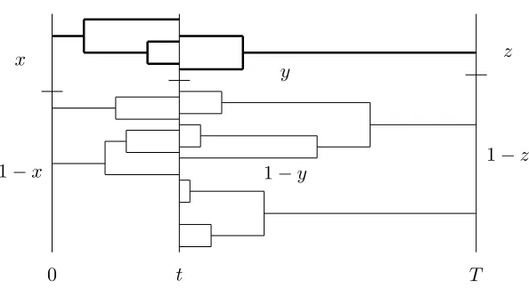
Figure 1: Genealogy in a neutral (0,0) bridge
x
1−x
z
1−z y
1−y
0 t T
There must be exactly 1 lineage from 0 totand fromT totin reverse time with leaves in the frequencyy, conditional ony being reached as x, z →0.
The description of the coalescent genealogy in the bridge is new in this paper and important. Informally the bridge density (16) timesdyis propor-tional to the proportion of sample paths in (y, y+dy) at a given time where the allele of frequencyy has a single ancestor in both directions at times t and T −t, divided by the proportion of sample paths in (y, y+dy), which is the speed measurey−1(1−y)−1.
It is of interest to consider the coalescent genealogy at time points s < t < T and calculate the number of lineages b, at T, which are non-mutant back to t, but not as far back as s; the number of non-mutant lineages a back to time s; and the number of distinct non-mutant lineages c back to times. To begin condition on the number of non-mutant lineages fromstot Lθ(t−s) =l. Then, from the representation at timet, considering the roots of the lineages fromT back tot, it must be that a fall on frequencies from VU and b fall on the frequencies (1−V){w(j)}. Therefore the conditional probability is
a+b a
EVa(1−V)b=
a+b a
l
(a)θ(b)
(l+θ)(a+b)
.
probability is therefore
X
a≥c
qa+b(T−t)
a+b a
EVa(1−V)b
l c
X
a;aj≥1 a! a1!· · ·ac!E
Ua1
1 · · ·Ucac
.
(17) Now
EU1a1· · ·Ucac
= a1!· · ·ac! l(a)
,
so the sum (17) is equal to
X
a≥c
qa+b(T −t)
a+b a
l
(a)θ(b)
(l+θ)(a+b)
· a!
l(a)
a−1 c−1
. (18)
The marginal distribution ofc from (18) is, settingm=a+b,
l c X m≥c
qm(T −t)
X
a
m! (m−a)!
θ(m−a)
(l+θ)(m)
a−1 c−1
. (19)
The inner sum of (19) is equal to
m(1 +θ)(m−1)
(l+θ)(m) X
a
m−1 a−1
a−1 c−1
1
(a−1)θ(m−1−(a−1))
(1 +θ)(m−1)
(20)
which is the coefficient ofuc−1 in
m(1 +θ)(m−1)
(l+θ)(m)
X
a≥1
m−1 a−1
(1 +u)a−1Eξa−1(1−ξ)m−1−(a−1) (21)
whereξ has a Beta (1, θ) distribution. Now (21) evaluates to
m(1 +θ)(m−1)
(l+θ)(m)
E(1 +uξ)m−1
showing that (21) is equal to
m(1 +θ)(m−1)
(l+θ)(m)
m−1 c−1
(c−1)! (1 +θ)(c−1)
.
Finally
P(Lθ(T−s) =c|Lθ(t−s) =l)
= l c X m≥c
qθm(T −t) m! (m−c)!
Γ(θ+m)
From (22) an identity also follows that
qcθ(T−s) =X l
qlθ(t−s)
l c
X
m≥c
qθm(T −t) m! (m−c)!
Γ(θ+m) Γ(θ+c)(l+θ)(m).
We now consider a bridge from 0 to 0 frequency when there is mutation away from a gene of typeA. The importance of this bridge is that it models a new mutant in the infinitely-many-alleles model which arises at time 0, then is lost at time T with mutation away from the new mutant to other types at rate θ/2. The generator for the frequency of a given allele in a neutral model is
L= 1
2x(1−x) ∂2 ∂x2 −
1 2θx
∂ ∂x.
The speed measure density is y−1(1−y)θ−1 and the process is reversible with respect to this measure before absorption. Theorem 1 holds for this model. Again care is needed for a 0,0 bridge. Asx→0
f0,θ(x, y;t) =x
∞
X
l=1
qθl(t)l(l+θ−1)(1−y)l+θ−2+o(x2)
and
f0,θ(y,0;t) = ∞
X
l=1
qlθ(t)l(l+θ−1)y(1−y)l−2.
Denote
gθ(y;t) = ∞
X
l=1
l(l+θ−1)(1−y)l+θ−2qθl(t). (23)
A similar calculation to that in Theorem 2, substituting in the second line of (11) gives the bridge density at t.
Theorem 3. The density of X0,0,[0,T](t), 0 ≤ t ≤ T in a neutral Wright-Fisher diffusion bridge with mutation away fromA at rateθ/2 is
y(1−y)−θ+1gθ(y;t)gθ(y;T −t)
P∞
l=1e−l(l+θ−1)T /2(2l+θ−1)l(l+θ−1)
. (24)
at 0 and T which have families in the y frequency. Theorem 2 and the coalescent interpretation are new.
The mean frequency in a bridge is found by multiplying (24) by y and integrating over (0,1).
Corollary 1.
EX0,0,[0,T](t)=
P∞
l,m=1
l(l+θ−1)m(m+θ−1)
(l+m+θ−2)(l+m+θ−3)qlθ(t)qθm(T −t)
P∞
l=1e−l(l+θ−1)T /2(2l+θ−1) (l−1)(l+θ) + 1 .
An algorithm to simulate exactly from the density in a neutral Wright-Fisher bridge is given in the Appendix.
3.2. h-transform identities for bridges
There are useful and interesting identities for bridge densities that follow from h-transforms. The transforms relate neutral Wright-Fisher transition functions when one or both of θ1, θ2 are zero to Wright-Fisher transition
functions with recurrent mutation whenθ1, θ2 >0. The bridge distribution
is invariant under theh-transform. Bridges beginning at 0 are easier to deal with after the transformation when beginning at zero, because the Wright-Fisher transition function is then well defined.
Supposeθ1 = 0, θ2 = 0, then an identity is
f2,2(x, y;t) =etf0,0(x, y;t)y(1−y)/x(1−x). (25)
To show the identity (25) consider the following calculation with the back-ward generator.
∂
∂tf2,2 = f2,2+e
ty(1−y) x(1−x) ·
1
2x(1−x) ∂2 ∂x2f0,0
= f2,2+
1 2
∂2
∂x2x(1−x)f2,2
= 1
2x(1−x) ∂2 ∂x2f2,2+
1
2(2−4x) ∂ ∂xf2,2.
This shows that the generator in theh-transformed process is
1
2x(1−x) ∂2
∂x2 +
1
2(2−4x) ∂ ∂x,
which corresponds to a Wright-Fisher diffusion with θ1 = θ2 = 2. The
also underh(x, t) =etx(1−x). This choice ofh(x, t) is made becausex(1−x) is the first eigenfunction and the first eigenvalue is 1.
There is a h-transform identity similar to (25) when θ1 = 0, θ2 =θ >0
where
f2,θ(x, y;t) =eθt/2f0,θ(x, y;t)y/x. (26)
A straightforward calculation is that
∂ ∂tf2,θ =
1
2x(1−x) ∂2 ∂x2f2,θ +
1
2 2−(2 +θ)x
∂
∂xf2,θ.
This shows that the generator in theh-transformed process is
1
2x(1−x) ∂2 ∂x2 +
1
2(2−(2 +θ)x) ∂ ∂x,
which corresponds to a Wright-Fisher diffusion with θ1 = 2, θ2 = θ. The
first eigenfunction in the process isx and first eigenvalueθ/2.
Corollary 2. An alternative form for the density ofXx,z,[0,T](t) in a neutral model whenθ1=θ2 = 0, for 0≤x, z ≤1 is
fx,z,[0,T](y;t) =
f2,2(x, y;t)f2,2(y, z;T −t)
f2,2(x, z;T)
= f2,2(z, y;T −t)f2,2(y, x;t) f2,2(z, x;T)
= fz,x,[0,T](y;T −t). (27)
An alternative form whenθ1 = 0, θ2=θ >0 0≤x, z ≤1 is
fx,z,[0,T](y;t) =
f2,θ(x, y;t)f2,θ(y, z;T −t) f2,θ(x, z;T)
= f2,θ(z, y;T −t)f2,θ(y, x;t) f2,θ(z, x;T)
= fz,x,[0,T](y;T −t). (28)
The densities on the right of these expressions are well defined at the boundaries whenx, z∈ {0,1} because of non-zero recurrent mutation rates. Notice that the two alternative forms of the bridge density (27) and (28) are not continuous inθatθ= 0.
Corollary 3. The limit density of Xx,z,[0,T](T /2 +t), θ1 = 0, θ2 = 0 as
T → ∞ is independent of tand is
6y(1−y), 0< y <1. (29)
for 0≤x, z≤1.
Corollary 4. The limit density of Xx,z,[0,T](T /2 +t), θ > 0 as T → ∞ is independent oftand is
θy(1−y)θ−1, 0< y <1. (30)
for 0≤x, z≤1.
The density (27) in Corollary 2 gives an alternative expression to (16) by settingx=z= 0, noting that terms on the right side are well defined in this case.
Other identities for the coalescent transition functions follow. Letting x→0 in the identity (25), using (6)
∞
X
r=0
qr4(t)(r+ 3)(r+ 2)y(1−y)r+1 =ety(1−y) ∞
X
r=2
r(r−1)qr0(t)(1−y)r−2,(31)
and equating coefficients ofy(1−y)l−1 shows the identity
(l+ 1)ql−4 2(t) =et(l−1)q0l(t). (32)
Another identity from the spectral expansion (3), and (25), equating coeffi-cients ofe−12n(n+4−1)t, is that forn≥0,
x(1−x)Pen(1,1)(r) =Pe (−1,−1)
n+2 (r). (33)
Letting x→0 in the identity (26) with θ1 = 0, θ2 =θ >0
∞
X
r=0
q2+r θ(t)(r+ 1 +θ)(r+θ)y(1−y)r+θ−1
=eθt/2y ∞
X
l=2
l(l+θ−1)qlθ(t)(1−y)l+θ−2
and equating coefficients ofy(1−y)l+θ−2 shows the identity
Also from (3) and (26)
xPen(θ−1,1)(r) =
n+ 1 n+θPe
(θ−1,−1)
n+1 (r). (35)
There is interest in the way the h-transforms are used to show the pairs of identities (32), (34) and (33) and (35). The first set is new, but probably not the second as so much is already known about Jacobi polynomials. The h-transform method of proof is new.
3.3. Wright-Fisher bridges and branching P´olya urns
A new representation of neutral Wright-Fisher bridges that come from Polya urns is now detailed. This has interest as a very classical probabilistic con-nection.
Genealogy in the Wright-Fisher diffusion process can be modelled by branching P´olya urns (Griffiths and Span`o, 2010). The joint density of X =X(0) and Y =X(t) when the marginal density ofX is Beta (θ1, θ2),
from the conditional density ofY given X, (6), can be written as
∞
X
l=0
qlθ(t) l
X
k=0
l k
θ
1(k)θ2(l−k)
θ(l)
Bk+θ1,l−k+θ2(x)Bk+θ1,l−k+θ2(y). (36)
There is a P´olya urn interpretation of (36), explained in Griffiths and Span`o (2010); Griffiths and Span`o (2013). Consider two P´olya urns with an ini-tial configuration of θ1 red andθ2 blue balls. The urns are identical until
there arelextra balls, then branch to two urns with probability qlθ(t). The composition of both urns at the moment of splitting has a Beta binomial distribution
l k
θ
1(k)θ2(l−k)
θ(l)
, k= 0,1, . . . , l.
Draws continue independently in each urn after branching. The uncondi-tional relative frequencies of red balls in the urns after an infinity of draws are Beta (θ1, θ2) and the relative frequencies conditional on a configuration
of (k, l−k) are Beta (θ1+k, θ2+l−k). In both cases the relative frequency
are red or blue, the probability of a configuration of (k, l−k) balls given the urns branch afterldraws and X=x is kl
xk(1−x)l−k. the distribution of Y given the (k, l−k) configuration is then Beta (θ1+l, θ2+l−k).
There-fore the conditional distribution of Y given X =x is (6). The conditional densityfθ1,θ2(x, y;t) converges asθ1, θ2 →0 to
f0,0(x, y;t) =
∞
X
l=1
q0l(t) l−1 X k=1 l k
xk(1−x)l−kBk,l−k(y). (37)
Relating the limit to convergence in an urn model: ifl >1 the conditional distribution of the urn configuration atl given 0< x <1 as θ1, θ2 →0 is
l k
xk(1−x)l−k, 0< k < l
as a consequence of the de Finetti representation. The joint probability that k = 0 (and similarly for k = l) at trial l and 0 < x < 1 tends to zero as θ1, θ2 →0, even though it formally appears to be (1−x)l.
We now give a new interpretation of Wright-Fisher bridges in terms of an urn model with three urns. In a neutral Wright-Fisher diffusion with mutation the density of the frequency at timetin a bridge fromxtozat time tis (8), where fθ1,θ2(x, y;t) is the density (2) or (6). An urn representation is found by considering the joint distribution of X, Y, Z when X and Z have marginal Beta (θ1, θ2) distributions. The joint distribution of the three
random variables is then
Bθ1,θ2(x)fθ1,θ2(x, y;t)fθ1,θ2(y, z;T −t)
= ∞
X
l,m=0
qθl(t)qmθ(T−t) X j≤l,k≤m
n j+k
θ
1(j+k)θ2(n−j−k)
θ(n)
l j m k n j+k
× Bθ1+j,θ2+l−j(x)Bθ1+k,θ2+m−k(z)Bθ1+k+j,θ2+n−k−j(y), (38)
where n = l +m. An urn representation has three urns U, V, W which share draws before branching after drawninW. The probability of branch-ing after n draws and that there are l, m draws respectively in U, V is ql(t)qm(T −t). The l, m draws are chosen at random from the n draws. After branching the urn draws continue independently inU, V, W. For fixed l, m the probability of configurations (j, l−j) and (k, m−k) of (red,blue) balls in urns U, V and (j+k, n−j−k) in urnW is
n j+k
θ
1(j+k)θ2(n−j−k)
θ(n)
l j m k n j+k
Conditional onl, m, j, kthe limit relative frequencies of red balls inU, V, W have the joint density in the last line of (38). The unconditional joint density of the relative frequencies in urnsU, V, W is the full expression (38).
The configuration in the urns at branching, conditional onX=x, Z=z has a probability distribution
pθ1,θ2(l, m;j, k;x, z;t) =
qlθ(t)qmθ(T−t) j+nkθ1(j+k)θ2(n−j−k) θ(n)
(l j)(
m k) ( n
j+k)
Bθ1+j,θ2+l−j(x)Bθ1+k,θ2+m−k(z)
Bθ1,θ2(x)fθ1,θ2(x, z;T)
.
(39)
Then forl, m≥1 as θ1, θ2→0 the distribution (39) converges to
p0,0(l, m;j, k;x, z;t) =
q0l(t)qm0(T−t) j+nk(j+k−1)!((n−n−j−k−1)! 1)!( l j)(
m k) ( n
j+k)
Bj,l−j(x)Bk,m−k(z)
x−1(1−x)−1f
0,0(x, z;T)
.
(40)
There is a similar limit ifθ1 → 0 andθ2 >0. The relative frequency of red
balls in urnW after an infinite number of draws whenθ1, θ2 >0 has a Beta
(θ1+j+k, θ2+n−j−k) distribution so the density of Y conditional on
X=x, Z =z is
∞
X
l,m=0
pθ1,θ2(l, m;j, k;x, z;t)Bθ1+j+k,θ2+n−j−k(y), (41)
with a similar expression when θ1 = 0, θ2 = 0 where summation is over
l, m ≥ 1, 1 ≤ j ≤ l−1 and 1 ≤ k ≤ m−1. The density (41) is the same as the neutral bridge densities in Section 3.1 with the different cases of mutation. The limit distribution whenθ1 = 0, θ2 = 0 andx, z→0 is now
considered. The denominator of (40) converges to
∞
X
l=1
q0l(T)l(l−1)
configurations (40) converges to zero unlessj= 1, k= 1 when the limit is
p0,0(l, m;j, k; 0,0;t) =
ql0(t)q0m(T −t) n21!((n−n−1)!3)! lm (n
2)
(l−1)(m−1)
P∞
l=2e
−1
2l(l−1)T(2l−1)(l−1)
= q
0
l(t)q0m(T −t)
l(l−1)m(m−1) (n−1)(n−2) P∞
l=2e
−1
2l(l−1)T(2l−1)(l−1) .
The conditional distribution of the relative frequency of red balls in urnW is then
∞
X
n=2
X
l,m≥1,l+m=n
p0,0(l, m;j, k; 0,0;t)B2,n−2(y).
3.4. Wright-Fisher bridges with genic selection
In this section we consider the genealogy of a Wright-Fisher bridge when there is selection in the model. This is a new approach different from that in Schraiber et. al. (2013). The genealogy of the Wright-Fisher diffusion with selection is more complex that in a neutral model and the transition functions for the coalescent genealogy do not have an explict form.
Theorem 1 holds when γ 6= 0, if x 6= 0, however care is again needed when beginning from x = 0. For definiteness let γ > 0, then the speed measure density whenθ1 = 0 and θ2 =θ≥0 is
eγxx−1(1−x)θ−1, 0< x <1.
The density is reversible before fixation and withθ= (0, θ),
f0,θ,γ(x, y;t) = X
α
b(0α,θ)(t, x)π[α+θ](y)
= X
α
b(0α,θ)(t, y)π[α+θ](x)
y−1(1−y)θ−1eγy
x−1(1−x)θ−1eγx. (42)
αi ≥1 in the summation,i= 1,2. In a neutral model
b(0α,θ)(t, y) =
|
α|
α1
yα1(1−y)α2
An asymptotic form asx→0 is
f0,θ,γ(x, y;t) =y−1(1−y)θ−1eγyx
X
α2≥1 b(0(1,θ,α)
2+θ)(t, y)(α2+θ)c(1, α2+θ)
sinceπ[α+θ](x) =o(xα1−1) as x→0 forα
1>1 and
π[(1, α2+θ)](x) =c(1, α2+θ)−1
Γ(1 +α2+θ)
Γ(1)Γ(α2+θ)
x1−1(1−x)α2+θ−1eγx.
Note that
c(1, α2+θ) = Z 1
0
(α2+θ)zα2+θ−1ezγdz, γ ≥0.
Denote
gθ(y;t;γ) =y−1(1−y)θ−1eγy ∞
X
α2=1 b(0(1,θ,α)
2)(t, y)(α2+θ)c(1, α2+θ) −1.
We have shown that asx→0
f0,θ,γ(x, y;t) =xgθ(y;t;γ) +o(x2)
and that
f0,θ,γ(y,0;t) =y(1−y)1−θe−γygθ(y;t;γ).
The next theorem is an analogue of Theorem 2 which follows by substitution in the second line of the bridge density (11) and the asymptotic forms in this section for the transition density.
Theorem 4. The density of X0,0,[0,T](t), 0 ≤ t ≤ T in a Wright-Fisher diffusion bridge whenγ >0 with mutation away from Aat rate θ/2≥0 is
y(1−y)1−θe−γygθ(y;t, γ)gθ(y;T −t, γ)
P∞
α2=1b 0(0,θ)
(1,α2)(T,0)c(1, α2+θ) −1(α
2+θ)
,
where prime denotes differentiation with respect toy.
Figure 4: Genealogy in a non-neutral (0,0) bridge
y
1−y
0 t T
We are interested in finding the Yaglom density and the limit distribution ofXx,z,[0,T](T /2+t) asT → ∞. These calculations depend on the first eigen-functionw(y). The Yaglom density is proportional toy−1(1−y)θ−1eγyw(y). An analogy of theh-transform (25) in the non-neutral model is
fw(x, y;t) =f(x, y;t)w(y) w(x)e
λt,
where (λ, w) are the first eigenvalue, eigenfunction pair satisfying (7) when either or both ofθ1, θ2 are zero. A calculation similar to that in the neutral
model shows that the generator associated with the transition functionsfw whenθ1 = 0, θ2 =θ≥0 is
1
2x(1−x) ∂2 ∂x2 +
1
2 γx(1−x) + 2x(1−x) ∂
∂xlogw(x)−θx
!
∂
∂x. (43)
This is a generator of a Wright-Fisher diffusion with frequency dependent selection. The stationary distribution of the process with generator (43) is
ψ(y) =Cw(y)2π(y) =Cw(y)2eγyy−1(1−y)θ−1.
An alternative form for the density ofXx,z,[0,T] is, for 0≤t≤T
fw(x, y;t)fw(y, z;T −t)
fw(x, z;T) . (44)
The limit density asT → ∞ of Xx,z,[0,T](T /2 +t), from (44) is
Computing ψ(y) (when θ = 0) rests on finding a numerical solution of the eigenfunction equation
y(1−y)w00(y) +γy(1−y)w0(y) + 2λw(y) = 0
for a maximalλ. There is a unique solution withλ > 0, w(x)≥0. Clearly w(0) =w(1) = 0 but the maximalλ is unknown. Parameterizingλ≡λ(γ), then λ(0) = 1, the first eigenvalue in a neutral model. Kimura (1955) recognizes a connection with Spheroidal wave functions, tabulatesλ(γ), and expressesw(x) as a series in Gegenbauer polynomials. The spheroidal wave equations are
d dz
(1−z2)dS dz
+
µ+c2(1−z2)− m
2
1−z2
S = 0, (45)
see NIST Handbook of Mathematical Functions (2010). Ifc2 >0 the equa-tions areprolate orc2 <0oblate. Solutions to (45) are the Spheroidal wave
functionsPSm n(z, c
2) with eigenvaluesµm
n(c2),n=m, m+ 1, . . .. Letting
w(y) =e−(γ/2)yy1/2(1−y)1/2S◦(y),
then
d dy
y(1−y)dS ◦
dy
+
µ−c2+ 4c2y(1−y)− m
2
4y(1−y)
S◦ = 0.
This shows that eγ/2yy−1/2(1 −y)−1/2w(y) is proportional to PS1 1(2y − 1),−γ2/16). Parameters are m = 1, c2 = −γ2/16, and µ−c2 = 2λ and z= 1−2y. Scalingw(y) to be a probability distribution
w(y) = e
−γ/2yy1/2(1−y)1/2P
S1
1(2y−1,−γ
2/16)
R1
0 e−(γ/2)xx1/2(1−x)1/2PS1
1(2x−1,−γ
2/16)dx.
Spheroidal wave functions are implemented in Mathematica and it is straight-forward to calculate and plot w(y) via WolframAlpha on a web interface. The basic command for solutions to (45) isSpheroidalPS[n,m,c,z]. In our applicationc2 ≤0 so c is a multiple of the complex numberi. For example
ifγ = 3, thenc= 0.75i, and n=m= 1,
is the appropriate command. The constant−0.166599 is the scaling factor returned by
Integrate[exp(-1.5*x)(x*(1-x))^(1/2) *SpheroidalPS[1,1,0.75i,2*x -1],{x,0,1}]
It is not necessary to find the first eigenvalue for the above commands, however SpheroidalEigenvalue[n,m,c] will return it. In this example
Eigenvalue[1,1,0.75i]returns 2.44853, soλ= 1.505515. The full
expan-sion of the transition function is
f0,0,γ(x, y;t) =eγyy−1(1−y)−1 ∞
X
n=1
e−(λ1n( γ2 16)+
γ2 16)
t
2 2n+ 1 n(n+ 1)
×e−γ2xx 1
2(1−x) 1 2P
S1
n(2x−1,− γ2 16)
×e−γ2yy 1
2(1−y) 1 2PS1
n(2y−1,− γ2 16).
This expansion is analogous to the neutral expansion (4). Mathematica also includes a function for the derivative of a Spheroidal wave function,
SpheroidalPSPrime[n,m,c,z]. The drift coefficient in the h-transformed
generator (43) when θ = 0 can thus be easily evaluated or plotted. The coefficient is easily seen to be
1
2(1−2x) + 2x(1−x) PS01
1
(2x−1,−γ2/16)
PS1
1(2x−1,−γ
2/16).
Carrying through the example above, if γ = 3, the command to plot the drift coefficient is
Plot[0.5-x +2.0*x*(1-x)*SpheroidalPSPrime[1,1,0.75i,2*x-1] /SpheroidalPS[1,1,0.75i,2*x-1],{x,0,1}]
In this particular example the the plot shows that the drift coefficient is very close to 1−2x, which would be exact ifγ = 0 andw(x) =x(1−x).
Appendix: Simulating the neutral Wright-Fisher bridge
It is possible to simulate exactly from the density of a Wright-Fisher bridge in a neutral model. We develop a new algorithm here when one or both of x, z are zero. Jenkins and Span`o (2017) gave a sophisticated algorithm for this in the special case that both θ1, θ2 >0 and x, z >0. The identities in
1. θ1 = 0,θ2 =θ >0, andx=z= 0.
2. θ1 =θ2 = 0 andx=z= 0.
3. θ1 = 0,θ2 =θ >0, andx, z >0.
4. θ1 =θ2 = 0 andx, z >0.
1. θ1 = 0, θ2 =θ >0 and x=z= 0
The density ofX0,0,[0,T](t) is given in Theorem 3. It can be written as
f0,0,[0,T](t) = ∞
X
l1=1 ∞
X
l2=1 pl1,l2
y(1−y)l1+l2+θ−3 B(2, l1+l2+θ−2)
, (46)
where
pl1,l2 = 1 hθ(T)
l1(l1+θ−1)l2(l2+θ−1)
(l1+l2+θ−1)(l1+l2+θ−2)
qlθ1(t)qlθ2(T −t),
hθ(T) =gθ(0;T) = ∞
X
l=1
e−l(l+θ−1)T /2(2l+θ−1)l(l+θ−1).
We recognise (46) as the density of an infinite mixture of Beta random variables, so that (pl1,l2)l1,l2∈N is a probability mass function on N
2 (for
convenience, set pl1,l2 = 0 if l1 = 0 or l2 = 0). The (l1, l2)th component corresponds to a Beta(2, l1+l2+θ−2) variate. Therefore in order to simulate
fromf0,0,[0,T](t), it suffices to simulate from the discrete distribution (pl1,l2). This is complicated by the infinite series representations forqθl1(t),qlθ2(T−t), and hθ(T), but a solution is possible via the series method (Devroye, 1986, Ch. IV.5); we summarise the strategy as follows.
Suppose (pl)l∈Nis a probability mass function whose masses may not be computable with finite resource but for which we have available a pair of sequences (p−l (k))k∈N, (p+l (k))k∈N for each lwith the following properties:
1. p−l (k)≤pl ≤p+l (k) for all l, k∈N.
2. For eachl,p−l (k)↑pl ask→ ∞.
ForU ∼Uniform[0,1], standard inversion sampling implies that inf{L∈N:
PL
l=0pl > U} is distributed according to (pl), but this is not computable, as we have noted. However, it is easily verified that if
K(L) = inf
(
k∈N:
L
X
l=0
p−l (k)> U or L
X
l=0
p+l (k)< U
)
then
inf
(
L∈N: L
X
l=0
p−l (K(l))> U
)
is also distributed as (pl), and this can be computed from finitely many terms in the double arrays (p−l (k)), (p+l (k)).
To employ this strategy for (pl1,l2) in (46) we must find monotonically converging upper and lower bounds on each ofqθl1(t),qlθ2(T−t), andhθ(T). The first two expressions are covered by Jenkins and Span`o (2017, Proposi-tion 1), who showed that
(qθ)−l (k, t) := l+2k+1
X
j=l
ρθj(t)(−1)j−l(2j+θ−1)(l+θ)j−1 l!(j−l)! ≤q
θ l(t)
≤
l+2k
X
j=l
ρθj(t)(−1)j−l(2j+θ−1)(l+θ)j−1 l!(j−l)! =: (q
θ)+
l (k, t),
provided 2k+l≥Cl(t,θ):= inf
n
i≥l: θ+i−li++1l−1θθ+2+2ii−+11e−(i+θ/2)t<1
o
, a con-stant beyond which convergence of these bounds becomes monotonic in k. Jenkins and Span`o (2017) assumed thatθ1, θ2 > 0, but their result follows
without change when either or both of θ1 = 0, θ2 = 0.] It remains to find
similar converging bounds on hθ(T). Writing
hθ(T) = ∞
X
l=1
e−l(l+θ−1)T /2(2l+θ−1)l(l+θ−1) =: ∞
X
l=1
hθl(T),
we find for l≥2 that
hθl+1(T) = (2l+ 1 +θ)(l+ 1)(l+θ) (2l−1 +θ)(l−1)(l+θ−1)e
−(l+θ/2)Thθ
l(T)≤5e−(l+θ/2)Thθl(T)< hθl(T),
with the final inequality holding providedl > D(θ,T):= log 5T −θ2. It follows immediately that, fork >max(2, D(θ,T)),
0< ∞
X
l=k
hθl(T)≤
∞
X
l=k
and hence that
h−k(T) := k
X
l=1
e−l(l+θ−1)T /2(2l+θ−1)l(l+θ−1),
h+k(T) := h−k(T) + h θ k+1(T)
1−5e−(k+1+θ/2)T
serve as monotonically converging lower and upper bounds on hθ(T) as k→ ∞. We summarise the above argument in the following result.
Theorem 5. Let Σ :N→N2 be any bijective pairing function denoted by
Σ(l) = (l1, l2), and let
Sk−(L) =
Σ(L) X
l=Σ(0)
l1(l1+θ−1)l2(l2+θ−1)
(l1+l2+θ−1)(l1+l2+θ−2)
(qθ)−l
1(kl, t)(q θ)−
l2(kl, T −t) h+k
l(T)
,
Sk+(L) =
Σ(L) X
l=Σ(0)
l1(l1+θ−1)l2(l2+θ−1)
(l1+l2+θ−1)(l1+l2+θ−2)
(qθ)+l
1(kl, t)(q θ)+
l2(kl, T −t) h−k
l(T)
.
Ifkl>max
(Cl(t)
1 −l1)/2,(C
(T−t)
l2 −l2)/2, D
(T ,θ),2for eachl= 0,1, . . . , L,
then Sk−(L) and Sk+(L) are respectively lower and upper bounds on the
distribution function PΣ(l=Σ(0)L) pl1,l2 which are monotonically converging to this limit as k → ∞ (that is, as kl → ∞ for every component of k = (k0, k1, . . . , kL)). Thus the following algorithm returns exact samples from
Algorithm 1: Simulating from the densityf0,0,[0,T](t) ofX0,0,[0,T](t) when θ1= 0, θ2=θ >0.
1 Setl←−0,k0←−0,k←−(k0).
2 Simulate U ∼Uniform[0,1]. 3 repeat
4 Set (l1, l2)←−Σ(l),
kl←−
l
max(Cl(t)
1 −l1)/2,(C
(T−t)
l2 −l2)/2, D
(T,θ),2m.
5 while Sk−(l)< U < Sk+(l) do 6 Set k←−k+ (1,1, . . . ,1).
7 end
8
9 if Sk−(l)> U then
10 return Y ∼Beta(2, l1+l2+θ−2). 11 else if Sk+(l)< U then
12 Set k←−(k0, k1, . . . , kl,0).
13 Set l←−l+ 1.
14 end
15 until false
2. θ1 =θ2 = 0 and x=z= 0
This case is very similar to that of the previous subsection and so is omitted. (In fact, one can go through the previous subsection and replace θ with 0 throughout.) The density of the bridge whenθ1 =θ2 = 0 simplifies slightly
(see Theorem 2) to
f0,0,[0,T](t) = ∞
X
l1=2 ∞
X
l2=2 pl1,l2
y(1−y)l1+l2−3 B(2, l1+l2−2)
,
pl1,l2 = 1 h(T)
l1(l1−1)l2(l2−1)
(l1+l2−1)(l1+l2−2)
ql01(t)ql02(T −t).
3. θ1 = 0, θ2 =θ >0 and x, z >0
By Corollary 2, the density of Xx,z,[0,T](t) in this case is the same as for θ1 = 2, θ2 = θ, which is covered by Algorithm 4 of Jenkins and Span`o
4. θ1 =θ2 = 0 and x, z >0
By Corollary 2, the density of Xx,z,[0,T](t) in this case is the same as for θ1 =θ2 = 2, which is covered by Algorithm 4 of Jenkins and Span`o (2017).
References
Barbour, A.D., Ethier, S.N., Griffiths, R.C. (2000). A transition function expansion for a diffusion model with selection. Ann. Appl. Probab. 10, 123–162.
Devroye, L. (1986). Non-uniform random variate generation. Springer-Verlag, New York.
Etheridge, A. M., Griffiths, R. C. (2009). A coalescent dual process in a Moran model with genic selection. Theor. Popul. Biol. 75, 320–330.
Ethier, S. and Griffiths, R. C. (1993). The transition function of a Fleming-Viot process. Ann. Probab. 21, 1571–1590.
Fitzsimmons, P., Pitman, J., Yor, M. (1992). Markovian bridges: construc-tion, Palm interpretaconstruc-tion, and splicing. Seminar on stochastic processes, Progress in probability, 33, 101–134, ed. C¸ inlar, E. Chung, K. L., Sharpe. M. J. , Bass, R. F., Burdzy, K., Birkh¨auser, Boston.
Griffiths, R.C., (1980). Lines of descent in the diffusion approximation of neutral Wright-Fisher models. Theor. Popul. Biol. 17, 37–50.
Griffiths, R. C. (1984). Asymptotic line-of-descent distributions. J. Math. Biol. 21, 67–75.
Griffiths, R.C. and Tavar´e, S. (1998). The age of a mutation in a general coalescent tree. Stochastic Models. 14, 273–295.
Griffiths, R.C. and Tavar´e, S. (2003). The genealogy of a neutral mutation. In: Green, P.J., Hjort, N.L. and Richardson, S. (Eds.), Highly Structured Stochastic Systems. Oxford University Press, Oxford, pp. 393–413.
Griffiths, R.C. (2006). Coalescent lineage distributions. Adv. Appl. Probab. 38, 405–429.
Griffiths, R. C. and Span`o, D. (2010). Diffusion processes and coalescent trees. Chapter 15 358-375. In: Probability and Mathematical Genetics, Papers in Honour of Sir John Kingman. LMS Lecture Note Series 378. ed Bingham, N. H. and Goldie, C. M., Cambridge University Press.
Griffiths, R. C. and Span`o (2013), D. Orthogonal Polynomial Kernels and Canonical Correlations for Dirichlet measures, Bernoulli 19, 548–598.
Ismail, M.E.H. (2005) Classical and quantum orthogonal polynomials in one variable. Cambridge University press. Cambridge UK.
Jenkins, P. A. and Span`o, D. (2017) Exact simulation of the Wright-Fisher diffusion. Ann. Appl. Prob. 27, 1478–1509.
Kimura, M. (1955) Stochastic processes and distribution of gene frequencies under natural selection. Cold Spring Harb. Symp. Quant. Biol. 20, 33–53.
Kimura, M. (1957) Some problems of stochastic processes in genetics. Ann. Math. Stat. 28, 882–901.
Kimura, M. (1964). Diffusion models in population genetics. J. Appl. Prob. 1, 177–232.
Kingman, J.F.C. (1982). The coalescent. Stochastic Process. Appl. 13, 235– 248.
Krone, S. M., Neuhauser, C. (1997). Ancestral processes with selection. Theor. Popul. Biol. 51, 210–237.
Mano, S., (2009). Duality, ancestral and diffusion Processes in models with selection. Theor. Popul. Biol. 75, 164–175.
Neuhauser, C., Krone, S. M. (1997). The genealogy of samples in models with selection. Genetics 145, 519–534.
NIST Handbook of Mathematical Functions (2010). Editors: F. W. J. Olver, D. W. Lozier R. F. Boisvert C. W. Clark. Cambridge University Press, New York.
Pinsky, R.G. (1985). On the convergence of diffusion processes conditioned to remain in a bounded region for large time to limiting positive recurrent diffusion processes. Ann. Prob. 13, 363–378.
Schraiber, J. Griffiths, R. C., Evans, S. (2013). Analysis and rejection sam-pling of Wright-Fisher diffusion bridges. Theor. Popul. Biol. 89, 64–74.
Song, Y.S., Steinr¨ucken, M. (2012). A simple method for finding explicit analytic transition densities of diffusion processes with general diploid selection. Genetics, 190, 1117–1129.
Steinr¨ucken, M., Wang, Y.X., and Song Y.S. (2013). An explicit transition density for a multi-allelic Wright-Fisher diffusion with general diploid se-lection. Theor. Popul. Biol. 83, 1–14.