warwick.ac.uk/lib-publications
Original citation:
Dunlop, Matthew M., Iglesias, Marco A. and Stuart, Andrew M.. (2016) Hierarchical Bayesian
level set inversion. Statistics and Computing.
Permanent WRAP URL:
http://wrap.warwick.ac.uk/86352
Copyright and reuse:
The Warwick Research Archive Portal (WRAP) makes this work by researchers of the
University of Warwick available open access under the following conditions. Copyright ©
and all moral rights to the version of the paper presented here belong to the individual
author(s) and/or other copyright owners. To the extent reasonable and practicable the
material made available in WRAP has been checked for eligibility before being made
available.
Copies of full items can be used for personal research or study, educational, or not-for profit
purposes without prior permission or charge. Provided that the authors, title and full
bibliographic details are credited, a hyperlink and/or URL is given for the original metadata
page and the content is not changed in any way.
Publisher’s statement:
“The final publication is available at Springer via
http://dx.doi.org/10.1007/s11222-016-9704-8
A note on versions:
The version presented here may differ from the published version or, version of record, if
you wish to cite this item you are advised to consult the publisher’s version. Please see the
‘permanent WRAP url’ above for details on accessing the published version and note that
access may require a subscription.
MATTHEW M. DUNLOP, MARCO A. IGLESIAS, AND ANDREW M. STUART
Abstract. The level set approach has proven widely successful in the study of inverse problems for interfaces, since its systematic development in the 1990s. Recently it has been employed in the context of Bayesian inversion, allowing for the quantification of uncertainty within the reconstruction of interfaces. However the Bayesian approach is very sensitive to the length and amplitude scales in the prior probabilistic model. This paper demonstrates how the scale-sensitivity can be circumvented by means of a hierarchical approach, using a single scalar parameter. Together with careful consideration of the development of algorithms which encode probability measure equivalences as the hierarchical parameter is varied, this leads to well-defined Gibbs based MCMC methods found by alternating Metropolis-Hastings updates of the level set function and the hierarchical parameter. These methods demonstrably outperform non-hierarchical Bayesian level set methods. Inverse problems for interfaces and Level set inversion and Hierarchical Bayesian methods
1. Introduction
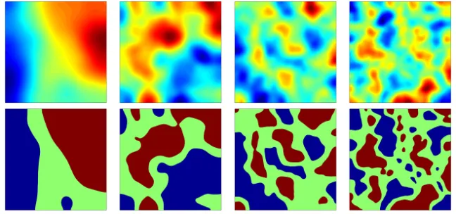
1.1. Background. The level set method has been pervasive as a tool for the study of interface problems since its introduction in the 1980s [43]. In a seminal paper in the 1990s, Santosa demonstrated the power of the approach for the study of inverse problems with unknown interfaces [47]. The key benefit of adopting the level set parametrization of interfaces is that topological changes are permitted. In particular for inverse problems the number of connected components of the field does not need to be known a priori. The idea is illustrated in Figure 1. The type of unknown functions that we might wish to reconstruct are piecewise continuous functions, illustrated in the bottom row by piecewise constant ternary functions. However in the inversion we work with a smooth function, shown in the top row and known as the level-set function, which is thresholded to create the desired unknown function in the bottom row. This allows the inversion to be performed on smooth functions, and allows for topological changes to be detected during the course of algorithms. After Santosa’s paper there were many subsequent papers employing the level set representation for classical inversion, and examples include [11, 15, 19, 52], and the references therein.
In many inverse problems arising in modern day science and engineering, the data is noisy and prior regularizing information is naturally expressed probabilistically since it contains uncertainties. In this context, Bayesian inversion is a very at-tractive conceptual approach [33]. Early adoption of the Bayesian approach within level set inversion, especially in the context of history matching for reservoir simu-lation, includes the papers [39, 40, 44, 56]. In a recent paper [31] the mathematical foundations of Bayesian level set inversion were developed, and a well-posedness theorem established, using the infinite dimensional Bayesian framework developed in [18, 34, 35, 51]. An ensemble Kalman filter method has also been applied in the
1
Figure 1. Four continuous scalar fields (top) and the correspond-ing ternary fields formed by thresholdcorrespond-ing these fields at two levels (bottom). The smooth function in the top row is known as the level-set functionand is used in the inversion procedure. The dis-continuous function in the bottom row is the physical unknown.
Bayesian level set setting [28] to produce estimates of piecewise constant permeabil-ities/conductivities in groundwater flow/electrical impedance tomography (EIT) models.
1.2. Key Contributions of the Paper. The key contribution of this paper is in computational statistics: we develop a Metropolis Hastings method with mesh-independent mixing properties that makes an order of magnitude of improvement in the Bayesian level set method as introduced in [31].
Study of Figure 1 suggests that the ability of the level set representation to accurately reconstruct piecewise continuous fields depends on two important scale parameters:
• the length-scale of the level set function, and its relation to the typical separation between discontinuities;
• the amplitude-scale of the level set function, and its relation to the levels used for thresholding.
If these two scale parameters are not set correctly then MCMC methods to de-termine the level set function from data can perform poorly. This immediately suggests the idea of using hierarchical Bayesian methods in which these parameters are learned from the data. However there is a second consideration which interacts with this discussion. From the work of Tierney [53] it is known that absolute conti-nuity of certain measures arising in the definition of Metropolis-Hastings methods is central to their well-definedness, and hence to discretization invariant MCMC methods [16]. In fact it appears algorithms defined on infinite dimensional spaces have spectral gaps that are bounded independently of the mesh, and so their con-vergence rates are bounded below in the limit [26]. The key contribution of our paper is to show how enforcing absolute continuity links the two scale parameters, and hence leads to the construction of a hierarchical Bayesian level set method with asingle scalarhierarchical parameter which deals with the scale and absolute continuity issues simultaneously, resulting in effective sampling algorithms.
The hierarchical parameter is an inverse length-scale within a Gaussian random field prior for the level set function. In order to preserve absolute continuity of different priors on the level set function as the length-scale parameter varies, and relatedly to make well-defined MCMC methods, the mean square amplitude of this Gaussian random field must decay proportionally to a power of the inverse length-scale. It is thus natural that the level values used for thresholding should obey this power law relationship with respect to the hierarchical parameter. As a consequence the likelihood depends on the hierarchical parameter, leading to a novel form of posterior distribution.
We construct this posterior distribution and demonstrate how to sample from it using a Metropolis-within-Gibbs algorithm which alternates between updating the level set function and the inverse length scale. As a second contribution of the paper, we demonstrate the applicability of the algorithm on three inverse problems, by means of simulation studies. The first concerns reconstruction of a ternary piecewise constant field from a finite noisy set of point measurements: in this context, the Bayesian level set method is very closely related to a spatial probit model [45]. This relation is discussed in in subsection 2.4. The other two concern reconstruction of the coefficient of a divergence form elliptic PDE from measurements of its solution; in particular, groundwater flow (in which measurements are made in the interior of the domain) and EIT (in which measurements are made on the boundary).
which remain absolutely continuous with respect to one another when we vary this parameter; we then place a hyper-prior on this parameter. We describe an appro-priate level set map, dependent on the length-scale parameter because length and amplitude scales are intimately connected through absolute continuity of measures, to transform these fields into piecewise constant ones, and use this level set map in the construction of the likelihood. We end by showing existence and well-posedness of the posterior distribution on the level set function and the inverse length scale parameter. In section 3 we describe a Metropolis-within-Gibbs MCMC algorithm for sampling the posterior distribution, taking advantage of existing state-of-the-art function space MCMC, and the absolute continuity of our prior distributions with respect to changes in the inverse length scale parameter, established in the previous section. Section 4 contains numerical experiments for three different for-ward models: a linear map comprising pointwise observations, groundwater flow and EIT; these illustrate the behavior of the algorithm and, in particular, demon-strate significant improvement with respect to non-hierarchical Bayesian level set inversion.
2. Construction of the Posterior
In subsection 2.1 we recall the definition of the Whittle-Mat´ern covariance func-tions, and define a related family of covariances parametrized by an inverse length scale parameterτ. We use these covariances to define our prior on the level set func-tionu, and also place a hyperprior on the parameterτ, yielding a priorP(u, τ) on a product space. In subsection 2.2 we construct the level set map, taking into account the amplitude scaling of prior samples withτ, and incorporate this into the forward map. The inverse problem is formulated, and the resulting likelihood P(y|u, τ) is
defined. Finally in subsection 2.3 we construct the posteriorP(u, τ|y) by combining
the priorP(u, τ) and likelihoodP(y|u, τ) using Bayes’ formula. Well-posedness of
this posterior is established.
2.1. Prior. As discussed in the introduction it can be important, within the con-text of Bayesian level set inversion, to attempt to learn the length-scale of the level set function whose level sets determine interfaces in piecewise continuous recon-structions. This is because we typically do not know a-priori the typical separation of interfaces. It is also computationally expedient to work with Gaussian random field priors for the level set function, as demonstrated in [20, 31]. A family of covariances parameterized by length scale is hence required.
A widely used family of distributions, allowing for control over sample regularity, amplitude and length scale, are Whittle-Mat´ern distributions. These are a family of stationary Gaussian distributions with covariance function
cσ,ν,`(x, y) =σ22 1−ν
Γ(ν)
|x−y|
` ν
Kν
|x−y|
`
stochastic partial differential equation (SPDE). This SPDE can be derived using the Fourier transform and the spectral representation of covariance functions – the paper [36] derives the appropriate SPDE for the covariance function above:
1
p
β`d(I−`
2
4)(ν+d/2)/2v=W
(1)
whereW is a white noise on Rd, and
β =σ22
dπd/2Γ(ν+d/2)
Γ(ν) .
Computationally, implementation of this SPDE approach requires restriction to a bounded subsetD ⊆Rd, and hence the provision of boundary conditions for the
SPDE in order to obtain a unique solution. Choice of these boundary conditions may significantly affect the autocorrelations near the boundary. The effects for dif-ferent boundary conditions are discussed in [36]. Nonetheless, the computational expediency of the SPDE formulation makes the approach very attractive for ap-plications and, if necessary, boundary effects can be ameliorated by generating the random fields on larger domains which are a superset of the domain of interest.
From (1) it can be seen that the covariance operator corresponding to the co-variance functioncσ,ν,`is given by
Dσ,ν,`=β`d(I−`24)−ν−d/2. (2)
The fact that the scalar multiplier in front of the covariance operatorDσ,ν,`changes with the length-scale means that the family of measures {N(0,Dσ,ν,`)}`, for fixed
σ and ν, are mutually singular. This leads to problems when trying to design hierarchical methods based around these priors. We hence work instead with the modified covariances
Cα,τ = (τ2I− 4)−α
where τ = 1/` >0 now represents an inverse length scale, and α=ν+d/2 still controls the sample regularity. To be concrete we will always assume that the domain of the Laplacian is chosen so that Cα,τ is well-defined for all τ ≥ 0; for example we may choose a periodic box, with domain restricted to functions which integrate to zero over the box, Neumann boundary conditions on a box, again with domain restricted to functions which integrate to zero over the box, or Dirichlet boundary conditions. We have the following theorem concerning the family of Gaussians{N(0,Cα,τ)}τ≥0, proved in the Appendix.
Theorem 2.1. Let D =Td be thed-dimensional torus, and fix α >0. Define the
family of Gaussian measuresµτ
0 =N(0,Cα,τ),τ≥0. Then (i) for d≤3, the {µτ
0}τ≥0 are mutually equivalent;
(ii) if u ∼ µτ
0, then µτ0-a.s. we have u ∈ Hs(D) and u ∈ Cbsc,s−bsc(D) for all s < α−d/2. 1
(iii) ifu∼µτ
0 andv∼N(0,Dσ,ν,`), then
Ekuk2∝τd−2α·Ekvk2
with constant of proportionality independent ofτ.
1i.e. the function hassweak (possibly fractional) derivatives in the Sobolev sense, and thebscth
Remark 2.2. (a) Proof of this theorem is driven by the smoothness of the eigen-functions of the Laplacian subject to periodic boundary conditions, together with the growth of the eigenvalues, which is like j2/d. These properties extend to Laplacians on more general domains and with more general boundary condi-tions, and to Laplacians with lower order perturbacondi-tions, and so the above result still holds in these cases. For discussion of this in relation to (ii) see [18]; for parts (i) and (iii) the reader can readily extend the proof given in the Appendix.
(b) The proportionality in part (iii) above could be simplified if it were the case thatEkvk2 were independent ofτ. However since we restrict to a bounded
do-mainD⊂Rd, boundary effects mean that this isn’t necessarily true. Neumann
boundary conditions for example inflate the variance up to a distance of approx-imately `√8ν =√8ν/τ from the boundary [38]. Nonetheless, at points x∈D
sufficiently far away from the boundary we haveE|v(x)|2 ≈σ2 independently
ofx. At these points we would hence expect that, foru∼µτ0,
E|u(x)|2∝τd−2α.
Note also that numerically, we may produce samples on a larger domainD∗that contains the domain of interestD, in order to minimize the boundary effects
withinD.
LetX =C(D) denote the space of continuous real-valued functions on domain
D. In what follows we will always assume that α−d/2 > 0 in order that the measures have samples inX almost-surely. Additionally we shall writeCτ in place ofCα,τ when the parameterαis not of interest.
In subsection 2.2, we pass the inverse length scale parameterτ to the forward map and treat it as an additional unknown in the inverse problem. We therefore require a joint priorP(u, τ) on both the level set field and onτ. We will treatτas a
hyper-parameter, so thatP(u, τ) takes the formP(u, τ) =P(u|τ)P(τ). Specifically,
we will take the conditional distributionP(u|τ) to be given byµτ0 =N(0,Cτ), and the hyper-prior P(τ) to be any probability measure π0 onR+, the set of positive
reals; in practice it will always have a Lebesgue density onR+. The joint priorµ0
onX×R+ is therefore assumed to be given by
µ0(du,dτ) =µ0τ(du)π0(dτ).
(3)
Non-zero means could also be considered via a change of coordinates. Discussion of prior choice for the hierarchical parameters in latent Gaussian models may be found in [23].
2.2. Likelihood. In the previous subsection we defined a prior distribution µ0on X ×R+. We now define a way of constructing a piecewise constant field from a
sample (u, τ). In [31], where the Bayesian level set method was introduced, the piecewise constant field was constructed purely as a function of uas follows. Let
n ∈ N and fix constants −∞= c0 < c1 < . . . < cn =∞. Given u ∈ X, define
Di(u)⊆D by
so that2 D =Sn
i=1Di(u) and Di(u)∩Dj(u) =∅fori 6=j, i, j ≥1. Then given κ1, . . . , κn∈R, define the map F:X→Z by
F(u) = n
X
i=1
κi1Di(u).
(4)
ThusF maps the level set field to the geometric field, which is the field of interest, even though inference is performed on the level set field. We may takeZ =Lp(D), the space of p-integrable functions on D, for any 1≤p≤ ∞. F(u) then defines a piecewise constant function onD; the interfaces defined by the jumps are given by the level sets{x∈D|u(x) =ci}.
Remark 2.3. One of the constraints of this construction, discussed in [31], is that in order forF(u) to pass from κi toκj, it must pass through all of κi+1, . . . , κj−1
first. Thus this construction cannot represent, for example, a triple junction. This also means that that it must be known a priori that, for example, leveli is typically found near levels i−1 andi+ 1, but unlikely to be found near levelsi+ 3ori+ 4. This is potentially a significant constraint; we discuss how this may be dealt with
in the conclusions.
This construction is effective for a fixed value of τ, but in light of Theorem 2.1(iii), the amplitude of samples fromN(0,Cα,τ), varies withτ. More specifically, since d−2α < 0 by assumption, samples will decay towards zero as τ increases. For this reason, employing fixed levels {ci}ni=0 and then changing the value of τ
during a sampling method may render the levels out of reach. We can compensate for this by allowing the levels to change withτ, so that they decay towards zero at the same rate as the samples.
From Theorem 2.1(iii) and Remark 2.2(b) we deduce that samples u from
N(0,Cα,τ) decay towards zero at a rate of approximately τd/2−α with respect to
τ. This suggests allowing for the following dependence of the levels on the length scale parameterτ:
ci(τ) =τd/2−αci, i= 1, . . . , n. (5)
In order to update these levels, we must pass the parameterτ to the level set map
F. We therefore redefine the level set mapF :X×R+→Z as follows. Letn∈N,
fix initial levels −∞=c0 < c1< . . . < cn =∞and defineci(τ) by (5) for τ >0. Givenu∈X andτ >0, defineDi(u, τ)⊆D by
Di(u, τ) ={x∈D|ci−1(τ)≤u(x)< ci(τ)}, i= 1, . . . , n,
(6)
so that D =Sn
i=1Di(u, τ) and Di(u, τ)∩Dj(u, τ) = ∅ for i6= j, i, j ≥1. Now
givenκ1, . . . , κn∈R, we define the map F:X×R+→Z by
F(u, τ) = n
X
i=1
κi1Di(u,τ).
(7)
We can now define the likelihood. Let Y = RJ be the data space, and let
S:Z→Y be a forward operator. Define G:X×R+→Y byG=S◦F. Assume
we have data y ∈Y arising from observations of some (u, τ)∈ X×R+ under G,
corrupted by Gaussian noiseη∼Q0:=N(0,Γ) onY:
(8) y=G(u, τ) +η.
2For any subsetA⊂
We now construct the likelihoodP(y|u, τ). In the Bayesian formulation, we place a
priorµ0of the form (3) on the pair (u, τ). AssumingQ0is independent ofµ0, the
conditional distributionQu,τ ofy given (u, τ) is given by
dQu,τ dQ0
(y) = exp
−Φ(u, τ;y) +1 2|y|
2 Γ
(9)
where the potential (or negative log-likelihood) Φ :X×R+→Ris defined by
Φ(u, τ;y) = 1
2|y− G(u, τ)|
2 Γ.
(10)
and| · |Γ:=|Γ−1/2· |.
Denote Im(F)⊆Z the image ofF :X×R+→Z. In what follows we make the
following assumptions onS:Z →Y.
Assumptions 1. (i) S is continuous on Im(F).
(ii) For any r > 0 there exists C(r) > 0 such that for any z ∈ Im(F) with
kzkL∞ ≤r,|S(z)| ≤C(r).
In the next subsection we show that, under the above assumptions, the posterior distributionµy of (u, τ) giveny exists, and study its properties.
2.3. Posterior. Bayes’ theorem provides a way to construct the posterior distribu-tionP(u, τ|y) using the ingredients of the priorP(u, τ) and the likelihoodP(y|u, τ)
from the previous two subsections. Informally we have
P(u, τ|y)∝P(y|u, τ)P(u, τ)
∝exp (−Φ(u, τ;y))µτ0(u)π0(τ)
after absorbingy−dependent constants from the likelihood into the normalization constant. In order to make this formula rigorous some care must be taken, since
µτ
0 does not admit a Lebesgue density. The following is proved in the Appendix.
Theorem 2.4. Let µ0 be given by (3), y by (8) and Φ be given by (10). Let
Assumptions 1 hold. Ifµy(du, dτ)is the regular conditional probability measure on (u, τ)|y, thenµy µ
0 with Radon-Nikodym derivative
dµy
dµ0
(u, τ) = 1
Zexp −Φ(u, τ;y)
where, for y almost surely,
Z:=
Z
X×R+
exp −Φ(u, τ;y)
µ0(du,dτ)>0.
Furthermoreµy is locally Lipschitz with respect toy, in the Hellinger distance: for ally, y0 with max{|y|Γ,|y0|Γ}< r, there exists aC=C(r)>0 such that
dHell(µy, µy
0
)≤C|y−y0|Γ.
This implies that, for allf ∈L2µ0(X×R+;E)for separable Banach space E,
kEµ
y
f(u, τ)−Eµ
y0
f(u, τ)kE≤C|y−y0|.
defining regions in which certain events occur with a specified (typically close to 1) probability is studied.
2.4. Relation to Probit Models. The Bayesian level set method has a close relation with an ordered probit model in the case that the state space X is finite dimensional. Suppose that X =RN, then neglecting the length scale parameter,
the dataylevel in the level set method is assumed to arise via
ylevel=G(F(u)) +η, η∼N(0,Γ)
whereFdenotes the original thresholding function as defined by (4). In an ordered probit model, the datayprobis assumed to arise via3
yprob=G(z),
zn=F(un+εn), εn ∼N(0,1), n= 1, . . . , N.
Note that in the case of probit, the noise is applied before the thresholdingF so that the geometric field takes values in the discrete set {κ1, . . . , κn}. In contrast in the case of the level set model the noise is applied after thresholding. IfGis linear then the probit model results in categorical data, whilst in the level set case the data can take any real value. Depending on the forward model either probit or level set may be more appropriate: the former in cases where the data is genuinely discrete and interpolation between phases doesn’t have a meaning, such as categorical data, and the latter when it is continuous, such as when corrupted by measurement noise. The two models could also be combined, which may be interesting in some applications. In the small noise limit the models are seen to be equivalent.
Placing a prior upon u leads to a well-defined posterior distribution in both cases. Dimension-robust sampling of both distributions can be performed using a prior-reversible MCMC method, such as the preconditioned Crank-Nicolson (pCN) method [16]. The spatial version of probit, that is when X is a function space rather thanRN, is of interest to study further.
Once we introduce the hierarchical length scale dependence, significant problems arise in terms of sampling the probit posterior in high dimensions, due to the issues associated with measure singularity discussed above. With the level set method it is possible to circumvent through the choice of prior and rescaling discussed in this section; a well-defined Metropolis-within-Gibbs sampling algorithm on function space is outlined in the next section.
3. MCMC Algorithm for Posterior Sampling
Having constructed the posterior distribution on (u, τ)|ywe are now faced with the task of sampling this probability distribution. We will use the Metropolis-within-Gibbs formalism, as described in for example [46], section 10.3. This algo-rithm constructs the Markov chain (u(k), τ(k)) with the structure
• u(k+1)∼Kτ
(k),y
(u(k),·),
• τ(k+1)∼ Lu
(k+1),y
(τ(k),·),
whereKτ,yis a Metropolis-Hastings Markov kernel reversible with respect tou|(τ, y) andLu,y is a Metropolis-Hastings Markov kernel reversible with respect toτ|(u, y).
3The thresholding functionF is defined pointwise, so can be considered to be defined on either
The Metropolis-Hastings method is outlined in chapter 7 of [46]. See [24] for related blocking methodologies for Gibbs samplers in the context of latent Gaussian models. In defining the conditional distributions, and the Metropolis methods to sample from them, a key design principle is to ensure that all measures and algorithms are well-defined in the infinite-dimensional setting, so that the resulting algorithms are robust to mesh-refinement [16]. This thinking has been behind the form of the prior and posterior distributions developed in the previous section, as we now demonstrate.
In subsection 3.1 we define the kernel Kτ,y and in subsection 3.2 we define the kernelLu,y.Then in the final subsection 3.3 we put all these building blocks together
to specify the complete algorithm used.
3.1. Proposal and Acceptance Probability foru|(τ, y). Samples from the dis-tribution ofu|(τ, y) can be produced using a pCN Metropolis Hastings method [16], with proposal and acceptance probability as follows:
(1) Givenu, propose
v= (1−β2)1/2u+βξ, ξ∼N(0,Cτ).
(2) Accept with probability
α(u, v) = min1,exp Φ(u, τ;y)−Φ(v, τ;y) or else stay atu.
3.2. Proposal and Acceptance Probability for τ|(y, u). Producing samples of τ|(u, y) is more involved, since we must first make sense of this conditional distribution. To do this, define the three measuresη0,ν0, andνonX×R+×Y by
η0(du,dτ,dy) =µ00(du)π0(dτ)Q0(dy),
ν0(du,dτ,dy) =µτ0(du)π0(dτ)Q0(dy),
ν(du,dτ,dy) =µτ0(du)π0(dτ)Qu,τ(dy).
Here Q0 =N(0,Γ) is the distribution of the noise, and Qu,τ is as defined in (9). Then we have the chain of absolute continuitiesν ν0η0, with
dν0
dη0
(u, τ, y) = dµ τ
0
dµ00(u) =:L(u, τ),
dν
dν0
(u, τ, y) = dQu,τ dQ0
(y) = exp
−Φ(u, τ;y) +1 2|y|
2 Γ
,
and so by the chain rule we haveνη0and
dν
dη0
(u, τ, y) = dQu,τ dQ0
(y)·dµ
τ
0
dµ0 0
(u) =:ϕ(u, τ, y).
We use the conditioning lemma, Theorem 3.1 in [18], to prove the existence of the desired conditional distribution.
Theorem 3.1. Assume that Φ :X ×R+×Y →
R isη0 measurable and η0-a.s.
finite. Assume also that, for(u, y)µ0
0×Q0-a.s.,
Zπ:=
Z
R+
Then the regular conditional distribution of τ|(u, y)exists under ν, and is denoted byπu,y. Furthermore, πu,yπ0 and, for (u, y)ν-a.s,
dπu,y dπ0
(τ) = 1
Zπ
exp −Φ(u, τ;y) L(u, τ).
Proof. The conditional random variableτ|(u, y) exists underη0, and its distribution
is justπ0 sinceη0is a product measure. Theorem 3.1 in [18] then tells us that the
conditional random variableτ|(u, y) exists underν. We denote its distributionπu,y. Define
c(u, y) =
Z
R+
ϕ(u, τ, y)π0(dτ)
= exp
1
2|y|
2 Γ
Z
R+
exp −Φ(u, τ;y)
L(u, τ)π0(dτ).
Now since exp 1 2|y|
2 Γ
∈(0,∞)µ0
0×Q0-a.s., we deduce thatc(u, y)>0µ00×Q0-a.s.
by theµ0
0×Q0-a.s. positivity ofZπ. By the absolute continuityν η0, we deduce
thatc(u, y)>0 ν-a.s. Therefore, again by Theorem 3.1 in [18], we haveπu,yπ
0
and, for (u, y)ν-a.s.,
dπu,y
dπ0
(τ) = 1
c(u, y)ϕ(u, τ, y)
= 1
Zπ
exp −Φ(u, τ;y)L(u, τ).
Remark 3.2. Above we have used µ00 as a reference measure, and the function L(u, τ) enters our expression for the posterior. But any µλ
0 will suffice since the
entire family of measures{µτ
0}τ≥0 are equivalent to one another. A straightforward
calculation with the chain rule gives
dπu,y dπ0
(τ) = 1
Zπ,λ dµτ
0
dµλ
0
(u) exp −Φ(u, τ;y)
:= 1
Zπ,λ
Lλ(u, τ) exp −Φ(u, τ;y).
We now wish to sample from πu,y using a Metropolis-Hastings algorithm. We assume from now on thatπ0admits a Lebesgue density, so thatπu,y also admits a
Lebesgue density. Abusing notation and usingπu,y, π
0to denote Lebesgue densities
as well as the corresponding measures we have
πu,y(τ)∝exp −Φ(u, τ;y)
L(u, τ)π0(τ).
Take a proposal kernel Q(τ,dγ) = q(τ, γ) dγ. Define the two measures ρ, ρT on (R×R,B(R)⊗ B(R)) by
ρ(dτ,dγ) =πu,y(dτ)Q(τ,dγ)
∝exp −Φ(u, τ;y)
L(u, τ)π0(τ)q(τ, γ) dτdγ,
Then under appropriate conditions onπ0andq, these two measures are equivalent.
Definer(τ, γ) to be the Radon-Nikodym derivative
r(τ, γ) := dρ T
dρ (τ, γ)
= exp Φ(u, τ;y)−Φ(u, γ;y)· dµ
γ
0
dµτ
0
(u)·π0(γ)q(γ, τ) π0(τ)q(τ, γ) .
The general form of the Metropolis-Hastings algorithm, as for example given in [53], says that we produce samples fromπu,y by iterating the follow two steps:
(1) Givenτ, propose γ∼Q(τ,dγ).
(2) Accept with probability α(τ, γ) = min
1, r(τ, γ) , or else stay atτ.
In order to implement this algorithm, we need an expression for the Radon-Nikodym derivative dµ
γ
0
dµτ
0(u). Denote by{λj(τ)}j≥1 the eigenvalues of the covarianceCτ, and
{ϕj}j≥1their corresponding eigenvectors. Note that because of the structure of the
family{Cτ}τ≥0, the eigenvectors are independent ofτ. Using Proposition A.3, we
see that
dµγ0 dµτ 0
(u) =
∞ Y
j=1
λj(τ)1/2 λj(γ)1/2 ×exp
1 2 ∞ X j=1 1
λj(τ)− 1 λj(γ)
hu, ϕji2
! (11)
= exp 1 2 " ∞ X j=1 1 λj(τ) −
1 λj(γ)
hu, ϕji2+ log
λj(τ) λj(γ)
#!
.
From Theorem 2.1 we know thatµτ
0 andµ
γ
0 are equivalent, and so it must be the
case that the expressions for the derivative above are almost-surely finite. However this is not immediately clear from inspection of the expression; thus we provide some intuition about why it is so in the following theorem. The proof is given in the Appendix.
Theorem 3.3. Assume that u∼N(0,C0). Then for eachτ >0,
(i) ∞ X j=1 1 λj(τ)−
1 λj(0)
hu, ϕji2 is almost-surely finite if and only if d= 1; and
(ii) ∞ X j=1 1 λj(τ)−
1 λj(0)
hu, ϕji2
+ log
λj(τ) λj(0)
is almost-surely finite if d≤3.
A consequence of part (i) of this result is that in dimensions 2 and 3, both the product and the sum in (11) diverge, despite the whole expression being finite. This means that care is required when numerically implementing the Gibbs update ofτ.
3.3. The Algorithm. Putting the theory above together, we can write down a Metropolis-within-Gibbs algorithm for sampling the posterior distribution. Recall that we assumed the proposal kernelQadmitted a Lebesgue densityq: Q(τ,dγ) =
q(τ, γ)dγ.
Let{λj(τ), ϕj}j≥1 denote the eigenbasis associated withCτ. Define
w(τ, γ) = exp 1 2
∞ X
j=1
1
λj(τ)
− 1 λj(γ)
hu, ϕji2+ log
λ
j(τ)
λj(γ)
and set
ατ(u, v) = minn1,exp Φ(u, τ;y)−Φ(v, τ;y)o,
αu(τ, γ) = min
1,exp Φ(u, τ;y)−Φ(u, γ;y)
·w(τ, γ)· π0(τ)q(τ, γ) π0(γ)q(γ, τ)
.
Fix jump parameterβ∈(0,1], and generate{u(k), τ(k)}
k≥0as follows:
Algorithm 1Metropolis-within-Gibbs
(1) Set k= 0 and pick initial state (u(0), τ(0))∈X× R+.
(2) Proposev(k)= (1−β2)1/2u(k)+βξ(k), where ξ(k)∼N(0,Cτ).
(3) Setu(k+1)=v(k)with probabilityατ(k)(u(k), v(k)), or else setu(k+1)=u(k). (4) Proposeγ(k)∼Q(τ(k),·).
(5) Set τ(k+1) =γ(k) with probability αu(k+1)(τ(k), γ(k)), or else set τ(k+1) =
τ(k).
(6) k→k+ 1 and return to 2.
Then {u(k), τ(k)}
k≥0 is a Markov chain which is invariant with respect to µy(du, dτ).
4. Numerical Results
We perform a variety of numerical experiments to illustrate the performance of the hierarchical algorithm described in section 3. We focus on three different forward models. The first is pointwise observations composed with the identity – the simplicity of this model allows us to probe the behavior of the algorithm at low computational cost, and such models are also of interest in applications such as image reconstruction – see for example [4, 48] and the references therein. The other two, groundwater flow and EIT, are physical models which have previously been studied extensively, including study of non-hierarchical Bayesian level set methods [20,31]. A review of studies on inverse problems associated with EIT is given in [10]. The code used for simulations is available on GitHub athttps://github.com/ mattdunlop/bayes-hier/releases/v1.0.
4.1. Discretization of the problem. There are two spaces that we must dis-cretize in order to implement the algorithm. The first is the state space, where the samples will be generated, and the second is the function space associated with the evaluation of the forward model. We briefly outline how this is done.
Our discretization for the state space relies on the Karhunen-Lo´eve expansion of the prior. Suppose we wish to produce samples from a Gaussian measureN(0,C), where C has associated eigenbasis {λj, ϕj}j∈N. Then a sample ufrom this
distri-bution may be represented as
u(x) = ∞ X
j=1 p
We discretize the space by truncating and approximating this basis, so that elements of the space are represented as
uN(x) = N
X
j=1
uNj ϕNj (x).
The inference is then performed on the random variables{uNj }N
j=1. Additionally,
in the cases we consider, the eigenvectors associated with all covariances are given by the Fourier basis and so we may use the Fast Fourier Transform for efficient implementation.
The second discretization occurs in the solution of the differential equations. In the EIT example a finite element discretization is used, in which the functions are approximated by expansion in a finite basis. The coefficients of the expansion of the solution to the PDE in this basis are then solved for numerically. The basis is chosen such that each basis element is locally supported – this ensures that matrices arising in the implementation of the method are sparse.
The groundwater flow model uses a finite difference discretization, in which derivatives are approximated by difference quotients. For example, given a uni-form grid{xi, yj}Ni,j=1 with spacingxi+1−xi=δ, we may approximate
∂h
∂x(xi, yj)≈
h(xi+δ, yj)−h(xi−δ, yj)
2δ .
This leads to an approximate solution to the PDE defined on the grid{xi, yj}Ni,j=1.
Finite element, finite difference and even spectral methods outlined above can all be used for any PDE examples; what we use for illustrative purposes in this paper (EIT with finite element and groundwater flow with finite difference) are just examples of numerous possible forward models and discretization combinations.
4.2. Identity Map. The first inverse problem is based on reconstruction of a piece-wise constant field from noisy pointpiece-wise observations.
4.2.1. The forward model. Let D= [0,1]2 and define a grid of observation points {qj}Jj=1 ⊆D. Let Z =Lp(D) for some 1≤p <∞and let Y =RJ. The forward
operatorS:Z→Y is defined by
S(κ) = (κ(q1), . . . , κ(qJ)).
We are then interested in finding κ, given the prior information that it is piece-wise constant, and taking a number of known prescribed values. LetG =S◦F :
X ×R+ → Y. We reconstruct (u, τ) and hence κ= F(u, τ). The mapS is not
continuous, and so Assumptions 1 do not hold. However Proposition A.2 in the Appendix shows that the mapG is uniformly bounded, and almost-surely contin-uous under the priors considered. From this the conclusions of Proposition A.1 in the Appendix follow, and it is possible to deduce the conclusions of Theorem 2.4.
10 different true level set fieldsu†i ∼µτ
†
i
0 on a mesh of 2
10×210 points. This leads
to 10 sets of datayi, given by
yi=G(u†i, τ †
i) +ηi, ηi∼N(0,Γ) i.i.d.
where we take the noise covariance Γ = 0.22·I to be white. The level set mapF
is defined such that there are 3 phases, taking the constant values 1,3 and 5.The mean relative error on the generated data sets ranges from 6% to 9%.
One of the motivations for developing a hierarchical method is that little knowl-edge may be known a priori about the length scale associated with the unknown geometric field. We therefore sample from each hierarchical posterior distribution associated with each yi using a variety of initial values for the length scale pa-rameter. This allows us to check that, computationally, we can recover a good approximation to the true length scale even if our initial guess is poor. Specifi-cally, for each set of data we run 10 hierarchical MCMC simulations started at the different values of τ =τk†, giving a total of 100 hierarchical MCMC chains. For all chains we place a relatively flat prior of N(20,102) onτ. On the prior for the
level set functionuwe take Neumann boundary conditions and fix the smoothness parameter α = 5. The thresholding levels in the level set map are chosen such that there is an order one amount of prior mass in all levels – specifically we take
c1=−0.1 andc2= 0.1.
We also wish to compare how the hierarchical method compares with the non-hierarchical method. We therefore look at the 10 different posterior distributions that arise from each set of datayi when using each of 10 fixed prior inverse length scalesτk†, which gives another 100 MCMC chains.
We perform all sampling on a mesh of 27×27 points to avoid an inverse crime,
discretizing via the discrete Fourier transform (DFT) and retaining all 214 modes.
The observation grid{qj}100j=1 is taken to be a uniformly spaced grid of 100 points.
We use a Gaussian random walk proposal distribution for the length scale param-eter. We make this choice as it is the canonical starting point for MCMC, and it works in this case. It is possible however that something more sophisticated may be beneficial. We produce 5×10⁶samples for each chain, and discard the first 106 samples as burn-in when calculating quantities of interest.
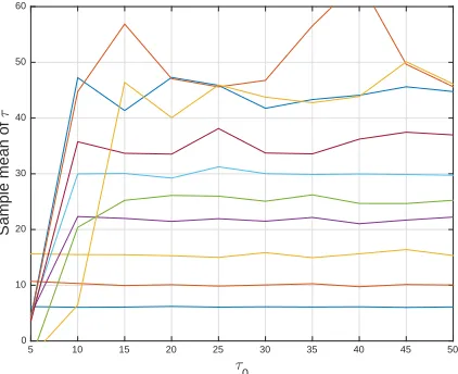
In Figure 2 we look at the recovery of the true value of τ with the hierarchical method. For large enough τ0, the mean ofτ after the burn-in period is roughly
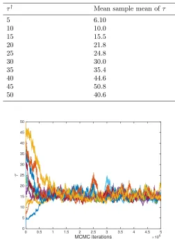
constant with respect to varying the initialization point, for each posterior. This makes sense from a theoretical point of view since these means arise from the same posterior distribution, for a fixed truth, but it is also reassuring from a computa-tional point of view since the output is close to independent of the initial guess for the length scale. There does however appear to be an issue with initializing the value of τ at too low a value, with the value τ tending to get stuck far from the truth when initialized at = 5. This effect has been detected in several other experiments and models – initializing the value of τ much lower than the true in-verse length can cause the parameter to become stuck in a local minimum. Such an effect has not been observed however when the parameter is initialized significantly larger than the true value. Table 1 shows that recovery of the true value of τ is very good forτ† ≤35, though becomes slightly worse for larger values ofτ†. The means here are calculated without theτ0= 5 sample means since they are clearly
in the casesτ† = 40, 45 and 50 is to do with the structure of the observation map
S. The observation grid has a length scale associated with it, related to distances between observation points, and so issues could arise when trying to detect the length scale of the geometric field that is significantly shorter than this. Addition-ally, the length scales 1/τ are closer for largerτ and so it may be more difficult to distinguish between particular values.
For brevity we now focus on the case where τ† = 15. The traces of the values ofτ along the hierarchical chains corresponding to this truth is shown in Figure 3. After approximately 106samples, all chains have become centered around the true
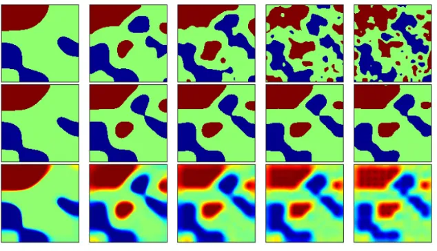
length scale. This convergence appears to be roughly linear for each chain. Figure 4 shows the push forwards of the sample means from the different chains under the level set map, that is, approximations ofF(E(u),E(τ)). This figure also
shows approximations ofE(F(u, τ)) and typical samples ofF(u, τ) coming from the
different chains. We see that these conditional means for the hierarchical method appear to agree with one other. This is reassuring for the reason mentioned above – they are all estimates of the mean of the same distribution. The figures for the non-hierarchical posteriors admit greater variation, especially near the boundary for higher values of τ. Moreover, not all inclusions are detected when the length scale parameter is taken to be τ = 5. Note that the mean from the hierarchical posterior agrees closely with that from the non-hierarchical posterior using the fixed true length-scaleτ= 15. Additionally, even though the means are reasonable approximations to the truth in most cases, the typical samples are much worse when using the non-hierarchical method with an incorrect length scale parameter. We can also consider the sample variance of the pushforward of the samples by the level set map, i.e. approximations of the quantity Var(F(u, τ)). In Figure 5 we show this quantity for both the hierarchical and non-hierarchical priors. Note that for the non-hierarchical priors, the variance increases both at the boundary and away from the observation points for larger values ofτ. Variance is also higher along the interfaces and within the central phase, since points in these locations are more likely to switch between all three phases. The hierarchical approximations all appear to agree. Whilst the hierarchical means are very similar to the non-hierarchical means using the true length scale, as seen in Figure 4, the non-hierarchical variances are smaller away from the observation points.
Additionally, we look at the level set function u itself in Figure 6. In these plots we rescale the level set function by τα−d/2 = τ4 so that they are all of
approximately the same amplitude. The means for both the hierarchical and non-hierarchical methods are again quite similar to one another, though the difference between the typical samples is much more stark.
Finally, in Figure 7, we look at the joint densities of the inverse length scale parameterτ and first five Karhunen-Lo`eve (KL) modes of the level set functionu.4 Non-trivial correlations are evident between τ and each of these modes, with the support of the densities appearing convex. This is likely related to the non-linear scaling between the length-scale and the amplitude of the level-set function under the prior. Conversely the KL modes, whilst still correlated with one-another other, have simpler joint densities. Note, also, that the posterior on the length scale is centered close to the true value of the inverse length scale parameterτ.
4KL modes are the eigenfunctions of the covariance operator, here ordered by decreasing
τ 0
5 10 15 20 25 30 35 40 45 50
Sample mean of
τ
[image:18.612.199.410.129.301.2]0 10 20 30 40 50 60
Figure 2. (Identity model) The sample mean ofτalong each
hier-archical MCMC chain, against the initial value ofτ. The different curves arise from using different datayi.
Remark 4.1. In this section we studied the ability to recover the true length scale parameter τ†, given a finite number of direct noisy observations of the geometric field. The question arises of how the quality of this recovery depends upon the spatial resolution of the data. As would be expected, learning this parameter becomes more difficult when this resolution is poor due to the lack of information in the data. However it is interesting to note that, even in the limit of an infinite number of distinct observation points, it is unlikely that we would be able to identify τ†
perfectly. This is suggested by a result of Zhang [57] which states that, in the context of generalized linear mixed models, the marginal variance and length-scale parameters of a Mat´ern field cannot be consistently estimated in this limit where as in our case the domain is fixed. This is in contrast to the case of additional data points increasing the domain, where consistent estimation is possible [32].
4.3. Identification of Geologic Facies in Groundwater Flow. The identifica-tion of geologic facies in subsurface flow applicaidentifica-tions is a common example of a large scale inverse problem that involves the recovery of unknown interfaces. In the case of groundwater flow, for example, the inverse problem concerns the recovery of the interface between regions with different hydraulic conductivity given measurements of hydraulic head. Geometric inverse problems of this type have recently received a lot of attention by the research community [39, 40, 44, 56]. Indeed, it has been recognized that the geometry determined by the aforementioned interfaces consti-tutes one of the main sources of uncertainty that must be quantified and reduced by means of Bayesian inversion.
Table 1. (Identity model) The value ofτ used to create the data yi, and the mean value of τ across the MCMC chains and the different initial values ofτ.
τ† Mean sample mean ofτ
5 6.10
10 10.0
15 15.5
20 21.8
25 24.8
30 30.0
35 35.4
40 44.6
45 50.8
50 40.6
MCMC iterations ×106
0 0.5 1 1.5 2 2.5 3 3.5 4 4.5 5
τ
0 5 10 15 20 25 30 35 40 45 50
Figure 3. (Identity model) The trace ofτalong the MCMC chain,
when initialized at the 10 different initial values. True inverse length scale isτ = 15.
(a)The true geometric field used to generate the datay, with true inverse length scaleτ= 15
(b)(Top) Representative samples of F(u, τ) under the hierarchical posterior. (Middle) Approximations ofF(E(u),E(τ)). (Bottom)
Ap-proximations of E(F(u, τ)). From left-to-right, τ is initialized at
τ= 5,15,25,35,45.
[image:20.612.149.466.494.676.2](c)As in (b), using the non-hierarchical method. From left-to-right, τis fixed atτ= 5,15,25,35,45.
Figure 5. (Identity model) Approximations of Var(F(u, τ)) using the hierarchical (top) and fixed (bottom) priors, initialized or fixed atτ= 5,15,25,35,45, from left-to-right. True inverse length scale isτ= 15.
Figure 6. (Identity model) Representative samples τ4·u (top) and sample means E(τ4 ·u) (bottom) of the level set function.
The rescaling τ4 means that the above quantities have the same approximate amplitude. True inverse length scale isτ= 15. (Left) Using the non-hierarchical method; from left-to-right τ is fixed at τ = 5,15,25,35,45. (Right) Corresponding quantities for the hierarchical method.
4.3.1. The forward model. We are interested in the identification of a piecewise constant hydraulic conductivity, denoted byκ, of a two-dimensional confined aquifer whose physical domain is D = [0,6]×[0,6]. We assume single-phase steady-state Darcy flow. The piezometric head, denoted byh(x) (x∈D), which describes the flow within the aquifer can be modeled by the solution of [6]
− ∇ ·κ∇h =f inD
(12)
wheref represents sources/sinks and where boundary conditions need to be spec-ified. For the present work we consider the setup from the Benchmark used in [14, 27–31]. In concrete, we assume thatf is a recharge term of the form
f(x1, x2) =
0 if 0< x2≤4,
137 if 4< x2<5,
274 if 5≤x2<6.
[image:21.612.129.514.317.428.2]Figure 7. (Identity model) (diagonal) Empirical densities of τ
and the first five KL modes of u. (off-diagonal) Empirical joint densities. True inverse length scale isτ= 15.
and we consider the following boundary conditions
(14)
h(x1,0) = 100,
∂h ∂x1
(6, x2) = 0,
−κ∂h ∂x1
(0, x2) = 500,
∂h ∂x2
(x1,6) = 0.
We consider the inverse problem of recoveringκfrom observations{`j(h)}64
j=1of hgiven by (12)-(14). We assume we have smoothed point observations given by
`j(h) =
Z
D 1 2πε2e
− 1
2ε2(x−qj)2h(x) dx
whereε >0 and{qj}64j=1⊆D is a grid of 64 observation points equally distributed
onD. Let Z =Lp(D) for some 1 ≤p <∞ andY =
given by (12)-(14). Then the forward mapS:Z→Y is given by
κ7→(`1(h), . . . , `64(h)).
We assume that eachκi in the definition of the level set mapF is strictly positive. The image ofF is contained in the set of bounded fields on D bounded below by miniκi >0. In [31] the mapS is shown to be continuous and uniformly bounded on such fields, with respect tok · kLp(D)for somep, and so Assumptions 1 hold. As
a consequence Theorem 2.4 applies directly.
4.3.2. Simulations and results. In the previous example we illustrate, with a simple model, the capabilities of the proposed framework to recover a specified true length-scale and a true level set function that defines a true discontinuous field from which synthetic data are generated. However, we must reiterate that, in practice, we wish to recover the true discontinuous field; the level set function is merely an artifact that we use for the parameterization of such a field. In practical applications the aim of the proposed hierarchical Bayesian level set framework is to infer a length-scale alongside with a level set function which, by means of expression (7), produces a discontinuous field that captures the desired piecewise constant field as accurately as possible and, in particular, the intrinsic length-scale separation of the interfaces determined by the discontinuities of the true geometric field. Therefore, in order to test our methodology in the applied setting of groundwater flow, rather than a true level set function, in this subsection we consider the true hydraulic conductivityκ†whose logarithm is displayed in Figure 9(a). Thisκ† is defined such that it takes the constant valuese1.5,e4 ande6.5. This is channelized conductivity
typical of fluvial environments and often used as Benchmarks for subsurface flow inversion [31, 40, 44, 56]. Note that the values that the conductivity can take on the three different regions differ by at least one order of magnitude, due to the logarithmic transformation. While there is indeed an intrinsic length-scale in the channelized structure, this true conductivity field does not come from a specified level set prior.
Synthetic data are generated by means of
y= (`1(h†), . . . , `64(h†)) +η, η∼N(0,Γ) i.i.d.
where h† is the solution to (12)-(14) for κ = κ†. Equations (12)-(14) have been solved with cell-centered finite differences [5]. In order to avoid inverse crimes, synthetic data are generated on a grid finer (160×160 cells) than the one used for the inversion (80×80 cells). The discretization is performed via the DFT, and we retain all modes. In addition, Γ is a diagonal matrix given by Γi,i= 0.0175`i(h†). In other words, we add noise that corresponds to 1.75% of the size of the noise-free observations. On the prior for the level set functionuwe take Neumann boundary conditions and fix the smoothness parameterα= 5.
We consider a Gaussian priorN(35,102) forτ, and use a Gaussian random walk
proposal distribution for this parameter. We then apply the hierarchical MCMC method from subsection 3.3 initialized with the following six different choices of
18. In the top row of Figure 9(b) we display the logarithm of some representatives samples of F(u, τ) under the hierarchical posterior. The middle row of Figure 9(b) shows the logarithm of F(E(u),E(τ)), i.e., the pushforward of the posterior
means obtained using the hierarchical method. The bottom row of Figure 9(b) displays the logarithm of the approximations of E(F(u, τ)). That is, the expected value of the pushforward samples under the posterior. The aforementioned results corresponds to five MCMC chains withτinitializedτ = 10,30,50,70,90 (the results forτ= 1 have been omitted). Similarly, Figure 10 (top) shows the approximations of the variance of the pushforward samples of the posterior, i.e. Var F(u, τ)
. Clearly, bothE(F(u, τ)) andF(E(u),E(τ)) result in fields that provide a reasonable
approximation of the true geometric field. Note that, as expected, the largest uncertainty in the distribution of the pushforward samples is around the interface between the regions with different conductivity. In Figure 11(a) we show some representative samples of u(top) and approximations toE(u) (bottom). In these
plots, as before, we rescale the level set function by τα−d/2=τ4 so that they are
all of approximately the same amplitude. In Figure 12 we display the empirical densities ofτ and the first five KL modes ofu. A key observation is that, although the true hydraulic conductivity is not generated by thresholding a Gaussian random field, and hence there is no “true” length scale, the posterior nonetheless settles on a narrow range of values ofτ which are consistent with the data.
From the aforementioned results we can also clearly see that the hierarchical MCMC algorithm produces similar outcomes regardless of the initialization of the inverse of the length-scaleτ, reflecting ergodicity of the Markov chain. The results fromτ = 1 are not shown but they are very similar to the ones from other chains. As with the results from the previous subsection, the similarity in outcomes be-tween all six chains is not surprising as these are aimed at sampling from the same posterior distribution; but the fact that this posterior distribution onτconcentrates near to a single value is of particular interest because it shows that the true geomet-ric field has an intrinsic length-scale, even though it was not constructed via the map F(u, τ). Furthermore, this similarity of outcomes between chains showcases the main advantage of the proposed framework with respect to the non-hierarchical one. Indeed, as stated earlier, the proposed method has the ability to recover a distribution for the intrinsic length-scale which gives rise to reasonably accurate estimates (i.e. F(E(u),E(τ)) andE(F(u, τ))) of the true geometric field. We now
present the numerical results from applying a non-hierarchical MCMC algorithm in which the inverse of length-scaleτ is fixed. We consider again six MCMC chains as before with the (now fixed) values ofτ= 1,10,30,50,70,90 that we used to initial-ized the hierarchical chains used before. Analogous results to the ones presented for the hierarchical method can be found in the bottom panels of Figure 9 as well as the bottom of Figures 10 and 11. Clearly, the lack of properly prescribing the intrinsic length-scale in the non-hierarchical method results in inaccurate estimates of the true geometric field. We clearly observe that forτ ≥30 the estimates of the truth given by F(E(u),E(τ)) and E(F(u, τ)) are substantially inaccurate and the uncertainty measured by Var F(u, τ)
is large. The non-hierarchical MCMC for
Figure 8. (Groundwater flow model) Trace plots of τ obtained
from six hierarchical MCMC chains.
4.4. Electrical Impedance Tomography. Finally we consider the electrical impedance tomography (EIT) problem. This problem has previously been ap-proached with a non-hierarchical Bayesian level set method [20]. In this subsection we show that the hierarchical approach outperforms the non-hierarchical approach in the case where the true conductivity is a binary field, given the same number of forward model evaluations.
4.4.1. The forward model. EIT is an imaging technique which attempts to infer the internal conductivity of a body from boundary voltage measurements. Typical applications include medical imaging, as well as subsurface imaging where it is known as electrical resistivity tomography (ERT). We utilize the complete electrode model (CEM), proposed in [49]. This is a physically accurate model which has been shown to agree with experimental data up to measurement precision. The strong form of the PDE governing the model is given by
−∇ ·(κ(x)∇v(x)) = 0 x∈D
Z
el
κ∂v
∂ndS=Il l= 1, . . . , L
κ(x)∂v
∂n(x) = 0 x∈∂D\ SL
l=1el
v(x) +zlκ(x)
∂v
∂n(x) =Vl x∈el, l= 1, . . . , L.
HereD⊆R2is the domain and{el}Ll=1⊆∂Dare electrodes on the boundary upon
0 1 2 3 4 5 6 0
1 2 3 4 5 6
1.5 2 2.5 3 3.5 4 4.5 5 5.5 6 6.5
(a)(Left) Logarithm of the true hydraulic conductivity field used to generate the data y. (Right) True pressure field, and the grid of observation points.
(b)(Top) Logarithm of representative samples ofF(u, τ) under the hierarchical posterior. (Middle) Logarithm of the approximations of F(E(u),E(τ)). (Bottom) Logarithm of the approximations of
E(F(u, τ)). From left-to-right,τis initialized atτ= 10,30,50,70,90.
[image:26.612.152.462.478.652.2](c)As in (b), using the non-hierarchical method. From left-to-right, τis fixed atτ= 10,30,50,70,90.
Figure 10. (Groundwater flow model) Approximations of Var F(u, τ)
using the hierarchical (top) and the non-hierarchical (bottom) MCMC.
(a)(Top) Representative samples of the rescaled level-set function τ4·uand (bottom) approximations of
E(τ4·u) using the hierarchical
method. From left-to-right,τis initialized atτ= 10,30,50,70,90.
[image:27.612.149.467.482.595.2](b)As in (a), using the non-hierarchical method. From left-to-right, τis fixed atτ= 10,30,50,70,90.
Figure 11. (Groundwater flow model) Representative samples
and sample means of the level set function. The rescalingτ4means
Figure 12. (Groundwater flow model) (diagonal) Empirical den-sities ofτand the first five KL modes ofu. (off-diagonal) Empirical joint densities.
the conductivity of the body and v represents the potential within the body5. It should be noted that the solution of this PDE comprises both a potentialv∈H1(D) and a vector{Vl}Ll=1 of boundary voltage measurements.
The inverse problem we consider is the recovery ofκfrom a sequence of boundary voltage measurements. A number of (linearly independent) current stimulation patterns {Il}Ll=1 may be performed to provide more information; we assume that
we perform the maximum M = L−1 measurements. Let Z = Lp(D) for some 1≤p <∞andY =RJ whereJ =LM. We can concatenate the boundary voltage measurements arising from different stimulation patterns to yield a mapS:Z →Y,
5In the EIT literature the conductivity field is often denotedσ, however we have already used this
κ7→(V(1), V(2), . . . , V(M)) whereV(m)={V(m)
l } L l=1∈R
L,m= 1, . . . , M.
For the experiments we work on a circular domain D={x∈R2 | |x|<1}. 16
electrodes are spaced equally around the boundary providing 50% coverage. All contact impedances are taken to bezl = 0.01. Adjacent electrodes are stimulated with a current of 0.1, so that the matrix of stimulation patterns I ={I(j)}15
j=1 ∈ R16×15 is given by
I= 0.1×
+1 0 · · · 0
−1 +1 · · · 0
0 −1 . .. 0 ..
. ... . .. +1
0 0 0 −1
.
We define our forward map G : X ×R+ →
RJ by G = S ◦ F. As in the
groundwater flow example, assume that each κi in the definition of the level set map is strictly positive. We do not have a continuity result for the map S on
Lp for any 1 ≤ p < ∞. However the almost-sure continuity of the map G can be seen via a modification of the proof of Proposition 3.5 in [20] to include the parameterτ; this modification is almost identical to the proof of Proposition A.1 given in the appendix. The uniform boundedness ofG follows from a result in [20] similarly. Hence as was the case with the identity map example, the conclusions of Proposition A.1 follow, and we can deduce the conclusions of Theorem 2.4.
4.4.2. Simulations and results. We fix a true conductivityκ†, shown in Figure 14. As with the groundwater flow experiments, this is constructed explicitly and does not have a true value ofτ associated with it. We generate datay as
y=S(κ†) +η, η ∼N(0,Γ)
where we take the noise covariance Γ = 0.00022·I to be white. The mean relative error on the generated data is approximately 12%. The data is generated using a mesh of 43264 elements and simulations are performed used a mesh of 10816 elements, in order to avoid an inverse crime. Forward solves are performed using the EIDORS software [1]. All level set field samples are defined on the square [−1,1]2 and restricted to the domain D. This has the advantage of allowing for
efficient sampling via the Fast Fourier Transform, though has the drawback of introducing possibly non-trivial boundary effects on the domain; no such effects are observed in our problem, however. The discretization on the square is performed via the DFT on a grid of 27×27 points, and we retain all modes.
The level set mapF is defined such that there are 2 phases, taking the constant values 1 and 10. We take the prior level set field mean to be zero, so that in this case
F (and hence Φ) becomes independent ofτ. Thus a forward model evaluation is not required for the Gibbs update ofτ, and each sample of (u, τ) using the hierarchical method costs virtually the same as one ofuusing the non-hierarchical method.
and again use Neumann boundary conditions. We again wish to compare how the hierarchical method compares with the non-hierarchical method. We therefore also look at the 5 different posterior distributions that arise when using each of 5 fixed prior inverse length scalesτ= 10,30,50,70,90, which gives another 5 MCMC chains. For both the methods we produce 4×10⁶ samples for each chain, and
discard the first 2×10⁶ samples as burn-in when calculating quantities of interest.
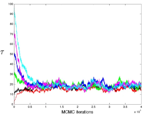
The traces of the values ofτ along the hierarchical chains are shown in Figure 13. With the exception of the chain initialized at τ = 10, the chains converge to the sample approximate value ofτ. Unlike in previous experiments, the traces have a relatively flat period before the approximate linear convergence to the common length scale. Initializing τ = 90 requires an additional 106 samples to converge,
over the other converging chains.
Figure 14 shows the push forwards of the sample means from different chains un-der the level set map, along with approximations ofE(F(u, τ)) and typical samples
ofF(u, τ) coming from the different posteriors. In both the hierarchical and non-hierarchical methods, the chains initialized/fixed atτ = 10 fail to recover the true conductivity, similarly to what was observed with the identity map experiments when initializing at τ = 5. The other chains for the hierarchical method produce very similar results to one another, whilst the effect of fixing the length scale to be too short is apparent in the figures for the non-hierarchical method.
In Figure 15 we see approximations to Var(F(u, τ)) under the different posteriors. In both cases, variance is highest around the boundaries of the two inclusions. The difference between the hierarchical and non-hierarchical methods is more apparent here, with higher variance between the two inclusions when the length scale is fixed to be too short.
Again, we look at the level set function u itself in Figure 16. In these plots, as before, we rescale the level set function by τα−d/2 = τ4 so that they are all
of approximately the same amplitude. As in the previous experiments, there is noticeable contrast between the means for the hierarchical and non-hierarchical methods, and yet more contrast between the typical samples.
Finally, in Figure 17, we show the posterior densities on the inverse length scale and the first five KL modes, as well as correlations between them. As with the groundwater flow example, although there is no “true” inverse length scale, the data is sufficiently informative to define a small range of values for this parameter under the posterior.
5. Conclusions
The level set method is an attractive approach to inverse problems for the de-tection of interfaces. Furthermore the Bayesian approach is particularly desirable when there is a need to quantify uncertainty. In this paper we have shown that Bayesian level set inversion is considerably enhanced by a hierarchical approach in which the length scale of the underlying level set function is inferred from the data. We have demonstrated this by means of three examples of interest arising in, respectively, the information, physical and medical sciences; however many poten-tial applications remain to be explored and this provides an interesting avenue for future work.
MCMC iterations ×106
0 0.5 1 1.5 2 2.5 3 3.5 4
τ
[image:31.612.196.409.127.299.2]0 10 20 30 40 50 60 70 80 90
Figure 13. (EIT model) The trace ofτ along the MCMC chain,
when initialized at the 5 different valuesτ= 10,30,50,70,90.
updating the level set function and the length-scale. The Metropolis method we use for the level set field update does not use derivatives of the log-likelihood, and could be improved by doing so, using the infinite dimensional variants on MALA and HMC (which use first derivative information, see the citations in [16]) or the manifold MALA and HMC methods, which use higher order derivatives [25]. Another interesting direction for future work is the design of methods with more informed proposals which exploit correlations in the level set function and its length-scale. And finally it would be interesting to consider pseudo-marginal methods to sample the hierarchical parameter alone, as in [21].
Assuming independence under the prior, it would require little further work to treat the thresholding levels {ci} and the values of the thresholded function{κi} as part of the inference as well; we omitted this here for the sake of clarity. Such a model may be more realistic, and numerical studies of such models may prove interesting. Another extension of interest may be to place a hyperprior upon the regularity parameter also, which may be useful for improving rates of convergence [54]. This is a more challenging task, again related to singularity of measures. The paper [2] discusses ways in which this may be done, however it is still an open question in terms of theory and optimal algorithms. Additionally, it may be of interest to overcome the restriction of the ordering of phases {κi} by means of a vector level set method [52].
Finally we mention that the use of a single length-scale within an isotropic prior is a simple example of more sophisticated hierarchical approaches which attempt to learn non-stationary and non-isotropic [12, 13] features of the level set function from the data. This provides an interesting opportunity for future work and for ideas from machine learning to play a role in the solution of inverse problems for interfaces.
1
10
j
0 50 100 150 200 250
yj
-0.06 -0.04 -0.02 0 0.02 0.04 0.06
(a)(Left) True conductivity field used to generate the datay. (Right) The entriesyiof
the data vectory, plotted againsti.
(b)(Top) Representative samples of F(u, τ) under the hierarchical posterior. (Middle) Approximations ofF(E(u),E(τ)). (Bottom) Ap-proximations of E(F(u, τ)). From left-to-right, τ is initialized at τ= 10,30,50,70,90.
[image:32.612.213.407.122.196.2](c)As in (b), using the non-hierarchical method. From left-to-right, τis fixed atτ= 10,30,50,70,90.
20
[image:33.612.147.468.115.237.2]0 10
Figure 15. (EIT model) Approximations of Var(F(u, τ)) using
the hierarchical (top) and fixed (bottom) priors, withτ initialized or fixed atτ = 10,30,50,70,90, from left-to-right.
(a)(Top) Representative samples of the rescaled level-set function τ4·uand (bottom) approximations of
E(τ4·u) using the hierarchical
method. From left-to-right,τis initialized atτ= 10,30,50,70,90.
(b)As in (a), using the non-hierarchical method. From left-to-right, τis fixed atτ= 10,30,50,70,90.
Figure 16. (EIT model) Representative samples and sample
[image:33.612.152.469.302.421.2]