1
Using a rolling training approach to improve judgmental extrapolations
elicited from forecasters with technical knowledge
Fotios Petropoulos
1,*, Paul Goodwin
2and Robert Fildes
31Cardiff Business School, Cardiff University, UK 2
School of Management, University of Bath, UK 3
Lancaster Centre for Forecasting, Lancaster University, UK
* corresponding author: [email protected]
Abstract
Several biases and inefficiencies are commonly associated with the judgmental extrapolation of time
series even when forecasters have technical knowledge about forecasting. This study examines the
effectiveness of using a rolling training approach, based on feedback, to improve the accuracy of
forecasts elicited from people with such knowledge. In an experiment forecasters were asked to make
multiple judgmental extrapolations for a set of time series from different time origins. For each series
in turn, the participants were either unaided or they were provided with feedback. In the latter case,
following submission of each set of forecasts, the true outcomes and performance feedback were
provided. The objective was to provide a training scheme, enabling forecasters to better understand
the underlying pattern of the data by learning directly from their forecast errors. Analysis of the
results indicated that the rolling training approach is an effective method for enhancing judgmental
extrapolations elicited from people with technical knowledge, especially when bias feedback is
provided. As such it can be a valuable element in the design of software systems that are intended to
support expert knowledge elicitation (EKE) in forecasting.
Keywords: judgmental forecasting, unaided judgments, rolling training, feedback, time series, expert
2 1. Introduction
Surveys suggest that forecasts based either wholly or in part on expert management judgment play a major role in company decision making (e.g. Fildes and Goodwin, 2007). Sometimes the judgmental inputs may take the form of adjustments to statistical forecasts, ostensibly to take into account special factors that were not considered by the statistical forecast (Fildes, Goodwin, Lawrence, and Nikolopoulos, 2009). However, in some circumstances, judgment may be the only process involved in producing the forecasts. This may even be the case in situations where a statistical forecast is provided but the expert chooses to ignore it (Franses, 2014). In some cases judgment is used to extrapolate time series data to produce point forecasts, when no other information (except perhaps variable labels such as ‘sales’ or ‘costs’) is provided. This type of task has been the subject of much research over the last thirty years and a number of biases associated with judgmental extrapolation have been identified. These include tendencies to overweight the most recent observation (e.g. O’Connor, Remus, and Griggs, 1993), to underestimate growth and decay in series (Lawrence, Goodwin, O’Connor, and Onkal, 2006) and a propensity to see systematic patterns in the noise associated with series (Eggleton, 1982; O’Connor, Remus, and Griggs, 1993).
Such biases can apply even where the forecaster has expertise, either in the domain within which the forecasts are being made (e.g. Pollock and Wilkie, 1993) or has technical knowledge of forecasting (Goodwin and Fildes, 1999). This suggests that, when experts are called upon to make judgmental extrapolations, the elicitation process may benefit from the inclusion of devices designed to mitigate these biases. Studies in the expert knowledge and elicitation (EKE) literature have examined a number of ways of designing elicitation methods so that they reduce the danger of biased judgments from experts, particularly in relation to the estimation of probabilities or probability distributions (e.g., Aspinall, 2010, Morgan, 2014, Bolger and Rowe, 2014, Goodwin and Wright, 2014, Chapter 11). Our focus here is on improving EKE in time series extrapolation.
3
This paper reports on an experiment that was designed to explore the effectiveness of providing rolling feedback to forecasters on the outcomes of the variable they are attempting to predict and on their forecasting performance. The objective is to provide a direct training scheme, enabling forecasters, who already have technical knowledge, to better understand the underlying pattern of the
data by learning directly from their forecast errors and thereby improving the accuracy of the judgments elicited from them. Two types of performance feedback were compared: feedback on the bias associated with the submitted forecasts and feedback on their accuracy. The paper is structured as follows. A review of the relevant literature is followed by an outline of the research questions that were investigated. Details of the experiment and presentation of the analysis and results follow this. Finally, the practical implications of the findings are discussed and suggestions made for further work in this area.
2. Literature review & research questions
In judgmental forecasting Sanders and Ritzman (1992) distinguish between expertise that is founded on contextual knowledge and that which is based on technical knowledge. Expertise relating to contextual knowledge results from factors such as experience of working in an industry and possessing specific product knowledge. In contrast, expertise based on technical knowledge is present when a forecaster has knowledge about formal forecasting procedures, including information on how to analyze data judgmentally.
Sanders and Ritzman compared the forecasting accuracy of: i) managers who had contextual expertise but lacked technical expertise, ii) forecasters who lacked contextual expertise but had technical expertise iii) forecasters who lacked both contextual and technical expertise. They concluded that expertise based on technical knowledge had little value in improving the accuracy of judgmental forecasts when compared with expertise based on contextual knowledge. However, many of the time series they studied were highly volatile and contextual factors, rather than time series components, accounted for much of their variation. The forecasters with technical expertise who took part in the study were not privy to these contextual factors.
4
with technical knowledge had a lower average median absolute percentage error (MdAPE) than those without this knowledge in 13 out of 17 series (p=0.025 on a binomial test of the hypothesis that each group had an equal probability of achieving the lowest MdAPE on a given series). Although the mean reduction in these average MdAPEs was only 1.8% for the 17 series the results provide some evidence that, when extreme volatility is not present in series, there may, after all, be advantages in eliciting forecasts from people possessing technical expertise. This also raises the possibility that these judgments may be enhanced through further training.
In a review of the Sanders and Ritzman (1992) study Collopy (1994) argues that people may not always be able to apply what they learn in a training process. He cites a report by Culotta (1992) who found that even students who do well in calculus courses cannot apply what they learned. Those with technical knowledge in the Sanders and Ritzman study had taken an elective course in forecasting and may therefore have been subject to didactic learning which is a relatively passive process. This is contrasted with experiential learning which includes actively participating in the task for which one is being trained, reflecting on the experience and learning from feedback (Moon, 2004). Training of this type may therefore be effective in obtaining improvements in accuracy by those with technical expertise.
For experiential training to be effective it will need to address the specific challenges of the task (Kremer et al., 2011). Goodwin and Wright (1993, 1994) argue that three components of a time series influence the degree of difficulty associated with the judgmental time series forecasting task. These
are: (1) the complexity of the underlying signal, comprising factors such as its seasonality, cycles and trends and autocorrelation; (2) the level of noise around the signal; and (3) the stability of the underlying signal.
5
Several studies have suggested that judgmental forecasters often confuse the noise in the time series with the signal (Andreassen, 1998; Harvey, 1995; Lopes and Oden, 1987, Reimers & Harvey, 2011). For example, they often adjust statistical forecasts to take into account recent random movements in series which they perceive to be systematic changes that were undetected by the statistical forecast (Goodwin and Fildes, 1999). Conversely, when systematic changes in the signal do occur, forecasters may delay their response to this, perceiving the change to be noise (O’Connor et al., 1993). Also, they may pay too much attention to the latest observation, which will contain an element of noise (Bolger and Harvey, 1993; Lawrence and O’Connor, 1992). It seems reasonable to expect that noise can also impair the detection of underlying trends and seasonal patterns, though this was not the case in two studies where series were presented graphically (Lawrence and Makridakis, 1989; Mosteller, Siegel, Trapido and Youtz, 1981).
Learning through feedback can potentially mitigate these biases (Lawrence et al. 2006). As we indicated above feedback is a key component of experiential learning. Feedback has been shown to improve the accuracy of point forecasts (Goodwin and Fildes, 1999; Remus, O’Connor and Griggs, 1996; Sanders, 1997; Welch, Bretschneider and Rohrbaugh, 1998). However, there are a number of different types of feedback that may be particularly relevant to the time series forecasting task (Balzer, Doherty and O’Connor, 1989; Onkal and Muradoglu, 1995) and more research is needed to determine the most effective type and how it should be delivered.
6
moving averages of performance may help to solve the dilemma, but they may be less transparent and understandable to the recipients of the feedback. Another option would be simply to supply a set of point errors for n recent periods without using any kind of average. This could potentially enable the forecaster to identify specific problematic periods that invite attention (for example seasonality peaks). Moreover, in a rolling origin scheme, this strategy provides a way to check if point errors are reducing over time.
We might expect different types of performance feedback to vary in their effectiveness. Feedback on bias can provide a direct message that one’s forecasts are typically too high or too low and hence suggest how they might be improved. This is likely to be beneficial for untrended series or series with monotonic trends. However, it may lead to unwarranted confidence in one’s current forecasting strategy when series have alternating patterns or seasonal patterns because biases in different periods will tend to cancel each other out if an average across the signed errors is to be used. Feedback on accuracy, in contrast, provides no such direct message and its implications may be difficult to discern. If forecasters are to learn from accuracy feedback they will need to experiment with alternative approaches, not specified by the feedback, and then establish if these have led to improved accuracy. This will require comparisons of accuracy across different periods adding to the forecaster’s cognitive burden. Thus accuracy feedback seems unlikely to be conducive to rapid learning. This may explain the ineffectiveness of performance feedback in a study by Remus et al. (1996) which consisted only of an accuracy measure (the mean absolute percentage error).
Other forms of feedback seem likely to be less relevant to practical judgmental time series forecasting contexts. Cognitive process feedback aims to provide forecasters with insights into their own forecasting strategy, causing them to reflect on the possible deficiencies of this strategy (O’Connor, Remus and Lim, 2005). For example, a regression model may be used to attempt to capture their strategy so that the weights implicitly being attached to different items of available information, or cues, can be identified. In time series forecasting it will clearly take time to obtain sufficient information to estimate these weights reliably, thereby reducing the speed of learning by forecasters. Also, identifying the relevant cues to include in a model from the huge number of potential cues that are present in the time series forecasting task is problematical (e.g. typical cues might be the last observation, the mean of last n observations, the last difference between observations, the range of the last n observations and so on). In addition, many of these cues will be serially correlated so multicollinearity is likely to reduce the precision with which weights can be estimated.
7
forecasts. Task feedback has been widely researched elsewhere (e.g. Goodwin and Fildes, 1999; Sanders, 1997; Willemain, 1989; Willemain, 1991) and is not the topic of the current paper.
Ultimately, any form of feedback, regardless of its type, is likely to be most effective in enhancing judgments from those with technical expertise if it is easily and quickly understood (O’Connor et al,, 2005), and salient, accurate and timely (Lawrence et al., 2006). We therefore propose and test a rolling training scheme, based on performance feedback. This has a number of innovations that are designed to address the problems associated with feedback presented in earlier studies. Unlike these studies we have not supplied metrics that summarise ‘average’ performance over a number of periods or tasks (e.g., a mean absolute percentage error or a measure of calibration, which of necessity, has to be based on a summary of performance over large number of judgments). Instead, a performance measure is supplied for each individual judgment made by the forecaster so there is no arbitrary censoring of earlier performance and the balance between the sensitivity and stability of the feedback is no longer an issue. Furthermore, the feedback is ‘rolling’ so that a complete and growing record of the forecaster’s performance is presented and updated at regular intervals. These innovations are important because, as we have seen, a key problem with feedback based on ‘average’ metrics is that it can be dependent on the number of periods which contribute to the average. Also, when a time series contains cyclical or seasonal patterns, a tendency to forecast too low when the time series rises and too high when it falls will be masked by an ‘average’ metric. In the scheme proposed here, forecasters can link their errors to individual observations and patterns. They can also easily see if their performance is improving over time without having to memorise the previous value of the metric.
3. Experimental design
3.1. Forecasting approaches
Two judgmental forecasting approaches were evaluated in the current research. Each subject provided judgmental estimates with both approaches, using a fully symmetric experiment as we will discuss in sub-section 3.3.
Unaided Judgment: This is the simplest judgmental forecasting approach, while being quite popular. Humans are requested to provide their point forecasts all at once for all lead times (h), without receiving any kind of guidance, other than the past data points. This approach will act as the benchmark in our study and, hereafter, is referred to as UJ.
8
each are withheld (N > kh). At the first stage, only the first N - kh periods are presented to the forecaster, while h forecasts ahead are requested. Upon submission of the participants’ forecasts, the actual values of these h observations are presented, along with performance feedback in terms of percentage errors for each period (signed or not). This procedure is repeated for k times, with h data points being added in each repetition. Hence the completion of each training loop is followed by the submission of the h estimates for the future, unknown, periods. As such we, therefore, perform h -steps-ahead rolling evaluation (Tashman, 2000), which is common practice in automatic forecast model selection (Fildes and Petropoulos, 2015). In other words, this is a rolling origin (as opposed to a rolling observation window) forecasting procedure with updating every h periods, where the observation window is not kept constant but increases with the sample size. However, in this case, instead of selecting the best model based on out-of-sample performance, we assume that this procedure will assist the participants to better understand the time series patterns, thus providing more accurate forecasts. Hereafter, this approach is referred to as RT.
3.2. Time series
Most relevant studies that have focused on the impact of feedback for judgmental forecasting tasks made use of simulated series (e.g. Fischer and Harvey, 1999; Bolger and Onkal-Atay, 2004). Moreover, many studies did not examine seasonal series, confining their attention to stationary and trended ones (Bolger and Onkal-Atay, 2004; Lurie and Swaminathan, 2009). Therefore, in the current research we focus on real time series that collectively demonstrate a variety of characteristics (stationary, only trended, only seasonal and both trended & seasonal). More specifically, 16 quarterly series were manually selected from the M3-Competition data set (Makridakis and Hibon, 2000) so as to have the required characteristics. These were confirmed by autocorrelation function plots, Cox-Stuart/Friedman tests or by fitting an appropriate exponential smoothing model, using all the data. In addition, half of the trended and the seasonal series did not exhibit any significant pattern (trend or seasonality respectively) in the first two years, but did so later on. This selection was made in order to examine participants' adaption and ability to recognise developing series characteristics.
9
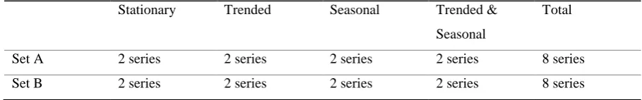
Table 1. Sets of series
Stationary Trended Seasonal Trended &
Seasonal
Total
Set A 2 series 2 series 2 series 2 series 8 series
Set B 2 series 2 series 2 series 2 series 8 series
The required length of all series was set to N=28 points (7 years), with longer series being truncated. In both UJ and RT approaches, the last 4 observations (last year) were withheld and used only for the out-of-sample evaluation and comparison of the two approaches. The length of this sample matches the required forecasting horizon, thus h=4. In addition, 12 observations were used for the RT procedure, thus, the number of blocks, k=3. The forecasting performance was tested on the last 4 observations (last year), where forecasts for both approaches (UJ and RT) were produced.
3.3. Participants & web application
The group of participants consisted of 105 undergraduate students enrolled in the Forecasting Techniques module of the School of Electrical & Computer Engineering at the National Technical University of Athens. During the module the students had been taught principles of time series analysis, statistical and judgmental forecasting methods, and how to evaluate forecasting performance. The experiment was introduced as an elective exercise, giving bonus credit for the 50% of the participants who produced the more accurate forecasts.
The group of 105 participants wwas eq
In order to attract a large number of participants, we decided not to perform a standard laboratory experiment, but to build a web application. The web application was specifically designed for the purpose of this experiment, using the ASP .NET framework for the web development of the front-end and a Microsoft SQL database for storing the time series data and participants’ point forecasts. The Microsoft Chart Controls library was used for drawing line and bar graphs as discussed in the next subsection. The application was hosted in a secure web-server where participants could connect remotely through their internet-enabled personal computers via any web browser.
3.4. Process of the experiment
10
using the UJ approach for 8 time series and then, at the next step, to submit their estimates under the RT approach for the remaining 8 series, while the opposite (first RT then UJ) was the case for the other half of the participants. Following this symmetric design allowed us to avoid any familiarity with the task effects that could have been arisen if the two approaches were always presented in the same order (first UJ then RT) for all the participants. When feedback was provided, each participant was randomly assigned to either the signed or unsigned percentage errors treatment (so that either bias or accuracy feedback was provided). Out of the 105 participants, 52 were given feedback on signed errors and 53 on absolute errors.
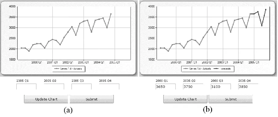
[image:10.595.73.524.471.662.2]All series were presented in a line graph format, using the color blue for the actual values and green for the submitted forecasts. While there is no evidence on the superiority of graphical or tabular numerical formats (Lawrence et al, 2006), a graphical representation is a more common feature in modern forecasting support systems. Historical data points were kept unlabeled in terms of the exact values, so that the participants could not export these values into a spreadsheet and use statistical approaches. This is a very important constraint, as the experiment took place in an unobserved environment and a graphical mode of presentation was the only way to guarantee that judgmental extrapolation is used. However, grid lines were provided in order to accommodate numerical estimations. Four text boxes were used for the input of judgmental forecasts for each lead time, while an update button could be used to refresh the graph, so that the subject could check his or her judgmental estimates graphically before submitting. Figure 1 presents two typical screens of the implemented system, before (a) and after (b) the input of the four point forecasts.
Figure 1. Screenshots of the system’s graphical representation and input features.
11
[image:11.595.148.450.232.471.2]Warming-up round: Each of the first four series was presented to the participants, withholding the last four observations. The participants were requested to provide judgmental point forecasts for the next four quarters (one year). A short description of each series was provided, describing any historical patterns. Upon submission of the forecasts for each series, forecast errors for each point (signed or not) were automatically calculated and displayed in bar charts, using the color red. As this round was a 'warm-up' the forecasts elicited were not taken into account when the results of the study were analysed. Figure 2 presents the screen with the information provided to the participants after the submission of the four point forecasts for a series.
Figure 2. Screenshot of the system’s feedback report features in terms of outcome (out-of-sample actual values)
and performance (error bars).
UJ round:The series from Set A (or Set B) were used, holding out the last four observations in each series. The series were presented in a random order. The participants were given the 24 actuals of each series in a graphical format and were requested to provide judgmental point forecasts for the next four quarters (periods 25 to 28). No description of the series and no information on the accuracy of the forecasts were provided.
12
third year set of forecasts was requested, again followed by outcome and performance feedback. Finally, the participants submitted their final four forecasts. In order to be directly comparable with the UJ, only the last set of forecasts were used in the evaluation. Moreover, when producing the final fourth year forecasts, the same amount of information (an observation window of 24 periods) was made available to participants as with the UJ approach.
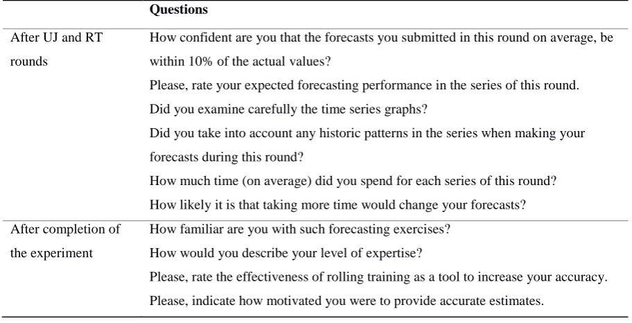
The completion of the latter two rounds was followed by a questionnaire which included questions on the participants’ confidence in the accuracy of their submitted forecasts, their expected forecasting performance, the extent to which they had examined the graphs and series patterns, and the time spent in producing their forecasts. In addition, a final questionnaire was used to ask participants about their familiarity with forecasting tasks, their level of forecasting expertise, their perceptions of the effectiveness of Rolling Training (RT) and their motivation to provide accurate estimates. The two sets of questions posed are displayed in Table 2. All questions were accompanied by 5-step ordinal response choices (Likert scale).
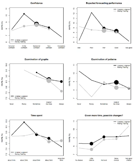
[image:12.595.70.526.442.675.2]The responses to the questions posed to the participants were analysed in order to examine any relationships between the variables in question (e.g., confidence, expected performance, extent of examination of graphs) to the actual forecasting performance achieved in the respective rounds of the experiment (UJ and RT). This analysis is presented and discussed in subsection 4.2.
Table 2. Questions posed to the participants Questions
After UJ and RT
rounds
How confident are you that the forecasts you submitted in this round on average, be
within 10% of the actual values?
Please, rate your expected forecasting performance in the series of this round. Did you examine carefully the time series graphs?
Did you take into account any historic patterns in the series when making your
forecasts during this round?
How much time (on average) did you spend for each series of this round?
How likely it is that taking more time would change your forecasts?
After completion of
the experiment
How familiar are you with such forecasting exercises?
How would you describe your level of expertise?
Please, rate the effectiveness of rolling training as a tool to increase your accuracy.
13 4. Analysis
4.1. Forecasting performance
Table 3 presents the percentage improvements in accuracy that were achieved by using RT when compared with UJ. These percentage improvements are measured as:
UJ s RT s MAE MAE median 1
100 (%)
where the UJ in the denominator is acting as the benchmark for this study. Negative values denote that RT performed worse than UJ. The median is calculated across the series considered in each case. In both the numerator and the denominator, the mean absolute error of a series s is calculated across the participants and horizons, as:
H h P p h p hs y f
P H MAE 1 1 , 1 1
where P denotes the number of participants, H the number of out-of-sample lead times, yh the actual
value of a series at time h and fp,h the forecast of participant p for the same series at time h. Note that
the number of participants (P) is not the same for all series, as a results of the slightly unequal sample sizes.
The results are analysed by columns in terms of series characteristics (stationary, trended, seasonal, trended & seasonal, low noise and high noise). Major rows indicate all (25th to 28th), near (25th to 26th)
or far horizons (27th to 28th). Minor rows provide additional analysis of the results based on the type of
14
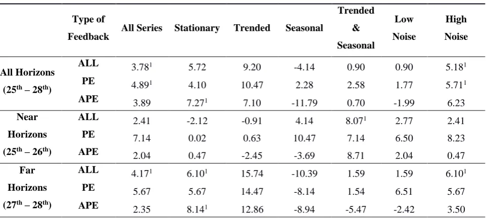
Table 3. Accuracy improvements (%) of RT approach over UJ
Type of
Feedback All Series Stationary Trended Seasonal
Trended & Seasonal Low Noise High Noise All Horizons (25th – 28th)
ALL 3.781 5.72 9.20 -4.14 0.90 0.90 5.181
PE 4.891 4.10 10.47 2.28 2.58 1.77 5.711
APE 3.89 7.271 7.10 -11.79 0.70 -1.99 6.23
Near Horizons (25th – 26th)
ALL 2.41 -2.12 -0.91 4.14 8.071 2.77 2.41
PE 7.14 0.02 0.63 10.47 7.14 6.50 8.23
APE 2.04 0.47 -2.45 -3.69 8.71 2.04 0.47 Far
Horizons (27th – 28th)
ALL 4.171 6.101 15.74 -10.39 1.59 1.59 6.101
PE 5.67 5.67 14.47 -8.14 1.54 6.51 5.67 APE 2.35 8.141 12.86 -8.94 -5.47 -2.42 3.50
1Differences are statistically significant at 0.05 level.
Overall, there is evidence that the RT approach results in statistically significant better forecasting performance (3.78% performance gain). Improvements are more prominent for high noise (5.18%, statistically significant at the 0.05 level). Although gains of 5.72% and 9.20% were observed for stationary and trended series, respectively, these were not statistically significant at the 0.05 level.
Focusing on the very first row of Table 3, where all horizons are considered, the only decrease in performance comes from the seasonal series. Even if this decrease is not statistically significant, suggesting that UJ and RT perform similarly, we attempt to understand the reason behind this result, by examining separately series with evident seasonality for the very first years or not, as discussed in section 3.2. This analysis suggested that RT might not suitable for series with developing seasonality. In terms of the type of feedback provided to the participants, it is apparent that bias feedback demonstrates the most significant improvements (4.89% overall), while improvements for accuracy feedback are generally smaller and not consistent. One could argue that providing errors in an absolute format may lead to confusion, as the participants may not be able to correctly evaluate this kind of information. On the other hand, bias feedback for each point in the form of signed bar charts is easier to interpret and understand and indicates a clear strategy for improving one’s forecasts. It is notable that bias feedback, which involved the provision of signed percentage errors for each individual period, improved accuracy for seasonal series. It is unlikely that providing a mean of these percentage errors would have been as effective because any tendency to over forecast for some seasons and under forecast for others would have been masked by the averaging process.
15
statistically significant at 0.05 level when all types of feedback are pooled together. However, the differences between RT and UJ for shorter horizon and low noise series are not statistically significant at the 0.05 level.. Lawrence, Edmundson and O’Connor (1985) suggested that, when the forecasting task is based on graphs, judgmental forecasts can be as good as statistical model forecasts at least for the shorter horizons. In contrast, longer horizons and series with high levels of noise constitute the cases where unaided judgmental forecasting is likely to be relatively inaccurate. The use of a direct rolling training scheme improves graph-based judgmental long-term forecasting, building on the efficiency of judgmental over statistical approaches.
4.2. Questionnaire responses analysis
16
Figure 3. Association between questionnaire responses and forecasting performance for the first set of questions
17
problem of judgemental forecasting, namely the underestimation of uncertainty (e.g. Makridakis, Hogarth and Gaba, 2009).
As expected, a propensity to examine graphs (and, to a lesser extent, patterns) has negative associations with the MAPE, suggesting that, as participants devote more time to this task, improvements in forecasting accuracy are recorded. However, literally no differences are observed between the two approaches (UJ and RT) in terms of mean values on the frequency in examining graphs and patterns. One would have expected that RT would better motivate the participants to examine the graphs and series patterns more carefully; however this was not the case.
The forecasting performance achieved with both UJ and RT is associated with the time the participants reported spending in producing the forecasts for each series – the more time they spent the greater the accuracy they achieved. However, the correlation is stronger in the case of UJ, meaning that forecasting performance achieved by the RT approach can be seen as more time invariant. Also, there is evidence that participants who were less accurate recognised that spending more time on the task might have resulted in changing their forecasts (this is particularly the case for the RT group).
The same analysis was performed for the second set of questions. The majority of the participants (76%) found the RT approach to be either effective or very effective. However, familiarity with forecasting exercises, perceived effectiveness of RT and motivation to produce accurate forecasts were only weakly or moderately associated with forecasting accuracy. Interestingly, the self-reported level of expertise of participants had a strong positive association with the realised MAPE so that those who considered themselves to have greater expertise produced less accurate forecasts. Further work would be needed to establish why this was the case but it is consistent with the Dunning-Kruger effect (Kruger and Dunning, 1999) where relatively unskilled people mistakenly consider that their ability is higher than it really is. Clearly, such an effect would have important implications for EKE if choices are made between experts’ forecasts based on their self-rated expertise.
5. Discussion & implications
18
discussed earlier, feedback on bias provides a clear indication of how future forecasts might be improved. In contrast, feedback on accuracy does not provide any indication of possible improvement strategies. Nor does it provide an indication of whether accuracy improvement is even possible. For example, does an APE of 10% represent the limit of the accuracy that can be achieved, given the noise level, or is there scope for further improvement?
Second, the attribute of the bias feedback that appeared to contribute to its effectiveness was the feedback of a set of individual errors, rather than an average of these errors. In series where the signal has autocorrelated elements such as seasonal series, judgmental biases may lead to positive errors at some stages of the cycle (e.g. where sales are increasing) and negative errors at other stages (e.g. where sales are decreasing). The presentation of individual errors allows each observed bias to be associated with individual periods and avoids the cancelling out of opposing biases that would be a feature of any averaging. Also, the need for appropriately selecting a length for averaging the point forecast errors is now removed.
Third, the presentation of the bias feedback as a bar chart may have enhanced its effectiveness, though further research would be needed to establish this. For example a set of four negative bars would be a strong, simple and clear indication that the previous set of forecasts was too high (error = actual –
forecast). A table of four numbers would probably provide a less salient message.
Fourth, the rolling nature of the feedback enabled it to reflect improvements in performance quickly, while at the same time avoiding the danger of confining attention to the performance of the most recent forecast (which is a danger of outcome feedback). Moreover, rolling across origins for one series, before moving on to the second one, helped the participants to focus on each series separately and better understand the improvements (or deterioration) in their performance over time. It is however an unrealistic representation of the typical forecasting task: more common is where feedback arises across time series.
Recent research suggests that the focus on enabling people to learn how to avoid bias is appropriate. A study by Sanders and Graman (2009) found that when translating forecast errors into costs (such as excessive inventory or labour costs) accuracy was less important than bias. In their survey of forecasters Fildes and Goodwin (2007) expressed surprise at the number of company forecasters who never checked the accuracy of their forecasts. The current study and the findings of Sanders and Graman (2009) suggest that monitoring and feeding back levels of bias may be just as, if not more, important than checking accuracy levels if the objective is to foster improved forecasts and minimize the costs of errors.
19
(lessons learned) from the achieved performance on the previous periods would probably be regarded as outdated. RT offers direct, timely and salient feedback on the performance over a number of periods focusing on a single series’ performance. The provision of the past forecast errors per period allows for the identification of specific periods where performance drops. These two features of RT enable forecasters to achieve better performance for the longer horizons and the most volatile series. This is due to the fact that RT essentially invites the forecasters to closely examine the series patterns across a number of horizons, rather than focusing only on the short-term forecasts. In addition, as the performance is provided in a rolling manner, forecasters are able to understand the limits of predictability for each series. As such, RT may have an important role to play, being particularly suitable for forecasting and decision making under low levels of predictability (i.e. where there is a high degree of uncertainty).
6. Conclusions & perspectives
Judgmental forecasting is widely employed in many contexts for estimating future values of time series. However, numerous studies have shown the limitations of judgment even when this is elicited from those with technical expertise. The current study examined the effectiveness of a rolling training scheme that provides direct feedback by reporting to participants their levels of performance in such a task. This involved reporting signed or absolute percentage errors for each period on a rolling basis, as opposed to metrics that summarise performance over several periods. Real time series featuring a number of characteristics were used. Participants provided estimates for both the control case (unaided judgment) and the test case (rolling training) leading to increased power. This was achieved by a symmetric experimental design. Although the analysis was not based on data collected in the field, the experimental approach allowed the effects of feedback of different types to be efficiently measured and compared under controlled conditions. Experiments like these have played a valuable role in areas such as behavioural operations management as one component of a process of triangulation with field research (Siemsen, 2011).
20
expertise acquired though didactic learning by providing experiential learning based on feedback that is accurate, timely, suggestive of how improvements might be made and easily interpreted.
One very interesting outcome is that improvements achieved by using a rolling training procedure are higher for longer forecasting horizons and noisy series. On top of the improvements achieved in forecasting performance, the rolling training procedure made the participants less confident in their forecasts. This is an additional advantage as there is evidence that people tend to under estimate the levels of uncertainty associated with their forecasts.
The current paper focused on analysing the performance over the final set of periods (the final year) contrasting unaided judgment with rolling training. However, a further objective of the current experimental design would be to analyse how the forecasting performance changes over time within a single series, as a direct result of the application of the rolling training procedure. Moreover, policy capturing regression models may provide insights of the forecasting strategy employed by participants with technical knowledge. This can include a large number of potential cues linked with time series forecasting. Of course, often the time series forecasting task is carried out in situations where contextual information (such as information from market research or information on advertising strategies) is available to expert forecasters in addition to time series data and it would be interesting to test the effectiveness of rolling training in this context.
References
Andreassen, P.B. (1988). Explaining the price volume relationship - the difference between price changes and changing prices. Organizational Behavior and Human Decision Processes, 41, 371-389. Annett, J. (1969). Feedback and Human Behaviour, Penguin Education.
Aspinall, W. (2010). A route to more tractable expert advice. Nature, 463(7279), 294-295.
Balzer, W.K., Doherty, M.E., & O'Connor, R. (1989). Effects of cognitive feedback on performance.
Psychological Bulletin, 106, 410-433.
Bolger, F., & Harvey, N. (1993). Context-sensitive heuristics in statistical reasoning. Quarterly Journal of Experimental Psychology Section A, 46, 779-811.
Bolger, F., & Önkal-Atay, D. (2004). The effects of feedback on judgmental interval predictions.
International Journal of Forecasting, 20, 29-39.
Bolger F, Rowe G. (2014). Delphi: Somewhere between Scylla and Charybdis? Proceedings of the National Academy of Science USA, 111(41):E4284.
21
Kruger, J., & Dunning, D. (1999). Unskilled and unaware of it: how difficulties in recognizing one's own incompetence lead to inflated self-assessments. Journal of Personality and Social Psychology, 77, 1121.
Eggleton, I.R.C. (1982). Intuitive time-series extrapolation. Journal of Accounting Research, 20, 68-102.
Fildes, R., & Goodwin, P. (2007). Against your better judgment? How organizations can improve their use of management judgment in forecasting. Interfaces, 37, 570-576.
Fildes, R., Goodwin, P., Lawrence, M., & Nikolopoulos, K. (2009). Effective forecasting and judgmental adjustments: an empirical evaluation and strategies for improvement in supply-chain planning. International Journal of Forecasting, 25, 3-23.
Fildes, R., & Petropoulos, F. (2015). Simple versus complex selection rules for forecasting many time series. Journal of Business Research, 68, 1692-1701.
Fischer, I., & Harvey, N. (1999). Combining forecasts: What information do judges need to outperform the simple average? International Journal of Forecasting, 15, 227-246.
Franses, P.H. (2014). Expert adjustments of model forecasts. Cambridge University Press, Cambridge. Goodwin, P., & Fildes, R. (1999). Judgmental forecasts of time series affected by special events: Does providing a statistical forecast improve accuracy? Journal of Behavioral Decision Making, 12, 37-53. Goodwin, P., & Wright, G. (1993). Improving judgmental time series forecasting: A review of the guidance provided by research. International Journal of Forecasting, 9, 147-161.
Goodwin, P., & Wright, G. (1994). Heuristics, biases and improvement strategies in judgmental time series forecasting. Omega: International Journal of Management Science, 22, 553-568.
Goodwin P. & Wright, G. (2014). Decision Analysis for Management Judgment, 5th edn, Chichester:
Wiley.
Goodwin P., Onkal-Atay D., Thomson M.E., Pollock A.E. & Macaulay A. (2004). Feedback-labelling synergies in judgmental stock price forecasting. Decision Support Systems, 37, 175-186.
Harvey, N. (1995). Why are judgments less consistent in less predictable task situations?
Organizational Behavior and Human Decision Processes, 63, 247-263.
Klayman, J. (1988). Learning from experience. In: B. Brehmer, C.R.B. Joyce (Eds.), Human Judgment. The SJT View, North Holland, Amsterdam, pp. 281-304.
Kremer, M., Moritz, B., & Siemsen, E. (2011). Demand forecasting behavior: System neglect and change detection. Management Science, 57, 1827-1843.
Lawrence, M.J., Edmundson, R.H., & O’Connor, M.J. (1985). An examination of the accuracy of judgmental extrapolation of time series. International Journal of Forecasting, 1, 25-35.
Lawrence, M., Goodwin, P., O'Connor, M., & Onkal, D. (2006). Judgmental forecasting: A review of progress over the last 25 years. International Journal of Forecasting, 22, 493-518.
Lawrence, M.J, & Makridakis, S. (1982). Factors affecting judgmental forecasts and confidence intervals. Organizational Behavior and Human Decision Processes, 42, 172-187.
22
Lawrence, M., & O'Connor, M. (1993). Scale, randomness and the calibration of judgemental confidence intervals. Organizational Behavior and Human Decision Processes, 56, 441-458.
Lopes, L.L. & Oden, G.C. (1987). Distinguishing between random and nonrandom events. Journal of Experimental Psychology-Learning Memory and Cognition, 13, 392-400.
Lurie, N.H, & Swaminathan, J.M. (2009). Is timely information always better? The effect of feedback frequency on decision making. Organizational Behavior and Human Decision Processes, 108, 315-329.
Makridakis, S., & Hibon, M. (2000). The M3-Competition: results, conclusions and implications.
International Journal of Forecasting, 16, 451-476.
Makridakis, S., Hogarth, R.M., & Gaba, A. (2009). Forecasting and uncertainty in the economic and business world. International Journal of Forecasting, 25, 794-812.
Moon, J. (2004). A Handbook of Reflective and Experiential Learning: Theory and Practice. London: Routledge Falmer, p. 126.
Morgan M.G. (2014). Use (and abuse) of expert elicitation in support of decision making for public policy. Proceedings of the National Academy of Science USA, 111(20), 7176–7184.
Mosteller, F., Siegel, A.F., Trapido, E. & Youtz, C. (1981). Eye fitting straight lines. The American Statistician, 35, 150-152.
Murphy A.H. & Winkler R.L. (1977). Can weather forecasters formulate reliable probability forecasts of precipitation and temperature? National Weather Digest 2:2–9.
O'Connor, M., Remus, W., & Griggs, K. (1993). Judgemental forecasting in times of change.
International Journal of Forecasting, 9, 163-172.
O'Connor, M., Remus, W., & Griggs, K. (1997). Going up-going down: How good are people at forecasting trends and changes in trends? Journal of Forecasting, 16, 165-176.
O'Connor, M., Remus, W, & Griggs, K. (2000). Does updating judgmental forecasts improve forecast accuracy? International Journal of Forecasting, 16, 101-109.
O'Connor, M., Remus, W., & Lim, K. (2005). Improving judgmental forecasts with judgmental bootstrapping and task feedback support. Journal of Behavioral Decision Making, 18, 247-260. Önkal, D., & Muradoglu, G. (1995). Effects of feedback on probabilistic forecasts of stock prices.
International Journal of Forecasting, 11, 307-319.
Pollock, A. C., & Wilkie, M. E. (1993). Directional judgemental financial forecasting: trends and random walks. In Modelling Reality and Personal modelling (pp. 253-271). Physica-Verlag HD.
Reimers, S., & Harvey, N. (2011). Sensitivity to autocorrelation in judgmental time series forecasting. International Journal of Forecasting, 27, 1196-1214.
Remus, W., O'Connor, M., & Griggs, K. (1996). Does feedback improve the accuracy of recurrent judgemental forecasts? Organizational Behavior and Human Decision Processes, 66, 22-30.
Rowe, G., & Wright, G. (1999). The Delphi technique as a forecasting tool: issues and analysis. International journal of forecasting, 15(4), 353-375.
Sanders, N.R. (1997). The impact of task properties feedback on time series judgmental forecasting tasks. Omega: International Journal of Management Science, 25, 135-144.
23
Sanders, N.R., & Ritzman, L.P. (1992). The need for contextual and technical knowledge in judgmental forecasting. Journal of Behavioral Decision Making, 5, 39-52.
Siemsen, E. (2011). The usefulness of behavioral laboratory experiments in supply chain management research. Journal of Supply Chain Management, 47, 17-18.
Sterman, J.D. (1989). Modeling managerial behaviour: misperceptions of feedback in a dynamic decision making experiment. Management Science, 35, 321-339.
Tashman, L.J. (2000). Out-of-sample tests of forecasting accuracy: an analysis and review.
International Journal of Forecasting, 16, 437-450.
Wagenaar, W.A., & Sagaria, S.D. (1975). Misperception of exponential growth. Perception & Psychophysics, 18, 416-422.
Welch, E., Bretschneider, S., & Rohrbaugh, J. (1998). Accuracy of judgmental extrapolation of time series data - Characteristics, causes, and remediation strategies for forecasting. International Journal of Forecasting, 14, 95-110.
Willemain, T.R. (1989). Graphical adjustment of statistical forecasts. International Journal of Forecasting, 5, 179-185.
Willemain, T.R. (1991). The effect of graphical adjustment on forecast accuracy. International Journal of Forecasting, 7, 151-154.