Unsupervised Induction of Stochastic Context-Free Grammars using
Distributional Clustering
Alexander Clark
Cognitive and Computing Sciences, University of Sussex,
Brighton BN1 9QH, United Kingdom
ISSCO / ETI, University of Geneva,
UNI-MAIL, Boulevard du Pont-d’Arve, 40 CH-1211 Gen`eve 4,
Switzerland
Abstract
An algorithm is presented for learning a phrase-structure grammar from tagged text. It clusters sequences of tags to-gether based on local distributional in-formation, and selects clusters that sat-isfy a novel mutual information crite-rion. This criterion is shown to be re-lated to the entropy of a random vari-able associated with the tree structures, and it is demonstrated that it selects lin-guistically plausible constituents. This is incorporated in a Minimum Descrip-tion Length algorithm. The evaluaDescrip-tion of unsupervised models is discussed, and results are presented when the al-gorithm has been trained on 12 million words of the British National Corpus.
1 Introduction
In this paper I present an algorithm using con-text distribution clustering (CDC) for the un-supervised induction of stochastic context-free grammars (SCFGs) from tagged text. Previ-ous research on completely unsupervised learn-ing has produced poor results, and as a result re-searchers have resorted to mild forms of super-vision. Magerman and Marcus(1990) use a dis-tituent grammar to eliminate undesirable rules. Pereira and Schabes(1992) use partially bracketed corpora and Carroll and Charniak(1992) restrict the set of non-terminals that may appear on the right hand side of rules with a given left hand side. The work of van Zaanen (2000) does not have this problem, and appears to perform well on small data sets, but it is not clear whether it will scale up to large data sets. Adriaans et al. (2000)
presents another algorithm but its performance on authentic natural language data appears to be very limited.
The work presented here can be seen as one more attempt to implement Zellig Harris’s distri-butional analysis (Harris, 1954), the first such at-tempt being (Lamb, 1961).
The rest of the paper is arranged as follows: Section 2 introduces the technique of distribu-tional clustering and presents the results of a pre-liminary experiment. Section 3 discusses the use of a novel mutual information (MI) criterion for filtering out spurious candidate non-terminals. Section 4 shows how this criterion is related to the entropy of a certain random variable, and Sec-tion 5 establishes that it does in fact have the de-sired effect. This is then incorporated in a Min-imum Description Length (MDL) algorithm out-lined in Section 6. I discuss the difficulty of eval-uating this sort of unsupervised algorithm in Sec-tion 7, and present the results of the algorithm on the British National Corpus (BNC). The pa-per then concludes after a discussion of avenues for future research in Section 8.
2 Distributional clustering
Distributional clustering has been used in many applications at the word level, but as has been noticed before (Finch et al., 1995), it can also be applied to the induction of grammars. Sets of tag sequences can be clustered together based on the contexts they appear in. In the work here I consider the context to consist of the part of speech tag immediately preceding the sequence and the tag immediately following it. The depen-dency between these is critical, as we shall see, so the context distribution therefore has
AT0 AJ0 NN0 AJ0 AJ0
AT0 AJ0 NN1 AJ0 CJC AJ0
AT0 AJ0 NN2 AV0 AJ0
AT0 AV0 AJ0 NN1 AV0 AV0 AJ0
AT0 NN0 ORD
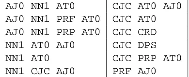
[image:2.612.307.502.15.95.2]AT0 NN1 PRP AT0 NN1 AT0 NN1
Table 1: Some of the more frequent sequences in two good clusters
the parameters it would have under an
inde-pendence assumption. The context distribution can be thought of as a distribution over a two-dimensional matrix.
The data set for all the results in this paper con-sisted of 12 million words of the British National Corpus, tagged according to the CLAWS-5 tag set, with punctuation removed.
There are 76 tags; I introduced an additional tag to mark sentence boundaries. I operate ex-clusively with tags, ignoring the actual words. My initial experiment clustered all of the tag se-quences in the corpus that occurred more than 5000 times, of which there were 753, using the -means algorithm with the -norm or city-block
metric applied to the context distributions. Thus sequences of tags will end up in the same cluster if their context distributions are similar; that is to say if they appear predominantly in similar con-texts. I chose the cutoff of 5000 counts to be of the same order as the number of parameters of the distribution, and chose the number of clusters to be 100.
To identify the frequent sequences, and to cal-culate their distributions I used the standard tech-nique of suffix arrays (Gusfield, 1997), which al-lows rapid location of all occurrences of a desired substring.
As expected, the results of the clustering showed clear clusters corresponding to syntac-tic constituents, two of which are shown in Ta-ble 1. Of course, since we are clustering all of the frequent sequences in the corpus we will also have clusters corresponding to parts of con-stituents, as can be seen in Table 2. We obvi-ously would not want to hypothesise these as con-stituents: we therefore need some criterion for fil-tering out these spurious candidates.
AJ0 NN1 AT0 CJC AT0 AJ0 AJ0 NN1 PRF AT0 CJC AT0 AJ0 NN1 PRP AT0 CJC CRD NN1 AT0 AJ0 CJC DPS
NN1 AT0 CJC PRP AT0
NN1 CJC AJ0 PRF AJ0
Table 2: Some of the sequencess in two bad clus-ters
3 Mutual Information
The criterion I propose is that with real con-stituents, there is high mutual information be-tween the symbol occurring before the putative constituent and the symbol after – i.e. they are not independent. Note that this is unrelated to Mager-man and Marcus’s MI criterion which is the (gen-eralised) mutual information of the sequence of symbols itself. I will justify this in three ways – intuitively, mathematically and empirically.
Intuitively, a true constituent like a noun phrase can appear in a number of different contexts. This is one of the traditional constituent tests. A noun phrase, for example, appears frequently either as the subject or the object of a sentence. If it ap-pears at the beginning of a sentence it is accord-ingly quite likely to be followed by a finite verb. If on the other hand it appears after the finite verb, it is more likely to be followed by the end of the sentence or a preposition. A spurious constituent like PRP AT0will be followed by an N-bar re-gardless of where it occurs. There is therefore no relation between what happens immediatly before it, and what happens immediately after it. Thus there will be a higher dependence or correlation with the true constituent than with the erroneous one.
4 Mathematical Justification
We can gain some insight into the significance of the MI criterion by analysing it within the frame-work of SCFGs. We are interested in looking at the properties of the two-dimensional distribu-tions of each non-terminal. The terminals are the part of speech tags of which there are . For each
terminal or non-terminal symbol we define
four distributions, ,
Two of these, and are just the pre-fix and sufpre-fix probability distributions for the symbol(Stolcke, 1995): the probabilities that the string derived from begins (or ends) with a
par-ticular tag. The other two for left
distribution and right distribution, are the distri-butions of the symbols before and after the non-terminal. Clearly if is a terminal symbol, the
strings derived from it are all of length 1, and thus
begin and end with , giving and a
very simple form.
If we consider each non-terminal in a SCFG,
we can associate with it two random variables which we can call the internal and external vari-ables. The internal random variable is the more familiar and ranges over the set of rules expand-ing that non-terminal. The external random vari-able, , is defined as the context in which the
non-terminal appears. Every non-root occurrence of a non-terminal in a tree will be generated by some rule , that it appears on the right hand side
of. We can represent this as where is the
rule, and is the index saying where in the right
hand side it occurs. The index is necessary since the same non-terminal symbol might occur more than once on the right hand side of the same rule. So for each , can take only those values of
! where is theth symbol on the right hand
side of .
The independence assumptions of the SCFG imply that the internal and external variables are independent, i.e. have zero mutual information. This enables us to decompose the context dis-tribution into a linear combination of the set of marginal distributions we defined earlier.
Let us examine the context distribution of all occurrences of a non-terminal with a particular
value of . We can distinguish three situations:
the non-terminal could appear at the beginning, middle or end of the right hand side. If it occurs at the beginning of a rule with left hand side ,
and the rule is#" %$'&(&(& . then the terminal
symbol that appears before will be distributed
exactly according to the symbol that occurs
be-fore , i.e. ) *,+- . The non-terminal
symbol that occurs after will be distributed
ac-cording to the symbol that occurs at the beginning of the symbol that occurs after in the right hand
side of the rule, so *.+/ *$ . By the
inde-pendence assumption, the joint distribution is just the product of the two marginals.
0
*2134+5 7689+:) <;= *$> (1)
Similarly if it occurs at the end of a rule?"
&(&(&A@B we can write it as
0
*C13D:+/ 1E139+F G@H<;= (2)
and if it occurs in the middle of a rule "
&(&(&A@B%$'&(&(& we can write it as
0
*213
+5 I+J G@H<;=K *$L (3)
The total distribution of will be the
nor-malised expectation of these three with respect to G . Each of these distributions will have
zero mutual information, and the mutual informa-tion of the linear combinainforma-tion will be less than or equal to the entropy of the variable combining them,MN G .
In particular if we have
K O+4PQ$H+:RSD+UTSVFW VYXEV
PZ[
V
R\ (4)
using Jensen’s inequality we can prove that
]
_^$9`aT b.W Vcedgf
W
V
(5)
We will have equality when the context distribu-tions are sufficiently distinct. Therefore
hB]
*<`iM2 GDj (6)
Thus a non-terminal that appears always in the same position on the right hand side of a par-ticular rule, will have zero MI, whereas a non-terminal that appears on the right hand side of a variety of different rules will, or rather may, have high MI.
Symbol Description Number of rules Most Frequent
NP Noun Phrase 107 AT0 NN1
AVP Adverb Phrase 6 AV0 AV0
PP Prep. Phrase 47 PRP NP
S Clause 19 PNP VVD NP
XPCONJ Phrase and Conj. 5 PP CJC
N-BAR 121 AJ0 NN1
S-SUB Subordinate Clause ? 58 S-SUB PP
NT-NP0AV0 3 PNP AV0
NT-VHBVBN Finite copula phrase 12 VM0 VBI
NT-AV0AJ0 Adjective Phrase 11 AV0 AJ0
NT-AJ0CJC 10 AJ0 CJC
[image:4.612.118.476.14.195.2]NT-PNPVBBVVN Subject + copula 21 PNP VBD
Table 3: Non-terminals produced during first 20 iterations of the algorithm.
5 Experimental Verification
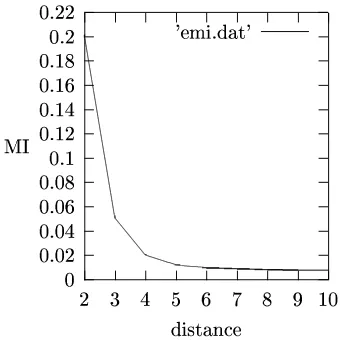
To implement this, we need some way of decid-ing a threshhold which will divide the sheep from the goats. A simple fixed threshhold is undesir-able for a number of reasons. One problem with the current approach is that the maximum likeli-hood estimator of the mutual information is bi-ased, and tends to over-estimate the mutual in-formation with sparse data (Li, 1990). A second problem is that there is a “natural” amount of mu-tual information present between any two sym-bols that are close to each other, that decreases as the symbols get further apart. Figure 1 shows a graph of how the distance between two symbols affects the MI between them. Thus if we have a sequence of length 2, the symbols before and after it will have a distance of 3, and we would expect to have a MI of 0.05. If it has more than this, we might hypothesise it as a constituent; if it has less, we discard it.
In practice we want to measure the MI of the clusters, since we will have many more counts, and that will make the MI estimate more accu-rate. We therefore compute the weighted average of this expected MI, according to the lengths of all the sequences in the clusters, and use that as the criterion. Table 4 shows how this criterion sepa-rates valid from invalid clusters. It eliminated 55 out of 100 clusters
In Table 4, we can verify this empirically: this criterion does in fact filter out the undesirable se-quences. Clearly this is a powerful technique for
k
kmlk n kmlk7o kmlk8p kmlk8q krlYs kmltsAn kmltsuo kmltsp kmltsq krln kml3n8n
[image:4.612.308.478.248.418.2]n v o w p x q y sAk z>{
|g}t~8r uj}
l
|m7
Figure 1: Graph of expected MI against distance.
Cluster Actual MI Exp. MI Valid
AT0 NN1 0.11 0.04 Yes
AT0 NP0 NP0 0.13 0.02 Yes
PRP AT0 NN1 0.06 0.02 Yes
AV0 AJ0 0.27 0.1 Yes
NN1 AT0 0.008 0.02 No
AT0 AJ0 0.02 0.03 No
VBI AT0 0.01 0.02 No
PRP AT0 0.01 0.03 No
identifying constituents.
6 Minimum Description Length
This technique can be incorporated into a gram-mar induction algorithm. We use the clustering algorithm to identify sets of sequences that can be derived from a single non-terminal. The MI cri-terion allows us to find the right places to cut the sentences up; we look for sequences where there are interesting long-range dependencies. Given these potential sequences, we can then hypothe-sise sets of rules with the same right hand side. This naturally suggests a minimum description length (MDL) or Bayesian approach (Stolcke, 1994; Chen, 1995). Starting with the maximum likelihood grammar, which has one rule for each sentence type in the corpus, and a single non-terminal, at each iteration we cluster all frequent strings, and filter according to the MI criterion discussed above.
We then greedily select the cluster that will give the best immediate reduction in descrip-tion length, calculated according to a theoreti-cally optimal code. We add a new non-terminal with rules for each sequence in the cluster. If there is a sequence of length 1 with a terminal in it, then instead of adding a new terminal, we add rules expanding that old non-terminal. Thus, if we have a cluster which con-sists of the three sequences NP, NP PRP NP
andNP PRF NP we would merely add the two rulesNP" NP PRP NP andNP" NP PRF NP,
rather than three rules with a new non-terminal on the left hand side. This allows the algorithm to learn recursive rules, and thus context-free gram-mars.
We then perform a partial parse of all the sen-tences in the corpus, and for each sentence select the path through the chart that provides the short-est description length, using standard dynamic programming techniques. This greedy algorithm is not ideal, but appears to be unavoidable given the computational complexity. Following this, we aggregate rules with the same right hand sides and repeat the operation.
Since the algorithm only considers strings whose frequency is above a fixed threshhold, the application of a rule in rewriting the corpus will often result in a large number of strings being
rewritten so that they are the same, thus bring-ing a particular sequence above the threshhold. Then at the next iteration, this sequence will be examined by the algorithm. Thus the algorithm progressively probes deeper into the structure of the corpus as syntactic variation is removed by the partial parse of low level constituents.
Singleton rules require special treatment; I have experimented with various different options, without finding an ideal solution. The results pre-sented here use singleton rules, but they are only applied when the result is necessary for the appli-cation of a further rule. This is a natural conse-quence of the shortest description length choice for the partial parse: using a singleton rule in-creases the description length.
The MDL gain is very closely related to the mutual information of the sequence itself under standard assumptions about optimal codes (Cover and Thomas, 1991). Suppose we have two sym-bols P and R that occur and times in a
corpus of length and that the sequence PER
oc-curs ( times. We could instead create a new
symbol that representsPR , and rewrite the corpus
using this abbreviation. Since we would use it
( times, each symbol would require cdgf
(
nats. The symbols P and R have codelengths of cedgf
and cedgf
, so for each pairPER that
we rewrite, under reasonable approximations, we have a reduction in code length of
2Hb cedgf
( cedgf
) cedgf
cedgf
X
PRS
X
P
X
R\
which is the point-wise mutual information be-tweenP andR .
I ran the algorithm for 40 iterations. Beyond this point the algorithm appeared to stop produc-ing plausible constituents. Part of the problem is to do with sparseness: it requires a large number of samples of each string to estimate the distribu-tions reliably.
7 Evaluation
advocated by (van Zaanen and Adriaans, 2001); i.e. use exactly the same evaluation as is used for supervised learning schemes. This proposal fails to take account of the fact that the annotation scheme used in any corpus, does not reflect some theory-independent reality, but is the product of various more or less arbitrary decisions by the an-notators (Carroll et al., 1998). Given a particular annotation scheme, the structure in the corpus is not arbitrary, but the choice of annotation scheme inevitably is. Thus expecting an unsupervised al-gorithm to converge on one particular annotation scheme out of many possible ones seems overly onerous.
It is at this point that one must question what the point of syntactic structure is: it is not an end in itself but a precursor to semantics. We need to have syntactic structure so we can abstract over it when we learn the semantic relationships be-tween words. Seen in this context, the suggestion of evaluation based on dependency relationships amongst words(Carroll et al., 1998) seems emi-nently sensible.
With unsupervised algorithms, there are two aspects to the evaluation; first how good the an-notation scheme is, and secondly how good the parsing algorithm is – i.e. how accurately the al-gorithm assigns the structures. Since we have a very basic non-lexicalised parser, I shall focus on evaluating the sort of structures that are produced, rather than trying to evaluate how well the parser works. To facilitate comparison with other tech-niques, I shall also present an evaluation on the ATIS corpus.
Pereira and Schabes (1992) establish that evaluation according to the bracketing accuracy and evaluation according to perplexity or cross-entropy are very different. In fact, the model trained on the bracketed corpus, although scoring much better on bracketing accuracy, had a higher (worse) perplexity than the one trained on the raw data. This means that optimising the likelihood of the model may not lead you to a linguistically plausible grammar.
In Table 3 I show the non-terminals produced during the first 20 iterations of the algorithm. Note that there are less than 20 of them, since as mentioned above sometimes we will add more rules to an existing non-terminal. I have taken the
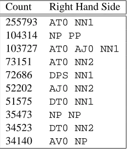
Count Right Hand Side
255793 AT0 NN1
104314 NP PP
103727 AT0 AJ0 NN1
73151 AT0 NN2
72686 DPS NN1
52202 AJ0 NN2
51575 DT0 NN1
35473 NP NP
34523 DT0 NN2
[image:6.612.350.480.14.167.2]34140 AV0 NP
Table 5: Ten most frequent rules expanding NP. Note that three of them are recursive.
liberty of attaching labels such asNPto the non-terminals where this is well justified. Where it is not, I leave the symbol produced by the program which starts with NT-. Table 5 shows the most frequent rules expanding the NP non-terminal. Note that there is a good match between these rules and the traditional phrase structure rules.
To facilitate comparison with other unsuper-vised approaches, I performed an evaluation against the ATIS corpus. I tagged the ATIS cor-pus with the CLAWS tags used here, using the CLAWS demo tagger available on the web, re-moved empty constituents, and adjusted a few to-kenisation differences (at least is one token in the BNC.) I then corrected a few systematic tagging errors. This might be slightly controversial. For example, “Washington D C” which is three tokens was tagged as NP0 ZZ0 ZZ0 where ZZ0 is a tag for alphabetic symbols. I changed the ZZ0
tags toNP0. In the BNC, that I trained the model on, the DC is a single token tagged as NP0, and in the ATIS corpus it is marked up as a sequence of threeNNP. I did not alter the mark up of flight codes and so on that occur frequently in this cor-pus and very infrequently in the BNC.
It is worth pointing out that the ATIS corpus is a very simple corpus, of radically different struc-ture and markup to the BNC. It consists primarily of short questions and imperatives, and many se-quences of letters and numbers such as T W A, A P 5 7 and so on.
For instance, a simple sentence like “Show me the meal” has the gold standard parse:
(NP (PRP me)) (NP (DT the)
(NN meal))))
and is parsed by this algorithm as
(ROOT (VVB Show) (PNP me) (NP (AT0 the)
(NN1 meal)))
According to this evaluation scheme its recall is only 33%, because of the presence of the non-branching rules, though intuitively it has correctly identified the bracketing. However, the crossing brackets measures overvalues these algorithms, since they produces only partial parses – for some sentences my algorithm produces a completely flat parse tree which of course has no crossing brackets.
I then performed a partial parse of this data us-ing the SCFG trained on the BNC, and evaluated the results against the gold-standard ATIS parse using the PARSEVAL metrics calculated by the EVALB program. Table 6 presents the results of the evaluation on the ATIS corpus, with the results on this algorithm (CDC) compared against two other algorithms, EMILE (Adriaans et al., 2000) and ABL (van Zaanen, 2000). The comparison presented here allows only tentative conclusions for these reasons: first, there are minor differ-ences in the test sets used; secondly, the CDC al-gorithm is not completely unsupervised at the mo-ment as it runs on tagged text, whereas ABL and EMILE run on raw text, though since the ATIS corpus has very little lexical ambiguity the differ-ence is probably quite minor; thirdly, it is worth reiterating that the CDC algorithm was trained on a radically different and much more complex data set. However, we can conclude that the CDC al-gorithm compares favourably to other unsuper-vised algorithms.
8 Future Work
Preliminary experiments with tags derived auto-matically using distributional clustering (Clark, 2000), have shown essentially the same results. It appears that for the simple constituents that are being constructed in the work presented here, they are sufficiently accurate. This makes the algo-rithm completely unsupervised.
I have so far used the simplest possible metric and clustering algorithm; there are much more so-phisticated hierarchical clustering algorithms that might perform better. In addition, I will explore the use of a lexicalised formalism.
This algorithm uses exclusively bottom-up in-formation; the standard estimation and parsing al-gorithms use the interaction between bottom-up and top-down information, or inside and outside probabilities to direct the search. It should be pos-sible to add this to the algorithm, though a full inside-outside re-estimation is not computation-ally feasible at the moment.
The greediness of the algorithm causes many problems. In particular, it makes the algorithm very sensitive to the order in which the rules are acquired. If a rule that rewrites AT0 NN1 is applied before a noun noun compounding rule then we will end up with lots of sequences of
NP NN1that will inevitably lead to a rule of the formNP -> NP NN1. There are possibilities of modifications that would allow the algorithm to delay committing unambiguously to a particular analysis.
9 Conclusion
In conclusion, distributional clustering can form the basis of a grammar induction algorithm, by hypothesising sets of rules expanding the same non-terminal. The mutual information criterion proposed here can filter out spurious constituents. The particular algorithm presented here is rather crude, but serves to illustrate the effectiveness of the general technique. The algorithm is computa-tionally expensive, and requires large amounts of memory to run efficiently. Though the results pre-sented here are preliminary, I have shown how an unsupervised grammar induction algorithm can induce at least part of a linguistically plausible grammar from a large mixed corpus of natural language.
Acknowledgements
This work was performed as part of the European TMR network Learning Computational
Gram-mars. I am grateful to Bill Keller, Susan
Algorithm Iterations UR UP F-score CB 0 CB `a CB
EMILE 16.8 51.6 25.4 0.84 47.4 93.4
ABL 35.6 43.6 39.2 2.12 29.1 65.0
CDC 10 23.7 57.2 33.5 0.82 57.3 90.9
CDC 20 27.9 54.2 36.8 1.10 54.9 85.0
CDC 30 33.3 54.9 41.4 1.31 48.3 80.5
[image:8.612.135.465.14.114.2]CDC 40 34.6 53.4 42.0 1.46 45.3 78.2
Table 6: Results of evaluation on ATIS corpus. UR is unlabelled recall, UP is unlabelled precision, CB is average number of crossing brackets, `' CB is percentage with two or fewer crossing brackets. The
results for EMILE and ABL are taken from (van Zaanen and Adriaans, 2001)
References
Pieter Adriaans, Marten Trautwein, and Marco Ver-voort. 2000. Towards high speed grammar in-duction on large text corpora. In Vaclav Hlavac, Keith G. Jeffery, and Jiri Wiedermann, editors, SOFSEM 2000: Theory and Practice of Informat-ics, pages 173–186. Springer Verlag.
Glenn Carroll and Eugene Charniak. 1992. Two experiments on learning probabilistic dependency grammars from corpora. Technical Report CS-92-16, Department of Computer Science, Brown Uni-versity, March.
John Carroll, Ted Briscoe, and Antonio Sanfilippo. 1998. Parser evaluation: a survey and a new pro-posal. In Proceedings of the 1st International Con-ference on Language Resources and Evaluation, pages 447–454, Granada, Spain.
Stanley Chen. 1995. Bayesian grammar induction for language modelling. In Proceedings of the 33rd An-nual Meeting of the ACL, pages 228–235.
Alexander Clark. 2000. Inducing syntactic categories by context distribution clustering. In Proceedings of CoNLL-2000 and LLL-2000, pages 91–94, Lis-bon, Portugal.
Thomas M. Cover and Joy A. Thomas. 1991. El-ements of Information Theory. Wiley Series in Telecommunications. John Wiley & Sons.
S. Finch, N. Chater, and M. Redington. 1995. Ac-quiring syntactic information from distributional statistics. In Joseph P. Levy, Dimitrios Bairaktaris, John A. Bullinaria, and Paul Cairns, editors, Con-nectionist Models of Memory and Language. UCL Press.
Dan Gusfield. 1997. Algorithms on Strings, Trees and Sequences: Computer Science and Computational Biology. Cambridge University Press.
Zellig Harris. 1954. Distributional structure. In J. A. Fodor and J. J. Katz, editors, The Structure of Lan-guage, pages 33–49. Prentice-Hall.
Sydney M. Lamb. 1961. On the mechanisation of syntactic analysis. In 1961 Conference on Ma-chine Translation of Languages and Applied Lan-guage Analysis, volume 2 of National Physical Laboratory Symposium No. 13, pages 674–685. Her Majesty’s Stationery Office, London.
W. Li. 1990. Mutual information functions ver-sus correlation functions. Journal of Statistical Physics, 60:823–837.
David M. Magerman and Mitchell P. Marcus. 1990. Parsing a natural language using mutual informa-tion statistics. In Proceedings of the Eighth Na-tional Conference on Artificial Intelligence, August.
Fernando Pereira and Yves Schabes. 1992. Inside-outside reestimation from partially bracketed cor-pora. In Proceedings of ACL ’92, pages 128–135.
Andreas Stolcke. 1994. Bayesian Learning of Prob-abilistic Language Models. Ph.D. thesis, Dept. of Electrical Engineering and Computer Science, Uni-versity of California at Berkeley.
Andreas Stolcke. 1995. An efficient probabilis-tic context-free parsing algorithm that computes prefix probabilities. Computational Linguistics, 21(2):165–202, June.
Menno van Zaanen and Pieter Adriaans. 2001. Com-paring two unsupervised grammar induction sys-tems: Alignment-based learning vs. emile. Re-search Report Series 2001.05, School of Comput-ing, University of Leeds, March.