Practical Correlated Topic Modeling and Analysis via the Rectified Anchor Word Algorithm

Proceedings of the 2019 Conference on Empirical Methods in Natural Language Processing

4991

Practical Correlated Topic Modeling and Analysis

via the Rectified Anchor Word Algorithm

Moontae Lee1 Sungjun Cho2 David Bindel2 David Mimno2

1_{University of Illinois at Chicago, Microsoft Research at Redmond}

2_{Cornell University}

[email protected], {sc782,bindel,mimno}@cornell.edu

Abstract

Despite great scalability on large data and their ability to understand correlations between top-ics, spectral topic models have not been widely used due to the absence of reliability in real data and lack of practical implementations. This paper aims to solidify the foundations of spectral topic inference and provide a practical implementation for anchor-based topic mod-eling. Beginning with vocabulary curation, we scrutinize every single inference step with other viable options. We also evaluate our matrix-based approach against popular alterna-tives including a tensor-based spectral method as well as probabilistic algorithms. Our quanti-tative and qualiquanti-tative experiments demonstrate the power of Rectified Anchor Word algorithm in various real datasets, providing a complete guide to practical correlated topic modeling.

1 Introduction

Increasing access to massive data streams is useful only if it is equipped with proper tools to discover meaningful patterns. Topic models are capable of learning low-dimensional latent structures from groups of discrete observations, while being flexi-bly applicable to a wide range of modalities without human annotations. Users can assess consumer pro-files by collecting purchase habits (Reisenbichler and Reutterer,2019), shared sentiments or topics among comments in social networks (Nguyen et al.,

2015), hidden genres/preferences on movie or mu-sic consumption (Lee et al.,2015), and latent com-munities from network snapshots (Gerlach et al.,

2018). For clarity this paper sticks to the standard terms — words, documents, and topics — but the concepts generalize to various applications beyond these examples.

Traditional algorithms for topic modeling lack scalability. To learn quality topics, probabilistic algorithms such as Variational Inference (VI) or

Markov Chain Monte Carlo (MCMC) require mul-tiple passes through the input dataset until con-vergence, and thus struggle to process millions of documents. Online or stochastic algorithms (Hoffman et al., 2010, 2013) achieve some scal-ability but at the cost of sacrificing the quality of topics. As a result, the basic Latent Dirichlet Al-location (Blei et al., 2003) is still prevalent for practitioners despite various recent advances ( Sri-vastava and Sutton, 2017; Xun et al., 2017; Xu et al.,2018). However, topics arelikely co-occur-ring termsin essence. Spectral methods explicitly construct word co-occurrence moments as statisti-cally unbiased estimators, providing alternatives to the probabilistic algorithms via moment-matching. Once the co-occurrence statistics is built with a sin-gle trivially parallelizable pass through the corpus, topic inference no longer needs to revisit individual training documents.

The Anchor Word algorithm (Arora et al.,2012,

introduce scalable implementations of the Recti-fied Anchor Word (RAW) algorithm and various evaluation metrics, investigating the impact of each inference step from vocabulary curation to topic in-ference. We also analyze quality of topics learned from annotated non-textual datasets as well as un-supervised textual corpora based on their top con-tributing words to the individual topics. To the best of our knowledge, this paper is the first com-parative study that measures both quantitative and qualitative performance across different spectral topic models and their probabilistic counterparts.

The experimental results show that the rectifi-cation step in RAW is crucial for overcoming the

model-data mismatch (Kulesza et al., 2014) but only needs a few iterations. The learned topics substantially outperform tensor-based methods and online VI, being comparable to expensive MCMC. Running RAW on a non-textual music dataset re-veals quality genre topics, whereas the probabilistic correlated model (Blei and Lafferty,2007) often learns overfitted topics that only maximize the co-occurrence of popular songs. To better support the community, we also provide scalable imple-mentations in MATLAB1 _{and Python}2 _{with full} algorithmic details in the supplementary material.

2 Spectral Topic Inference

Topic modeling assumes a document representa-tion that is sufficiently simple to allow tractable inference but also realistic to be useful. Each topic kis defined as a distributionpX_|Z(·|k)over words

wherepX_|Z(i|k)is a probability to choose a word

igiven the topick. Assuming there areN words in the vocabulary andK prepared topics, all top-ics can be compactly represented by the column-stochastic matrixB∈RN×K, where each column vectorbk∈∆N−1stands for the topick. Suppose

there areM documents in a corpus which are all written by admixing some of theseKtopics with re-spect to a certain priorf. Then topic models explain that each documentm with lengthnm is written

by: 1) Select a topic compositionwm∈∆K−1with

respect tof; 2) Writenm words by repeatedly

se-lecting a topiczfrom the compositionw_mand a wordxfrom the topicbz.

Different models adopt different priors f to better explain proper admixing of topics for the given data. For example, LDA assumes f =

1_{https://github.com/moontae/jsmf-raw}

2_{https://github.com/sc782/pyJSMF-RAW}

Dir(α) for α ∈ RK+ (Blei et al., 2003). In

correlated topic models,f=Logit-Normal(µ,Σ)

(CTM) or Probit-Normal(µ,Σ)forµ∈RK−1,Σ∈ R(K−1)×(K−1) (Blei and Lafferty, 2007;Yu and Fokoue, 2014). These models differ only in ex-plaining the stochastic generation of topic compo-sition:wm∼f. Note that entries in every column

vector b_k of B are parameters to recover in our setting, whereas probabilistic topic models often put another parametric priorg(β)from which each

b_k is sampled. The form ofgis not as crucial in learning quality topics as the form off(Asuncion et al.,2012), and can be similarly incorporated in spectral inference by putting additional regularizers when recovering eachbk(Nguyen et al.,2014).

LetH∈RN×M be the word-document matrix where the m-th column vector hm indicates the

observed term-frequencies in documentm. SayHf

is the column-normalizedH where each column ishm/nm. Topic compositions of individual

docu-ments can also be described compactly by another column-stochastic matrixW ∈RK×M whosem -th column vector iswm∈∆K−1. Then the main

learning task of topic models is to find the word-topic matrixBand topic-document matrixW that approximatesHf≈BW with the column-stochas-tic constraintsB∈ CSN×K_{,W∈ CS}K×M_{. While}

this Non-negative Matrix factorization (NMF) is identifiable under additional sparsity constraints (Huang et al.,2014), directly applying NMF meth-ods (Lee and Seung, 2001) produces incoherent topics despite small approximation errors (Stevens et al.,2012). H is too noisy and sparse to learn quality topicsBand plausible compositionsW.

2.1 Joint Stochastic Matrix Factorization

Instead of directly decomposing Hf, JSMF decomposes smaller but aggregated statistics for revealing the latent topics and their correlations. LetC ∈RN×N be the empirical word co-occur-rence matrix where Cij is the joint probability

pX₁X₂(i, j) to observe a pair of wordsiandj in

the corpus. Define the topic co-occurrence matrix

A ∈ RK×K where Akl is the joint probability

pZ₁Z₂(k, l)between two latent topicskandl. Then

JSMF transforms the topic modeling objective into a second-order NMF: C≈BABT, which is algebraically equivalent top(X1, X2|A;B) =

P

z1

P

z2p(X1|Z1;B)p(Z1, Z2|A)p(X2|Z2;B).

Definex1∈RN as a random basis vector where

only a single component corresponding to one ran-domly drawn word from the documentmis 1. Let

pmbe the vector where itsi-th component denotes

the probability for wordito occur in the document m. Thenpm=Bwm∈RN, satisfying

x1∼Categorical(pm)⇒E[x1|wm] =Bwm.

Denotenmconsecutive random draws of words by

{x1,x2, ...,xnm}, and lethm=

Pnm

t=1xt. Then

h_m∼Mult(nm,pm)⇒E[hm|wm] =nmBwm.

As explained earlier, assuming that each observed

hm follows this model does not produce

statisti-cally meaningful information toward recoveringB. Since different words in each documentmshare the same topic compositionwm, however, thecross

moments can provide useful information about co-occurring words even within a single docu-ment:E[hmhTm|wm] =E[hm|wm]E[hm|wm]T +

Cov(hm|wm) = nm(nm − 1)BwmwmTBT +

nm·diag(Bwm).Hence,

E[hmhTm|wm]−nm·diag(Bwm)

nm(nm−1)

=BwmwTmBT.

Define the co-occurrence Cm for a single

docu-mentmin terms of the observedhm:

Cm=

hmhTm−diag(hm)

nm(nm−1)

. (1)

If our observation hm follows the model, then

E[Cm|wm] =BwmwmBT by linearity of

expec-tation. Then by the Law of Iterated Expectation,

E[Cm]=Ewm[E[Cm|wm]]=BEwm[wmw

T m]BT.

We can now construct the empirical word co-oc-currence by averagingCm acrossM documents:

C:= _M1 PM_m=1Cm. Denoting the posterior

topic-topic matrix byA∗:= _M1 W WT ∈ RK×K, it is proven thatAis entry-wisely close to bothA∗and the population momentsEw_∼f[wwT]whenM is

sufficiently large (Arora et al.,2012). Thus

C ≈E[C] =B 1

M

M

X

m=1

Ewm[wmw

T m]

BT

=B_Ew_∼f[wwT]BT ≈BA∗BT ≈BABT.

Once we construct the empirical moment C

from the input data as an unbiased estimator of

the underlying generative process, JSMF enables users to recover the correctB andAup to some precision by matchingCto its posterior moments

BA∗BT. The separability assumption: every topic has one specificanchor wordthat occurs only in the context of that topic, allows the model to sat-isfy non-negative-rank(B)=rank(B)=K, guaran-teeing the existence of an identifiable factorization.

2.2 Tensor Decomposition

The separability assumption is necessary for JSMF because having only up to the second moments is not sufficient by itself to identify latent topics (Anandkumar et al.,2013). While one can release this assumption by adopting thesufficiently scat-teredcondition, it maps the factorization into an-other NP-hard optimization problem (Huang et al.,

2016). Alternatively, one can leverage third-order moments to provide sufficient statistics for identifi-able topic inference (Anandkumar et al.,2012a,b). In contrast to JSMF, tensor-based algorithms first specify f as a tractable parametric prior like the Dirichlet distribution. For example, iff= Dir(α)

withα0=Pkαk, thenE(1w_∼st_f)₍α₎[w] =α/α0, and

E(2wnd_∼f()α₎[wkwl] =

(_αk(αk+1)

α0(α0+1) (k=l)

αkαl

α0(α0+1) (k6=l)

. (2)

It makes the marginal expectations E[x1] and

E[x1xT2]further parametrized byα.

E[x1] =Ewm[x1|wm] =BE[wm] =Bα/α0

E[x1xT2] =Ewm[E[x1|wm]E[x2|wm]

T_]

=B_Ewm[wmw

T

m]BT =BE(2wnd_∼f)₍α₎B

T

Similarly we can represent up to the third moments:

E[x1⊗x2] =Ew(2nd_∼f)₍α₎[w⊗w](B,B),

E[x1⊗x2⊗x3] =Ew(3rd_∼f)₍α₎[w⊗

3_](B,B,B).

By assumingw∼Dir(α), we can fortunately at-tain closed form expressions of all three population moments only in terms ofBandα, allowing the non-central second and third moments to be fur-ther represented by lower-order moments andα0

(Anandkumar et al.,2012a). Therefore, once users construct the empirical moments given the training data and chooseα0, tensor decomposition allows

matching the empirical moments to these popula-tion moments.3_{But there are several caveats.}

First, finding such closed-form moment combi-nations is not obvious. Normally all higher-order moments are necessary for learning with the gen-eral priorf(Arabshahi and Anandkumar,2017).4 Second, _E[w⊗3]should be a diagonal tensor in order to apply the popular CP-decomposition for learning topicsB. It means that we need to assume uncorrelated topicsinstead of the separability as-sumption. Whereas most large topics models are proven indeed separable (Ding et al.,2015), users of CP-decomposition can only capture weak nega-tive correlations via the learnedαbut depending on the user choices ofα0andf= Dir. Tucker

decom-position is another option for learning correlated topics, but it instead requires additional sparsity constraints onB, demanding notably more param-eters to be estimated (Anandkumar et al.,2013). Overall, correlated topic modeling via tensor de-composition is not as flexible as using JSMF even if we factor out the trivial difference in time and space complexities.

3 The Rectified Anchor Word Algorithm

Whereas probabilistic algorithms have an intrinsic capability to fit their models on the data that does not necessarily follow their generative processes, spectral algorithms are susceptible to model-data mismatch (Kulesza et al.,2014). The Rectified An-chor Word (RAW) algorithm (Lee et al.,2015) is the first working formalism that can learn quality topics and their correlations from real data. The overall algorithm consists of five clearly divided steps: 0) construct the word co-occurrence matrix

C; 1) rectifyC; 2) find the set of anchor words

S; 3) recover the topicsB; 4) recover the topic correlationsA. Each step has various algorithmic decisions that have been previously unclear. We carefully explore other viable options, providing details on efficient implementations in the supple-mentary material.

Step 0: Create C. For spectral inference, we first construct the empirical word co-occurrence statistics as an unbiased estimator for the

under-3

JSMF does not ask users to specifyα0, flexibly and trans-parently modeling arbitrary pairwise correlations between top-ics by the co-occurrence between pairs of the corresponding anchor words.

4

They recently discover that having up to third-order mo-ments suffices to perform CP-decomposition whenfis a class of Normalized Infinitely Divisible (NID) prior.

lying generative process:C= (1/M)PM_m=1Cm

with Cm specified in Equation (1). Due to the

efficiency of anchor-based inference, the moment construction often becomes the most expensive step for large corpora, but it is trivially parallelizable as the last averaging step is the only computation that couples individual documents.

Instead of using the entire vocabulary, the stan-dard procedure is to remove stop words and prune off rare words based on either corpus frequencies or tf-idf scores. Excluding words appearing on a ma-jority of documents is also known to improve the quality of topics (Schofield et al.,2017a,b). Mea-suring the impact of vocabulary curation is not so straightforward in probabilistic topic models due to random draws in their algorithms. In contrast, spectral topic models learn topics consistently with-out any randomness. We later show how to pick the plausible size of vocabulary in the experiment section.

Step 1: RectifyC. Rectifying the co-occurrence estimator is key to successful inference as low-rank spectral learning is highly susceptible to the mismatch between the model and the data (Lee et al.,2015). ThoughC is shown to be more sta-tistically robust than Hf (Arora et al., 2012), its empirical construction from real data hardly ex-hibits the proper structures of the posterior mo-mentsBA∗BT: low-rank (LR), positive semidef-inite (PSD), nonnegative (N N), and normalized (N OR).5 _{The rectification step transforms the} noisyC into a desirable estimator by alternatingly projecting it to individual spaces (Lee et al.,2015). We also discover that cyclic Douglas-Rachford (DR) iterations can properly rectifyC, but its com-putational cost is almost twice as expensive as Al-ternating Projection (AP). Refer to the supplemen-tary material for details.

By running a truncated eigenvalue decompo-sition, the first step of AP only finds K largest eigenvaluesΛK and the corresponding

eigenvec-torsU at minimal cost. It then projectsC to the intersection ofPSDN andLRKby reconstructing

UΛ+_KUT. The next step orthogonally projects

C to N ORN by subtracting the mean average

entry-wisely from the desired total, 1.0. The nega-tive entries are then zeroed out in the subsequent projection to N NN. While the order of

projec-5

● ● ● ● ● ● ● ● ● ● ● ● ● ● ● ● ● ● ● ● ● ● ● ● ● ● ●● ● ● ● ● ● ● ● ● ● ● ●● ● ● ● ●● ● ●● Recovery Approximation Dominancy Specificity Dissimilarity Sparsity

5 10 15 25 50 100 5 10 15 25 50 100 5 10 15 25 50 100 5 10 15 25 50 100 5 10 15 25 50 100 5 10 15 25 50 100 0.65 0.70 0.75 0.80 0.85 0.90 5 10 15 1 2 3 4 0.25 0.50 0.75 −13.5 −13.0 −12.5 −12.0 −6 −5 −4 Category ● 10% 30% 50% 70% 90% NeurIPS (# documents M=1,348 / # vocabulary N=5k / average document length=380.5)

● ● ● ●● ● ● ● ● ● ● ● ● ● ● ●● ● ● ● ● ●● ● ● ● ● ● ● ● ● ● ● ● ● ● ● ● ● ● ● ● ● ● ● ● ●● ●● ● ●● ● Recovery Approximation Dominancy Specificity Dissimilarity Sparsity

5 10 15 25 50 100150 5 10 15 25 50 100150 5 10 15 25 50 100150 5 10 15 25 50 100150 5 10 15 25 50 100150 5 10 15 25 50 100150 0.76 0.80 0.84 0.88 0.92 10 15 2.5 3.0 3.5 0.2 0.4 0.6 0.8 1.0 −15.0 −14.7 −14.4 −14.1 −13.8 −7.0 −6.5 −6.0 −5.5 −5.0 Category ● 10% 30% 50% 70% 90% NYTimes (# documents M=263,325 / # vocabulary N=15k / average document length=204.9)

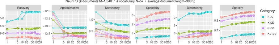
Figure 1:Vocabulary pruning assessed with AP+ADMM. A threshold of 50% implies that all words occurring in more than half of the documents are pruned. X-axis: the number of topics. Columns 1, 2, 3: lower is better / 4, 5, 6: higher is better.

● ● ● ● ●●● ●● ● ● ● ● ● ●●● ●● ● ● ● ● ● ●●● ●● ● ● ● ● ● ●●● ●● ● ● ● ● ● ●●● ●● ● ● ● ● ● ●●● ●● ● ● ● ● ● ●●● ●● ● ● ● ● ● ●●● ●● ● ● ● ● ● ●●● ●● ● ● ● ● ● ●●●_{●● ●} ● ● ● ● ●●● ●● ● ● ● ● _{● ●●● ●● ●} ● ● ● ● ●●● ●● ● ● ● ● ● ●●● ●●● ● ● ● ● ●●● ●● ● ● ● ● ● ●●●●● ● ● ● ● ● ●●● ●● ● ● ● ● ● ●●● ●● ● ● ● ● ● ●●● ●● ● ● ● ● ● ●●● ●●● ● ● ● ● ●●● ●● ● ● ● ● ● ●●● ●● ● ● ● ● ● ●●● ●● ● ● ● ● ● ●●● ●● ● Recovery Approximation Dominancy Specificity Dissimilarity Sparsity

1 5 10 20 50 100150 1 5 10 20 50 100150 1 5 10 20 50 100150 1 5 10 20 50 100150 1 5 10 20 50 100150 1 5 10 20 50 100150 0.7 0.8 6 9 12 1 2 3 0.5 1.0 −13.5 −13.0 −12.5 −12.0 −6.0 −5.5 −5.0 Categor

NeurIPS (# documents M=1,348 / # vocabulary N=5k / average document length=380.5)

Category ● ● ● ● K=5 K=20 K=50 K=100 age document length=380.5)

Figure 2:Alternating Projection (AP) vs Douglas-Rachford (DR). X-axis: the number of iterations in rectification.

AP+ADMM and◦DR+ADMM mostly agree each other and converge within 15-20 iterations. 5 iterations are often enough.

tions in each iteration does not matter, performing aN ORN-projection after the loop ends helps with

feasibility.6 _{Note that tensor-based methods have} a similar step calledwhitening, which runs a full SVD to transform the third-order moments into an orthogonal tensor for CP-decomposition.

Step 2: FindS. SayC now indicates the recti-fied co-occurrence. Then the next step is to find the anchor words. Denoting the set ofK anchor words by S ={s1, ..., sK}, the separability

as-sumption suggests: pZ₁|X₁(k′|sk) = 1 if k′ =k

andpZ_1|X₁(k′|s_k) = 0ifk′6=k. LetC be the

row-normalized version ofC. Then by the conditional independence between a pair of words given one of their topics (X1⊥X2|Z1orZ2) and separability, Cij=pX₂|X₁(j|i) =

P

k′pX₂|Z₁(j|k′)pZ₁|X₁(k′|i).

ThusCij=P_kpZ₁|X₁(k|i)Csk,j, implying that

ev-ery row vector ofC corresponding to a non-anchor word can be represented by a convex combination: P

kpZ₁|X₁(k|i) = 1of the rows{Csk}

correspond-ing to the anchor words {sk}. Therefore, the

in-ference quality depends primarily on the choice of the anchor wordsS, providing a clear metric for diagnosis. Note that rectification is also crucial for finding better anchors (Lee et al.,2015).

While using the pivoted QR (Arora et al.,2013)

6

Avoiding negative entries is useful because RAW is not a purely algebraic algorithm but uses probabilistic conditions.

substantially expedites the running time against solving a number of LPs (Arora et al.,2012), its explicit projection of each non-anchor row to the current orthogonal complement quickly damages the sparsity ofC. As a result, random projections are suggested for sizable vocabulary (Arora et al.,

2013), but such projections do not maintain the joint-stochasticity of the rectifiedC, degrading the topic quality (Lee and Mimno,2014). Instead, we develop a sparse implicit pivoted QR that requires only O(N K) space to store the basis rows and performs implicit updates inO(nnz(C)K) time without modifying any entry in the inputC.

Step 3: RecoverB. Provided with the set of an-chor wordsS and the convex coefficientsB˘ki =

{pZ₁|X₁(k|i)}, one can easily recoverBby

apply-ing Bayes’ rule: B_ik= (B˘_kici)/(PN_i′₌₁B˘ki′c_i′), whereci :=pX₁(i) is the unigram probability of

the wordi, which is equal toP_jCij. Hence the

core of this step is to find the coefficient matrixB˘

by solving a Simplex-Constrained Least Squares (SCLS) that satisfyCij=PkB˘kiCsk,jfor eachi.

While the exponentiated gradient algorithm (Exp-Grad) used in previous work (Arora et al., 2013;

● ● ●● ●● ●● ● ● ● ●● ●● ●● ● ● ● ●● ●● ●● ● ● ● ●● ● ● ●● ● ● ● ● ● ●● ●● ● ● ● ●● ●● ●● ● Approximation Dominancy Specificity Dissimilarity Coherence Sparsity

5 10 15 20 25 5 10 15 20 25 5 10 15 20 25 5 10 15 20 25 5 10 15 20 25 5 10 15 20 25 0.5 0.6 0.7 0.8 0.9 −320 −280 −240 −200 −160 0 5 10 15 0 1 2 3 0.00 0.25 0.50 0.75 1.00 −12.5 −10.0 −7.5 −5.0 Category ● 1.Baseline 2.OVI 3.Tensor 4.AP+ExpGrad 5.Gibbs NeurIPS (# documents M=1,348 / # vocabulary N=5k / average document length=380.5)

● ● ●● ●● ●● ● ● ● ● ● ● ● ● ● ● ● ● ●● ● ● ● ● ● ● ● ● ● ● ● ●● ● ● ● ● ● ● ● ● ● ● ● ● ● ● ● ● ● ● ● Approximation Dominancy Specificity Dissimilarity Coherence Sparsity

5 10 15 20 25 5 10 15 20 25 5 10 15 20 25 5 10 15 20 25 5 10 15 20 25 5 10 15 20 25 0.6 0.7 0.8 −350 −300 −250 4 8 12 0 1 2 3 0.25 0.50 0.75 1.00 −10 −5 Category ● 1.Baseline 2.OVI 3.Tensor 4.AP+ExpGrad 5.Gibbs Blog (# documents M=11,321 / # vocabulary N=4,447 / average document length=161.3)

● ● ●● ●● ●● ● ● ● ● ● ● ● ● ● ● ● ● ● ● ●● ●● ● ●● ●● ●● ● ● ● ● ● ● ● ● ● ● ● ● ● ● ● ● ● ● ● ● ● Approximation Dominancy Specificity Dissimilarity Coherence Sparsity

5 10 15 20 25 5 10 15 20 25 5 10 15 20 25 5 10 15 20 25 5 10 15 20 25 5 10 15 20 25 0.6 0.7 0.8 −500 −450 −400 −350 3 6 9 0 1 2 3 0.00 0.25 0.50 0.75 1.00 −12.5 −10.0 −7.5 −5.0 Category ● 1.Baseline 2.OVI 3.Tensor 4.AP+ExpGrad 5.Gibbs Yelp (# documents M=17,089 / # vocabulary N=1,606 / average document Length=36.4)

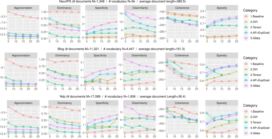
Figure 3:Quantitative results from various methods. Tensor (CP-decomposition (Anandkumar et al.,2012a)) performs better than the Baseline (Anchor Word algorithm with ExpGrad without any rectification (Arora et al.,2013)) and OVI (Online Variational Inference (Hoffman et al.,2010)), but much poorer than the AP+ExpGrad (AP-rectified Anchor Word algorithm (Lee et al.,2015)) and Gibbs (Collapsed Gibbs Sampling (Yao et al.,2009)). Surprisingly the tensor algorithm does not show consistent behavior for increasing number of topics in X-axis. Closer to Gibbs is generally better in Y-axis.

of Multipliers (ADMM), which is not sensitive to different parameter settings. Note that we also pro-vide the Active-Set method that can solve SCLS within machine precision in our implementation, but our practical choice is ADMM due to the much higher cost of running the Active-Set method.

Step 4: Recover A. The final step is to re-cover the topic correlation matrix A, which summarizes the latent topic compositions W

by A= (1/M)W WT. Instead of learning W, Anchor Word algorithms learn the correlationsA

by again leveraging the separability assumption: P

l′ P_k′pX₁|Z₁(sk|k′)pZ₁Z₂(k′, l′)

pX₂|Z₂(sl|l′) =pX_1|Z₁(s_k|k)

P

l′pZ₁Z₂(k, l′)pX_2|Z₂(s_l|l′)

=pX₁|Z₁(sk|k)pZ₁Z₂(k, l)pX₂|Z₂(sl|l). Thus

pZ₁Z₂(k, l)=pX−₁1_|Z₁(sk|k)pX₁X₂(sk, sl)pX−₂1_|Z₂(sl|l),

which can be simplified to A =B_S−_∗1CSSBS−∗1. Therefore the co-occurrence of the anchor words sk and sl transparently captures the correlation

between the pair of topics k and l. Note that the anchor words are generally rare words — in order to be the vertices of an underlying convex hull of the word co-occurrence space — whose co-occurrences are even rarer and noisier. The rectification step in JSMF effectively balances these entries (Lee et al.,2015), thereby realizing robust and transparent correlated topic inference.

4 Experimental Results

We evaluate our models of interest on two standard textual corpora: NeurIPS and NYTimes. Full pa-pers in NeurIPS are generally longer but share a smaller vocabulary (12k), whereas massive news articles in NYTimes have medium length with the largest vocabulary (103k). Due to high complexi-ties of tensor decomposition, we prepare two small textual datasets: Blog and Yelp. They consist of po-litical blogs (Eisenstein et al.,2011) and business reviews (Lee and Mimno, 2014) with the small-est vocabulary (4.4k, 1.6k), respectively. In addi-tion, we adopt two non-textual preference datasets: Movies and Songs. They include 10m movie re-views7and music playlists from Yes.com.8 In con-trast to textual datasets, we can retrieve genre infor-mation for Movies and Songs.9 You can find the exact statistics of each dataset in our figures.

Evaluating topic models with held-out likeli-hoods or perplexities only is often misleading (Passos et al.,2011;Lee and Mimno, 2014). In-stead we follow six metrics used on (Lee et al.,

7_{Movies has a vocabulary of 10.7k movies. https://} grouplens.org/datasets/movielens/10m/

8

Songs has a vocabulary of 75.3k songs. http:// csinpi.github.io/lme/data_page.html

9

● ● ● ● ● ● ●● ● ● ● ● ● ● ● ● ● ● ●● ● ● ● ●● ● ●● ●● ● ● ● ●● ● ● ● ● ● ● ●● ● ● ● ● ● ● ● ● ●● ● ● ● ●●●● Approximation Dominancy Specificity Dissimilarity Coherence Sparsity

5 10 15 25 50 100150 5 10 15 25 50 100150 5 10 15 25 50 100150 5 10 15 25 50 100150 5 10 15 25 50 100150 5 10 15 25 50 100150 0.76 0.80 0.84 0.88 0.92 −350 −300 10 15 1 2 3 4 0.2 0.4 0.6 0.8 1.0 −14.5 −14.0 Category ● 1.AP+ActiveSet 2.AP+ADMM 3.AP+ExpGrad 4.Gibbs NYTimes (# documents M=263,325 / # vocabulary N=15k / average document length=204.9)

● ● ● ● ● ● ● ● ● ● ● ● ● ● ●● ● ● ●● ● ● ● ● ● ● ● ● ● ● ●● ● ● ● ●● ● ● ● ● ● ●● ● ● ● ● Approximation Dominancy Specificity Dissimilarity Coherence Sparsity

5 10 15 25 50 100 5 10 15 25 50 100 5 10 15 25 50 100 5 10 15 25 50 100 5 10 15 25 50 100 5 10 15 25 50 100 0.75 0.80 0.85 0.90 −240 −220 −200 −180 −160 −140 5 10 15 2 3 4 0.1 0.2 0.3 0.4 0.5 0.6 −12.5 −12.0 −11.5 −11.0 Category ● 1.AP+ActiveSet 2.AP+ADMM 3.AP+ExpGrad 4.Gibbs Movies (# documents M=63,041 / # vocabulary N=10k / average document Length=142.8)

● ● ● ● ● ● ● ● ● ● ● ● ● ● ● ● ● ● ● ●● ● ●● ● ● ● ● ● ● ● ● ● ●● ● ● ● ● ● ● ● ●●● ● ● ● Approximation Dominancy Specificity Dissimilarity Coherence Sparsity

5 10 15 25 50 100 5 10 15 25 50 100 5 10 15 25 50 100 5 10 15 25 50 100 5 10 15 25 50 100 5 10 15 25 50 100 0.75 0.80 0.85 0.90 −500 −400 −300 −200 0 5 10 15 20 0 2 4 0.6 0.7 0.8 0.9 −12.8 −12.4 −12.0 −11.6 Category ● 1.AP+ActiveSet 2.AP+ADMM 3.AP+ExpGrad 4.Gibbs Songs (# documents M=14,653 / # vocabulary N=10k / average document length=119.2)

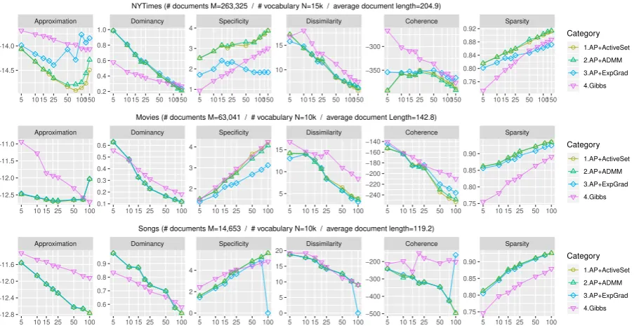
Figure 4:ExpGrad vs ADMM vs ActiveSet. Our△AP+ADMMand◦AP+ActiveSetalgorithms outperform the previous state-of-the-art rectified algorithm⋄AP+ExpGrad, being more comparable to probabilistic▽Gibbssampling. Columns 1, 2: lower is better / 3, 4, 6: higher is better / 5: closer to Gibbs is better.

2015) for fair and comprehensive evaluations. Recovery (_N1 P_ikCi − P_kB˘kiCskk2)

evalu-ates how successfully anchor words reconstruct the word co-occurrence space. Approximation (kC − BABTkF) measures the closeness

be-tween the learned factorization and the unbiased co-occurrence statistics. Note that they are measured againstthe originalC rather than the rectified one, and are visualized in logarithms of base 1.8 for readability. Dominancy (_K1 P_kAkk)is the

aver-age self-correlations, indirectly gauging the loss of correlations between different topics. Speci-ficity(_K1 P_kKL(bk||PiC∗i)) measures the

aver-age KL-distance of each topic from the unigram distribution of the corpus.Dissimilaritycounts the mean number of top words in each topic that do not belong to the top 20 words of other topics. Co-herence(_K1 P_kPx1,x2∈T opk

x16=x2 log

D2(x1,x2)+ǫ

D1(x2) )

pe-nalizes any pair of top words in each topic that do not appear together in the training documents.10 While we report Coherence, the metric could be deceptive if a model learns many duplicated topics whose top words are mostly frequent words (Huang et al.,2016). Thus following the trends of Gibbs generally implies better performance. We newly add Sparsity (_K1 P_k

√

N−(kbkk1/kbkk2)

√

N−1 ) (Hoyer, 2004) to gauge the average sparsity of the topics.

10

D2(x1, x2) means the number of training documents where two wordsx1andx2jointly appear.D1(x2)counts the number of training documents that include the wordx2.

Vocab pruning: We experiment different docu-ment frequency cut-offs. Figure1shows that re-moving all the words that occur more than 10% the documents is too aggressive, thus showing incon-sistent behavior as the number of topics grows. In contrast, using 90% cut-off saves too many words. We process vocabulary identically to (Lee et al.,

2015) for fair comparison, discarding the words that appear in more than 50% of the documents. The title on top of each figure indicates the size of the pruned vocabulary with the specific statistics.

Quantitative analysis: After constructing C

(Step 0), the Baseline method (Arora et al.,2013) skips to finding the anchor words (Step 2) without any rectification. While we use the exponentiated gradient (ExpGrad) method adopted in the previous work (Arora et al.,2013), we do not perform any random projection or pseudo-inverse recovery of

Ain order to prevent further degradation of learn-ing quality. For methods within the framework of JSMF, we execute 150 iterations of AP or DR recti-fications (Step 1) , which is equivalent to (Lee et al.,

2015). However, Figure2shows that running only 5 iterations of AP or DR sufficiently rectifiesC, and 15-20 iterations yields almost identical results to 150 iterations.

0 1

.01.022 .023 .034 .025 .086 .067 .038 .059 .0810.1311 12.11.0613.0314.2715 Blues

Classical Easy/Newage Electronic Folk/Country Hip-Hop/Rap Jazz Latin Other Pop R&B/Soul Reggae Rock

0 1

.51.032 .033 .034 .055 .126 .047 .018 .029 .0110.0011.0512.0213.0314.0615

Figure 5:AP+ADMM (left) vs CTM (right). Thecolumn 0shows the genre distribution of the entire corpus. Each column 1-15 stands fork-th topic where two most prominent genres are oforangecolors. The size of each box is proportional to the relative intensity. Fractional value below each topic number on the X-axis indicates the marginal probabilitypZ₁(k)of the latent topick.

AP+ADMM learns better topics that capture more coherent information about music genres.

the quality of topics. For ExpGrad, we set the learn-ing rate as 50.0, which is the best-known from (Lee et al.,2015). For our ADMM, we setλ= 1.9and γ= 3.0, but we also find that the algorithm is not at all sensitive to different settings. For probabilistic inference, we adopt a sufficiently mixed collapsed Gibbs Sampling (Gibbs) from the standard Mallet library11, using 1,000 iterations after discarding the initial 200 burn-in samples. We also run Online Variational Inference (OVI) (Hoffman et al.,2010) in the standard Gensim package. Finally, we run CP-decomposition for the Tensor algorithm.12

Figure3shows that Tensor decomposition out-performs Baseline and OVI, but evaluation met-rics fluctuate as the number of topics increases. We also observe that the topic distribution given a word becomes closer to uniform over growing num-ber of topics. In contrast, AP+ExpGrad exhibits consistent behaviors as expected in spectral infer-ence, being most comparable to Gibbs. Though SCLS (Step 3) is a convex problem, Figure4shows that AP+ADMM and AP+ActiveSet improve Speci-ficity and Sparsity over AP+ExpGrad, making the learned topics even more comparable to Gibbs. We choose ADMM as our main optimization method especially because it is not only insensitive to its parameters, but also notably faster than ActiveSet. Users of ExpGrad must search through less intu-itive learning rates for optimal performance, which can be different for each dataset.

11

Gibbs is run on Java Mallet that implements time- and memory-efficient sampling with optimized multicore controls.

12

https://github.com/FurongHuang/ TensorDecomposition4TopicModeling

Qualitative analysis: We first verify the learned topics in the NeurIPS dataset. As given in Figure

6, AP+ADMM and Gibbs learn comparable topics, while the topics learned from OVI and Tensor are not sufficiently separated: OVI repeats ‘cell’ and ‘neuron’ in different topics. Similarly, ‘neuron’ and ‘layer’ contribute to nearly every topic in Tensor

regardless of hidden differences in their themes.

When running Variational CTM (Blei and Laf-ferty,2007) with default parameters, the resulting topics do not show distinguishable genre associa-tions. Most topics involve Pop and Rock, emulating the overall genre distribution of the corpus as illus-trated in Figure5. In contrast, our AP+ADMM cap-tures three Jazz topics (T1: Electronic, T5: Pure, T9: Blues style) and four specific Rock topics (T3: Folk Rock, T4: Rock n Roll, T12: Pop style, T15: Alternative Rock). While both models discover Reggae and Latin genres, CTM’s associate more with generic Other genres, whereas AP+ADMM’s associate more with Folk/Country or Pop.

OVI (Hoffman et al.,2010) AP+ADMM (This paper)

cell layer object neuron node neuron circuit synaptic cell layer layer neuron node output rbf control action dynamic optimal controller image cell filter neuron vector recognition layer hidden word speech neuron cell object map activity cell field visual direction image

cell object recognition layer vector gaussian noise hidden approximation matrix

Tensor (Anandkumar et al.,2012a) Gibbs (Yao et al.,2009)

cell neuron field visual direction neuron cell visual signal response

layer hidden neuron field approximation control action policy optimal reinforcement object image layer recognition field recognition image object feature word neuron layer hidden threshold synaptic hidden net layer dynamic neuron

hidden noise gaussian layer approximation gaussian approximation matrix bound component

● ●

● ●

● ●

● ● NeurIPS

5 10 15 25 50 100 1.0

1.5 2.0

● ● ●

● ● ● ●

●● ● NYTimes

5 10 15 25 50 100150 2.0

2.5 3.0 3.5 4.0

Figure 6:(Left) Each line consisted of top 5 words represents a topic from NeurIPS (K= 5). Both OVI and Tensor tend to repeat top words across different topics, whereas AP+ADMM discovers distinctive and meaningful topics similar to Gibbs. (Right) Scalability of the methods measured inlog10(seconds). Compared to◦OVIand▽Gibbs, our△AP+ADMMcan infer quality topics while being more scalable to large corpora.

share a genre-specific theme, people often watch and review recently released movies rather than coherently consume movies within related genres. Thus topics inferred from Movies consist of year-specific topics as well as Fantasy or Sci-Fi.

5 Discussion

Runtime analyses on RAW alongside other meth-ods demonstrate its strong scalability. In our ex-periment, the tensor algorithm takes 5 hours for learning 5 topics on NeurIPS and 48 days for 25 topics on Yelp. It runs indefinitely for 20-25 topics on Blog, which explains two missing data points in Figure3. Topic learning with RAW takes less than a minute on these toy datasets and less than an hour on the largest NYTimes when using 15 iterations of AP with ADMM.

Two plots in Figure6further verify that RAW with AP+ADMM is approximately 4 times faster than OVI (in addition to learning better topics), and 40 times faster than Gibbs (but showing com-parable results across various numbers of topics) on the NYTimes dataset. While OVI runs faster on NeurIPS, the superior quality of topics inferred with RAW far outweighs the additional cost. As running the entire pipeline of RAW takes less than 5 minutes in NeurIPS, OVI is not as competitive as RAW.13 Lastly, the Variational CTM takes 15 minutes to learn 15 topics on Songs, but 6 hours for 50 topics. In contrast, our RAW method takes less than 10 minutes to find 50 topics on Songs.

13_{Note that slight fluctuations in Figure6are due to the}

load-balancing from the job queue on our high-performance computing cluster. For precision, we draw these two panels by averaging the running times from 10 different trials.

6 Conclusion

By removing the dependency on the training doc-uments, spectral topic modeling provides scal-able formalisms for finding compact high-level structures in sparse and discrete data such as text and user-preference. The Rectified Anchor Word (RAW) algorithm enjoys its transparent and con-sistent behaviors, working seamlessly on various types of textual and non-textual real datasets. In particular, our AP+ADMM algorithm outperforms the previous AP+ExpGrad (Lee et al.,2015), be-ing more comparable to Gibbs samplbe-ing and less sensitive to parameters.

Through this paper, we closely investigate each step of inference with various algorithmic deci-sions. Proper pruning of vocabulary is shown neces-sary, and rectification is proven crucial for reliable topic inference under the model-data mismatch. Joint Stochastic Matrix Factorization (JSMF) with the rectification better models arbitrary pairwise topic correlations at lower cost than probabilistic correlated topic model and tensor decomposition. We hope that our work, built upon the theoreti-cal insights on spectral inference, provide a com-plete guide to correlated topic modeling for both researchers and practitioners.

Acknowledgements

References

Anima Anandkumar, Dean P. Foster, Daniel Hsu, Sham Kakade, and Yi-Kai Liu. 2012a. A spectral algo-rithm for latent Dirichlet allocation. InNIPS.

Animashree Anandkumar, Daniel J. Hsu, Majid Janza-min, and Sham Kakade. 2013. When are overcom-plete topic models identifiable? uniqueness of tensor tucker decompositions with structured sparsity.

Animashree Anandkumar, Sham M Kakade, Dean P Foster, Yi-Kai Liu, and Daniel Hsu. 2012b. Two svds suffice: Spectral decompositions for probabilis-tic topic modeling and latent dirichlet allocation.

F. Arabshahi and A. Anandkumar. 2017. Spectral meth-ods for correlated topic models.AISTATS.

S. Arora, R. Ge, and A. Moitra. 2012. Learning topic models – going beyond SVD. InFOCS.

Sanjeev Arora, Rong Ge, Yonatan Halpern, David Mimno, Ankur Moitra, David Sontag, Yichen Wu, and Michael Zhu. 2013. A practical algorithm for topic modeling with provable guarantees. InICML.

Arthur U. Asuncion, Max Welling, Padhraic Smyth, and Yee Whye Teh. 2012. On smoothing and infer-ence for topic models. CoRR, abs/1205.2662.

D. Blei and J. Lafferty. 2007. A correlated topic model of science. Annals of Applied Statistics.

D. Blei, A. Ng, and M. Jordan. 2003. Latent Dirichlet allocation.JMLR.

Weicong Ding, Prakash Ishwar, and Venkatesh Saligrama. 2015. Most large topic models are ap-proximately separable. In ITA, 2015, pages 199– 203. IEEE.

Jacob Eisenstein, Duen Horng Chau, Aniket Kittur, and Eric P. Xing. 2011. Topicviz: Semantic navigation of document collections. CoRR, abs/1110.6200.

Martin Gerlach, Tiago P. Peixoto, and Eduardo G. Alt-mann. 2018. A network approach to topic models.

Science Advances, 4(7).

Matthew D. Hoffman, David M. Blei, and Francis Bach. 2010. Online learning for latent dirichlet allocation. InNIPS.

Matthew D Hoffman, David M Blei, Chong Wang, and John Paisley. 2013. Stochastic variational infer-ence. The Journal of Machine Learning Research, 14(1):1303–1347.

Patrik O. Hoyer. 2004. Non-negative matrix factoriza-tion with sparseness constraints.JMLR.

K. Huang, N. D. Sidiropoulos, and A. Swami. 2014. Non-negative matrix factorization revisited: Unique-ness and algorithm for symmetric decomposition.

IEEE Transactions on Signal Processing.

Kejun Huang, Xiao Fu, and Nikolaos D. Sidiropoulos. 2016. Anchor-free correlated topic modeling: Iden-tifiability and algorithm. InNIPS.

Alex Kulesza, N Raj Rao, and Satinder Singh. 2014. Low-rank spectral learning. InAISTATS.

Daniel D. Lee and H. Sebastian Seung. 2001. Al-gorithms for non-negative matrix factorization. In

NIPS.

Moontae Lee, David Bindel, and David Mimno. 2015. Robust spectral inference for joint stochastic matrix factorization. InNIPS.

Moontae Lee and David Mimno. 2014. Low-dimensional embeddings for interpretable anchor-based topic inference. In EMNLP. Association for Computational Linguistics.

Zita Marinho. 2015. Moment-based algorithms for structured prediction.

Thang Nguyen, Yuening Hu, and Jordan Boyd-Graber. 2014. Anchors regularized: Adding robustness and extensibility to scalable topic-modeling algorithms. InACL.

Thien Hai Nguyen, Kiyoaki Shirai, and Julien Velcin. 2015. Sentiment analysis on social media for stock movement prediction. Expert Systems with Applica-tions, 42(24):9603 – 9611.

Alexandre Passos, Hanna Wallach, and Andrew McCal-lum. 2011. Correlations and anticorrelations in lda inference. InNIPS.

Martin Reisenbichler and Thomas Reutterer. 2019. Topic modeling in marketing: recent advances and research opportunities. Journal of Business Eco-nomics, 89(3):327–356.

Alexandra Schofield, M˚ans Magnusson, and D Mimno. 2017a. Understanding text pre-processing for la-tent dirichlet allocation. InProceedings of the 15th conference of the European chapter of the Associa-tion for ComputaAssocia-tional Linguistics, volume 2, pages 432–436.

Alexandra Schofield, M˚ans Magnusson, and David Mimno. 2017b. Pulling out the stops: Rethinking stopword removal for topic models. InProceedings of the 15th Conference of the European Chapter of the Association for Computational Linguistics: Vol-ume 2, Short Papers, pages 432–436.

Akash Srivastava and Charles A. Sutton. 2017. Autoen-coding variational inference for topic models. In

ICLR.

Keith Stevens, Philip Kegelmeyer, David Andrzejew-ski, and David Buttler. 2012. Exploring topic co-herence over many models and many topics. In

Hongteng Xu, Wenlin Wang, Wei Liu, and Lawrence Carin. 2018. Distilled wasserstein learning for word embedding and topic modeling. InAdvances in Neu-ral Information Processing Systems 31, pages 1716– 1725.

Guangxu Xun, Yaliang Li, Wayne Xin Zhao, Jing Gao, and Aidong Zhang. 2017. A correlated topic model using word embeddings. InProceedings of the 26th International Joint Conference on Artificial Intelli-gence, IJCAI’17, pages 4207–4213.

Limin Yao, David Mimno, and Andrew McCallum. 2009. Efficient methods for topic model inference on streaming document collections. InKDD.