A Unified Approach to Computing
Distributions Associated with Hidden State
Sequences
Donald E. K. Martin and John A. D. Aston
Abstract— In this paper a method is given for computing distributions of statistics of hidden state sequences. The method applies to any situation for which the conditional distribution of states given observations may be modeled by a factor graph with factors that depend on current and past states but not future ones. Model structure is exploited to develop a Markov chain that facilitates efficient computation of distributions. The methodology may be used for discrete hidden state sequences perturbed by noise and/or missing values, and for state sequences that serve to classify observations. Two detailed examples are given to illustrate the computational procedure.
Index Terms—Auxiliary Markov chain, classification, deterministic finite automaton, distribution of pattern statistics, hidden state sequences.
I. INTRODUCTION
An important problem in structured learning is the prediction of values of a sequence of hidden states, conditioned on observed data. A typical choice for this task is to maximize the conditional probability of states given the data and the model (producing the Viterbi sequence; see [1]). Whereas this method of prediction is optimal in many situations, it may not be so if one is mainly interested in inference on statistics of the hidden states. Determining sampling distributions associated with statistics of hidden states is the topic of the present paper.
In classification, runs in hidden labels correspond to regimes in the observed data. Examples of applications where statistics of regimes are of interest are [2], in the context of business cycle analysis, and [3] and [4], which classified DNA nucleotides to locate genes or CpG islands, respectively. Hidden states can also be the true values of noisy data with or without missing values. In that situation, any pattern of interest in the observed data is of relevance in the hidden states as well. Prototypical applications include microarray experiments, which frequently have noisy data for various experimental reasons [5], and noisy time series data [6].
Manuscript received July 2, 2008. This work was supported in part by the National Science Foundation Grant DMS-0805577.
Donald E. K. Martin is with the Department of Statistics, North Carolina State University, Raleigh, NC 27695, USA (phone: 919-515-1936; fax: 919-515-1169; e-mail: martin@ stat.ncsu.edu).
John A. D. Aston is with CRISM, Department of Statistics, Warwick University, UK (e-mail: [email protected]).
In [7] an illustration is given of the pitfalls of basing inference for functions of hidden states on the Viterbi sequence, and a method based on Markov chains is presented to compute exact sampling distributions of statistics of patterns in states of hidden Markov models. In this paper that methodology is extended to more general settings, as it is applied to both discriminative and generative models for which the conditional distribution of states given observations can be represented as a factor graph with factors that depend on current and past states but not future ones. This is important because it supplies a way to analyze data from a variety of models, supplanting the need to develop new methodology for each individual case. In addition, the development of the auxiliary Markov chain used for computations is made more efficient through the use of deterministic finite automata, in the sense that in some cases the number of states needed in the auxiliary Markov chain is reduced.
After background information is given on the model framework, details of the computational procedure are presented, along with two examples. The final section is a conclusion.
II. THE MODEL
Let o=( ,o1…,oT) be a sequence of observations, and
1 ( ,s ,sT) =
s … the corresponding hidden states, with each st
from a finite state space Σ. The conditional distribution of states given observations is assumed to factor according to
( )
0 1
1 1
( ) ( , ) ( , , )
( )
T h
S m t
t m
p s s
Z = +
= Ψ
∏
Ψs o o o
o st . (1)
In (1), ( )h t
s are history variables for time (or sequence location) that include t st m− and some subset of st m− + −1:t 1 (sa b: =s sa, a+1,…,sb, a≤b), so that the sequence has m-th
order dependence . Also, sm ≡s1:m are initialization states.
(In general, st ≡st m− +1:t, t=m m, +1,…,T ). The factors 0
Ψ and Ψ1 are non-negative potential functions that indicate compatibility between the states that are their arguments and some subset (which is possibly empty) of the observations o. These functions are (or contain) parameters that are estimated from data. The partition function is a normalization constant, so that (1) defines a probability distribution.
( )o
The representation (1) is fairly general in that conditional probabilities from various graphical models take that form. The model is a special case of a conditional random field (CRF) [8]. When ( )
1
h
t t
s =s− , the model is a linear chain CRF,
and a linear chain CRF with vector states is a dynamic conditional random field [9]. The model (1) can also be applied to generative models for the joint distribution of states and observations. For example, a hidden Markov model (HMM)
0 1 1 1 1
1 1 1 1 2 2 1 ( , ) ( , , )
( , ) ( ) ( ) ( ) ( )
t t t T
t t t t
t
s o s s o
p g s γ o s g s s o s
−
− =
Ψ Ψ
=
∏
s o γ
has a conditional distribution (p s o) given by (1), with , potential functions and as indicated, and . Dynamic Bayesian networks [10] may be represented as an HMM with vector states, and thus also satisfy (1). Other models may also be represented as (1) as well.
1
m= Ψ0 Ψ1
( ) ( , )
Z =
∑
ps
o s o
The computation of is facilitated by the backward variables, defined by
( )
Z o
( , ) 1
T sT
β o ≡ for all sT , and
for t T ,
, which lend themselves to recursive computation: . Using the
backward variables, is obtained as
1:
( ) 1 1
( , ) ( , , )
t T
T h
t st s τ t sτ sτ
β
+ = +
≡
∑ ∏
Ψo o = −1,T−2
s o ,m
…
1
( ) 1 1 1 1 1
( , ) ( , ) ( , , )
t
h
t st s t st st t
β β
+ + + + +
≡
∑
Ψo o
( )
Z o
0
( ) ( ) ( )
m m m m
s
Z o =
∑
Ψ s β s .The model (1) has a Markovian property that is useful. For ,
1
t≥ +m
1:
:
1: 1: 1
1: 1
( )
( )
( , )
( ) (
t T
t T S s
S t
S t t
S t s S
p p s
p s s
p s p
+
−
−
= =
∑
∑
s o o
o
o so) ( )
1
1 1 1
( , , ) ( , )
( ,
( , )
h
t t t t
S t t
t t
s s s
p s s s
β
β −
− −
Ψ
= o o = o
o ). (2)
Thus conditioned on the observations, transition probabilities in the state sequence given all previous states depend on only the last m states. This Markovian structure is exploited in the next section to develop an auxiliary Markov chain (AMC)
that eases the computation of conditional distributions of statistics of s.
{ }
T mYτ τ=
III. COMPUTATION OF DISTRIBUTIONS IN HIDDEN STATE
SEQUENCES
Terminology related to patterns is now given as a prelude to a description of the computational algorithm.
A. Preliminary notation and terminology
The alphabet is a nonempty finite set whose elements are called letters. A word over is a sequence of letters, and its length
Σ
w Σ
w is the number of letters forming the word. The word of length zero is denoted by ε. , is the
set of all words formed by taking k letters from
k
Σ k≥0
Σ, with
{ }
0 ε
Σ = . The set of all words over Σ is denoted by Σ* ;
* 0 1 2
Σ = Σ ∪ Σ ∪ Σ ∪… Let Σ ≡≤j
{
w∈ Σ*:w ≤ j}
. For words u and over v Σ, the concatenation is the word formed by adding v to the end of u. A word v is called a suffix of u if
uv
u=wv for some , and v is a prefix of if
* w∈ Σ
u u=vw, w∈Σ*. For w∈ Σ*, define w( )j to be the longest j
v∈Σ≤ that is a suffix of w. Finally, a pattern L is any subset of Σ*
.
B. Markov chain embedding
Distributions associated with patterns and statistics in a state sequence may be computed through an auxiliary Markov chain (AMC) that sequentially processes each random variable of the sequence and returns probabilities for each of the states of the chain. This technique was formalized in [11], and has been used extensively, including in [12] and [13] to compute generalized sooner and later waiting time distributions of collections of patterns that have to occur pattern specific numbers of times, and, as stated earlier, in [7], where distributions of patterns in state sequences of HMMs are computed.
The work of the latter reference is extended here to more general factor graphs of the form (1). The AMC that is formed for computation is of the form ( , )Φθ , where θ is a vector holding the statistic(s) of interest, and Φ is a set of supplementary variables needed to form the Markov chain.
Φ consists of the variable q that gives progress into the pattern of interest, an m-tuple st that holds the last m
values of s1:t, and possibly other variables, though no other
variables are used in Φ in the remainder of this paper. Deterministic finite automata assist with setting up possible values of in an efficient manner. q
A deterministic finite automaton (DFA) is a five-tuple,
D
(
, , , 0,)
D= Q Σδ q F , where Q is a finite set of automaton states, Σ an alphabet, δ:Q×Σ →Q a transition function, q0 an initial state, and F a set of final states. The transitions of a DFA may be represented as a directed graph with labeled edges, where an arrow labeled with the character
a∈ Σ connecting a state to a state r is drawn provided that
q
( , )q a r
δ = .
A state r∈Q is accessible if there is a path from to , and coaccessible if there exists a path from r to one of the final states. The automaton recognizes all words that can be formed by concatenating from left to right the labels of edges visited by any path over its transition graph that starts at and ends at a state of
0
q r
0
q
F.
procedure of [15], which involves determining equivalence classes for states Q of D based on its transitions, and defining a minimal automaton Dmin with states that
correspond to equivalence classes. Values of correspond to states of
q
min
D .
An -th order automaton ([16]) may be formed by coupling words of with states of , and then deleting any states that are not accessible and coaccessible. Elements
of Φ are then states of .
m D( )m m
≤
Σ Dmin
( , )q st D( )m
The variables of Φ and of θ at any time t are uniquely determined from s1:t, and thus, so are initial and transition
probabilities of the AMC
{ }
Yτ τT=m. If (qm,θ
m) are the values of and q θ determined from sm, then[ m ( m, m, m)] S( m
P Y = q s θ =p s o)
1:
1 0
( ) ( ) ( , ) ( , )
m T
S m
s
p Z s β s
+
−
⎡ ⎤
=
∑
s o = ⎣ o ⎦Ψ o m m ot
, (3)
and if ( ,q s′ t−1,
θ
′ →) ( , , )q sθ
with the occurrence of st attime , t
1 1
[ t ( , , )t t ( , t , )] ( t t 1) P Y = q s θ Y− = q s′ − θ′ = p s s− . (4)
Equations (3) and (4) lead to a recursive method for computing
ψ
t( , , )q sθ
≡P Y[ t=( , , )]q sθ
, t=m,…,T . Ifm
ξ holds the initial distribution of Ym, and the matrix Ωτ has probabilities for transitions of Yτ−1 to Yτ ,
1, ,
m T
τ = + … , then
1
t
t m τ m τ
ψ =ξ
∑
= + Ω , (5)which lends itself to recursive computation:
m m
ψ =ξ ,
1
τ τ τ
ψ =ψ −Ω , τ = +m 1,…,t.
The last equation can be written as
,j 1 ,j
τ τ τ
ψ =ψ −Ω , (6)
where ψτ,j is the probability of the j-th state of the AMC when states are ordered ( j corresponds to some ( , , )q st θ ), and Ωt j, is the j-th column of Ωt. Equation (6) is the basis
of a dynamic program for computing probabilities for the AMC lying in its various states. From ψt( , , )q st θ , one obtains probabilities for θ by summing over ( , )q st .
IV. EXAMPLES
Two examples are now given to make the computational algorithm more transparent.
A. Distribution of Chi motif
Assume that an observed DNA sequence o is recorded with error, and one is interested in determining the distribution of the Chi motif
(
1 *
L =G TGGTGG
{
}
*∈ Σ = A C G T, , , ) in the true underlying values , conditional on o. Recognition of Chi sites by RecBCD is involved in repair of broken DNA, and thus this motif occurs frequently in certain genomes, such as E. Coli [17]. The conditional distribution of states given observations is modeled through an HMM:
s
[
]
11 1 1 1 2 2 1
( ) ( ) ( ) ( ) T ( ) ( )
S t t
p s o = Z o − g s γ o s
∏
= g s st− γ ot st ,where ( ) 1( ) (1 1 1) 2 2( 1) (
T
t t t t
t )
Z =
∑
g s γ o s∏
= g s s− γ o s so . The
recursion to obtain the backward variables βt is well known
[1], and is easily obtained from the backward variables. From (2), the conditional probability of
( )
Z o
1 s given is
o
1
1 1 1 1 1 1 1
1 1 1 1 1 1 ( ) ( ) ( ) ( )
( ) ( ) ( )
S
s
g s o s s p s
g s o s s
γ β
γ β
=
∑
o , (7)
and from (3), conditional transition probabilities are
2 1
1
1 1
( ) ( ) (
( , )
( )
t t t t t t
S t t
t t
)
g s s o s s p s s
s
γ β
β
− −
− −
=
o . (8)
The model parameters g1, g2, and γ may be estimated by the Baum-Welch method (see [1]). The minimal DFA
{ } { }
( , , , 0 , 9 )D= Q Σδ that recognizes is depicted in Fig. 1. As pattern prefixes are grouped in states of
1
L
D (for example, word prefixes GA , , and are all represented by state 4 of
T GCT GGT GTT
D), the minimal DFA has only 10 states, instead of the 30 states (word prefixes) of an Aho-Corasick automaton, so that the AMC has 1/3 the states, compared with its formation based on word prefixes. For Fig. 1, it is assumed that counting is overlapping, where all occurrences of are counted. Under non-overlapping counting, transitions from state 9 are the same as those from state 0.
1
L
Since for an HMM the state sequence s has first-order dependence, is set to one and the minimal first-order DFA (not shown) also carries the last state value.
m
The AMC
{ }
Yτ τT=1 has states of the form ( , , )q st θ , whereθ is the number of occurrences of . To illustrate the correspondence between the AMC and s, for the sequence
1
L
1:12
0 1
3
6 7 8 9
2
4 5
A,C,T G
G A,C,T
T
G T A,C
G
G G T G G
A,C
G
A,C,T A,C,T
A,C
G A,C,T
A,C,T
A,C
T
Fig. 1. Minimal DFA D that recognizes pattern L1=G TGGTGG* , where *∈
{
A T G C, , ,}
(overlapping counting)(1, , 0), (2, , 0), (4, , 0), (5, , 0), (6, , 0), (7, , 0), (8, , 0),G A T G G T G
)
(9, ,1), (4, ,1), (5, ,1)G T G under overlapping counting, with under non-overlapping counting. Recall that
(
Y Y11, 12) (
= (0, ,1), (1,T G,1))
1( )
S
p s o and p s sS( t t−1,o) are respectively computed from (7) and (8), and note that for an HMM, probabilities for st depend on , but no other
observations. The initial distribution of is
t
o
1
Y
1(0, , 0)a p aS( )
ψ = o for a∈
{
A C T, ,}
, and 1(1, , 0)G p GS( )ψ = o . If I
( )
υ
=1 ifυ
is true, and zero otherwise, transition probabilities for , may be represented as:t
Y t≥2
[
1 1]
, ,
(0, , ) (0, , ) (2, , ) ( ) ( , )
t a b A C T t b t b I a T
ψ θ =
∑
= ψ− θ ψ+ − θ ≠ p a bS o1
4,7 t ( , , ) S( , ) q= ψ − q T θ p a T
+
∑
o ,a∈{
A C T, ,}
;1 0,2 , ,
(1, , ) ( , , ) ( , )
t G q a A C T t q a
ψ θ =
∑ ∑
= = ψ − θ p G aS o ;1 1,5,8
(2, , ) ( , ) ( , , )
t a p a GS q t q G
ψ θ = o ⎡⎣
∑
= ψ− θ+
∑
q=3,6,9ψt−1( , , ) (q Gθ I a≠T)⎦⎤, a∈{
A C T, ,}
;1 1,3,6,9
(3, , ) ( , , ) ( , )
t G q t q G p
ψ
θ
=∑
=ψ
−θ
S G Go ;1 , ,
(4, , ) (2, , ) ( , )
t T a A C T t a
ψ
θ
=∑
=ψ
−θ
p T aS o1
3,9 t ( , , ) S( , )
q=
ψ
− q Gθ
p T G+
∑
o ;
1
( , , ) ( 1, , ) ( , )
t q G t q T p G TS
ψ θ =ψ− − θ o , q=5,8;
1
(6, , ) (5, , ) ( , )
t G t G p GS
ψ θ =ψ− θ Go ;
1
(7, , ) (6, , ) ( , ) t T t G p TS
ψ
θ
=ψ
−θ
G o ;1
(9, , ) (8, , 1) ( , )
t G t G p G GS
The distribution of the number of occurrences of at time is computed by summing
1
L
t
ψ
t( , , )q stθ
over q and st.B. Success runs with gaps
This example is motivated by the problem of locating islands, a segment of DNA in which the frequency of the dinucleotide is higher than in other regions. Whereas because of methylation there is a high chance that the of CG will mutate to a T, upstream from a gene the methylation process is suppressed in a short region (a CpG island) of length 300-5,000 nucleotides so that pairs are more frequent [18]. Thus CpG islands are useful for identifying genes.
CpG
CG C
CG
To identify CpG islands, [4] modeled the data generation process as an HMM, and used the Viterbi algorithm to segment the state sequence. Due to minimal length and gap restrictions that are frequently placed on islands ([19],[20]), [4] subjected the Viterbi sequence to post-processing procedures to ensure that islands are at least 500 nucleotides long, with gaps between islands of at least 500 nucleotides. In [7] it was shown that inference based on using the most likely sequence as if it is deterministically correct may not be optimal. The approach of this paper gives a way to compute the complete sampling distribution of statistics of CpG islands over all possible state sequences.
The joint distribution of the number of “islands” (runs with minimal gaps between them) and the number of observations falling in them (a statistic that was reported in [20]) is computed based on the CRF model (1), with m=2, history variables ( )
2 1 ( ,
h
t t t )
s = s− s− , and states representing labels of whether or not the sequence is in an island.
The shared potential functions are typically modeled as
(
)
1(st−1, , )st exp jw f sj j( t−2,st 1, , )st
Ψ o =
∑
− o ,where
{ }
fj are a set of real-valued feature functions, and{ }
wj are weights that are estimated using training data(training of CRF parameters is discussed in [21]). Conditional random fields allow the flexibility to model multiple interacting or long-range features of the observations, models that are intractable when using generative models like HMMs. In the case of CpG islands,
content in
C+G xt l− +1,…,xt for some could be stored in feature functions to assist in identifying islands.
l
Let θ=( , )φ Δ , where φ is the number of islands and Δ is the number of observations in them, and let Σ =
{ }
a b, , where means that the observation is labeled as being in an island, and that it is not in an island. The statistics ( ,b
a φ Δ)
are defined as follows.
¾ An island begins with the first b of a run of b’s of length at least k and doesn’t end until the last b
preceding the first subsequent run of of length at least
'
a s
g. If the last island has not ended before time T, it is considered as having ended at the last b of the
sequence. Define, for φ≥1 , ,
where
1( 1)
j e
φ
= +
∑
j ξjΔ ≡ −
j
e (ξj) denotes the index of the end (beginning) of the j-th island, and Δ ≡0 if φ=0.
These definitions mimic counts of islands and observations in them when the labels are subjected to post-processing as in [4]. The distribution of Δ differs from that of the “sum of heads” statistic [22] because for Δ, non-CpG island states can be counted as being in an island after post-processing. To illustrate the definitions, if k=5 and , for the sequence
of length we have
2 g=
1 island2
aaabababbbba bbb babbbb aabbbaaaa bbbbbb a
= s
island
bbb
40
T = φ=2 and Δ =18.
For this example Q=
{
0,1,…, ,k…,k+ −g 1}
, q0 ={ }
0}
−
, and F=
{
k,…,k+g 1 , so that the automaton D recognizes words that end in an island. The statesindicate the length of the current run of the letter . For final states of the form k
0,1,…,k−1
b +α, α=0,…,g−1 , α indicates the current length of the run of a s' .
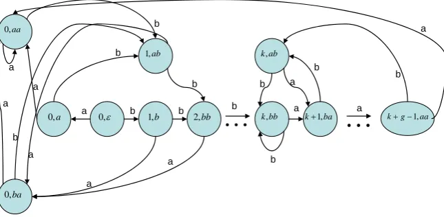
Taking the cross product of states of D with and then trimming inaccessible states, one obtains the second-order DFA with initial state
{
2, , ,a b aa ab ba bb, , ,
ε
≤
Σ =
}
( 2)
D
(0, )ε that is depicted in Fig. 2. The AMC
{ }
Yτ τT=2has states of the form ( , , , )q st φ Δ , whereare states of , and ( , ( , )q st ( 2)
D φ Δ) are incremented with visits to D( 2)’s final states. The value of φ
is incremented by 1 and Δ is incremented by k when state ( , is entered from ( 1 , indicating a k-run of . With each subsequent visit to one of the final states,
)
k bb
,
k− bb) b s'
Δ is
incremented by one. To compensate for counting visits to non-island states when the island is being left, g−1 is
subtracted from Δ on the transition from (k+ −g 1,aa) to (or from
(0,aa) (k+1,ba) to (0,aa) when g=2). For φ=1,…,ς+⎣⎢[T−ς(k+g)] /k⎥⎦ and Δ =1,…,T
( ⎢ ⎥⎣ ⎦x is the greatest integer less than or equal to x and
/( )
T k g
ς =⎢⎣ + ⎥⎦ ), let ψt( , , , )q st φ Δ =P Y[ t =( , , ,q st φ Δ)] . The backward variables are obtained as described earlier. The initial distribution and transition probabilities for the state sequence conditional on s o are, respectively,
2
0 2 2 2 2
0 2 2 2 ( ) ( , )
( )
( ) ( , )
S
s
s s
p s
s s
β β Ψ =
Ψ
∑
oo
o , (9)
1 1
1
1 1
( , , ) ( , )
( , )
( , ) t t t t S t t
t t
s s s
p s s
s
β
β
−−
− −
Ψ
= o o
o
o . (10)
We assume that k g, >2. To obtain
ψ
t recursively, begin with
2(0,aa, 0, 0) p aaS( )
ψ = o , ψ2(0,ba, 0, 0)= p baS( o) , 2(1,ab, 0, 0) p abS( )
ψ = o , ψ2(2,bb, 0, 0)=p bbS( o);
initial probabilities for other states are zero. For t=3,…,T ,
1
(0, , , ) (0, , , ) ( , )
t aa t ba p a ba
ψ φ Δ =ψ− φ Δ o
+ψt−1(k+ −g 1,aa, ,φ Δ + −g 1) (I Δ ≥k p a aa) ( ,o) +ψt−1(0,aa, , ) (φ Δ p a aa, )o ;
1
(0, , , ) (1, , , ) ( , )
t ba t ab p a ab
ψ φ Δ =ψ− φ Δ o
12 1( , , , ) ( , )
k t
j ψ j bbφ p a bb
− − =
+
∑
Δ o ;1
(1, , , ) (0, , , ) ( , )
t ab t aa p b aa
ψ φ Δ =ψ − φ Δ o
+ψt−1(0,ba, , ) (φ Δ p b ba, )o ;
1
(2, , , ) (1, , , ) ( , )
t bb t ab p b ab
ψ φ Δ =ψ− φ Δ o ;
1
( , , , ) ( 1, , , ) ( , )
t j bb t j bb p b bb
ψ φ Δ =ψ − − φ Δ o , j=3,…,k−1;
[
1]
( , , , ) ( 1, , 1, ) ( 1, )
t k bb t k bb k I k
ψ φ Δ = ψ− − φ− Δ − φ≥ Δ ≥
×p b bb o( , ) + ⎡⎣ψt−1( ,k bb, ,φ Δ −1) (p b bb, )o +ψt−1( ,k ab, ,φ Δ −1) (p b ab, )o ⎦⎤ Δ ≥ +I( k 1). ForΔ ≥ +k 1,
1
( , , , ) ( 1, , , 1) ( , )
t k ab t k ba p b ba
ψ φ Δ =ψ− + φ Δ − o
1 1
2 ( , , , 1) ( ,
g
t k aa p b aa
α ψ α φ
− − =
+
∑
+ Δ − o) ;0,aa
…
0,ba
0,a a 0,ε b 1,b
a a
2,bb
b
a
,
k bb
b
1,
k+ ba
,
k ab
a
b a
1,
k+ −g aa
…
b a
1,ab
a
b
b
a
b
a
b b
a
[image:6.595.138.461.59.217.2]b
Fig. 2. Second-order DFA D( 2) that recognizes words ending in an island
1
( 1, , , ) ( , , , 1) ( , )
t k ba t k bb p a bb
ψ + φ Δ =ψ− φ Δ − o
+ψt−1( ,k ab, ,φ Δ −1) (p a ab, )o ;
1
( 2, , , ) ( 1, , , 1) ( ,
t k aa t k ba p a ba
ψ + φ Δ =ψ− + φ Δ − o);
1
( , , , ) ( 1, , , 1) ( , )
t k aa t k aa p a aa
ψ +α φ Δ =ψ − + −α φ Δ − o ;
( 2< ≤ −α g 1).
The joint distribution of θ=( , )φ Δ is obtained by summing ( , , , )
t q st
ψ φ Δ over values of
(
q s, t)
.V.CONCLUSION
In [7], a method was introduced for computing distributions of statistics of state sequences of hidden Markov models. This paper extends the methodology to more general classes of hidden state sequences. It is shown that distributions can be computed in graphical models, both discriminative and generative, which have factors that depend on current and past states, but not future ones. Thus the results have very general applications. In future work, the authors will apply the methodology to analyzing real data.
REFERENCES
[1] L. R. Rabiner, “A tutorial on hidden Markov models and selected
applications in speech recognition, Proceedings of the IEEE, 77(2), 1989, pp. 257-289.
[2] J. D. Hamilton, “A new approach to the economic analysis of
non-stationary time series and the business cycle,” Econometrica, 57, 1989, pp. 357-384.
[3] A. Krogh, “Two methods for improving performance of a HMM and
their application for gene finding,” In T. Gaasterland, P. Karp, K. Karplus, C. Ouzounis, C. Sander, and A. Valencia, eds., Proceedings of the Fifth International Conference on Intelligent Systems for Molecular Biology, 1997, pp. 179-186, AAAI Press.
[4] R. Durbin, S. R. Eddy, A. Krogh, G. Mitchinson, Biological Sequence
Analysis: Probability Models of Proteins and Nucleic Acids.
Cambridge University Press, 1985, ch. 3.
[5] J. Blanchet, and M. Vignes, “Combined expression data with missing
values and gene interaction network analysis: a Markovian integrated
approach,” Proceedings of the 7th IEEE International Conference on
Bioinformatics and Bioengineering, 2007, pp. 366-373.
[6] M. A. Tingley and L. McLean, “Detection of patterns in noisy time
series,” The Canadian Journal of Statistics, 29(2), 2001, pp. 217-237.
[7] J. A. D. Aston and D. E. K. Martin, “Distributions associated with
general runs and patterns in hidden Markov models,” Annals of Applied Statistics, 1(2), 2007, pp. 585-611.
[8] J. Lafferty, A. McCallum, and F. Pereira, “Conditional random fields:
Probabilistic models for segmenting and labeling sequence data.
Proceedings of the ICML, 2001.
[9] C. Sutton, A. McCallum, and K. Rohanimanesh, “Dynamic conditional
random fields,” Journal of Machine Learning Research, 8, 2007, pp.
693-723.
[10] T. Dean and K. Kanazawa, “A model for reasoning about persistence
and causation,” Computational Intelligence, 5, 1995, pp. 142-150.
[11] J. C. Fu and M. V. Koutras, “Distribution theory of runs: A Markov
chain approach,” Journal of the American Statistical Association, 89, 1994, pp. 1050-1058.
[12] J. A. D. Aston and D. E. K. Martin, “Waiting time distributions of
competing patterns in higher-order Markovian sequences,” Journal of
Applied Probability, 42, 2005, pp. 977-988.
[13] D. E. K. Martin and J. A. D. Aston, “Waiting time distributions of
generalized later patterns,” Computational Statistics and Data
Analysis, 52(11), 2008, pp. 4879-4890.
[14] A. V. Aho and M. J. Corasick, “Efficient string matching: An aid to
bibliography search,” Communications of the ACM, 1975, 18(6), pp.
333-340.
[15] J. Hopcroft, “An algorithm for minimizing states in a finite
automaton,” in Proceedings of the International Symposium on the
Theory of Machines and Computations, 1971, pp. 189-196, Haifa, Israel.
log
n n
[16] M. E. Lladser, “Minimal Markov chain embeddings of pattern
problems,” Proceedings of the 2007 Information Theory and Applications Workshop. University of California, San Diego.
[17] S. Robin, F. Rodolphe, and S. Schbath, DNA, Words and Models:
Statistics of Exceptional Words. Cambridge University Press, 2005. [18] A. Bird, “CpG-rich islands as gene markers in the vertebrate nucleus,”
Trends in Genetics, 3, 1987,pp. 342-347.
[19] D. Takai and P. A. Jones, “Comprehensive analysis of CpG islands in
human chromosomes 21 and 22,” Proceedings of the National
Academy of Science USA, 2002, 99, pp. 3740-3745.
[20] Y. Wang and F. C. C. Leung, “An evaluation of new criteria for CpG
islands in the human genome as gene markers,” Bioinformatics, 20(7), 2004, pp. 1170-1177.
[21] S. V. N. Vishwanathun, N. N. Schraudolph, M. W. Schmidt, K. P.
Murphy, “Accelerated training of conditional random fields with stochastic gradient methods,” Proceedings of the 23rd International
Conference on Machine Learning, 2006, pp. 969-976.