IMSurReal: IMS at the Surface Realization Shared Task 2019

Proceedings of the 2nd Workshop on Multilingual Surface Realisation (MSR 2019), pages 50–58 50

IMSurReal: IMS at the Surface Realization Shared Task 2019

Xiang Yu, Agnieszka Falenska, Marina Haid, Ngoc Thang Vu, Jonas Kuhn Institut f¨ur Maschinelle Sprachverarbeitung

Universit¨at Stuttgart, Germany

firstname.lastname@ims.uni-stuttgart.de

Abstract

We introduce the IMS contribution to the Sur-face Realization Shared Task 2019. Our sub-mission achieves the state-of-the-art perfor-mance without using any external resources. The system takes a pipeline approach consist-ing of five steps: linearization, completion, in-flection, contraction, and detokenization. We compare the performance of our linearization algorithm with two external baselines and re-port results for each step in the pipeline. Fur-thermore, we perform detailed error analysis revealing correlation between word order free-dom and difficulty of the linearization task.

1 Introduction

This paper presents our submission to the Surface Realization Shared Task 2019 (Mille et al.,2019). We participate in both shallow and deep track of the shared task, where the shallow track requires the recovery of the linear order and inflection of a dependency tree, and the deep track additionally requires the completion of function words.

We approach both tasks with very similar pipelines, consisting of linearizing the unordered dependency trees, completing function words (for the deep track only), inflecting lemmata to word forms, and contracting several words as one token, and finally detokenizing to obtain the natural writ-ten text. We use machine learning models for the first four steps and a rule-based off-the-shelf deto-kenizer for the final step.

In the evaluation on the tokenized text, our sys-tem achieves the highest BLEU scores for each in-dividual treebank in both tracks, with an average of 79.97 for the shallow track and 51.41 for the deep track. In the human evaluation on four lan-guages, we also rank the first in terms of readabil-ity and adequacy.

2 Surface Realization System

Our system takes a pipeline approach, which consists of up to five steps to produce the fi-nal detokenized text. The steps are: lineariza-tion (§2.2), completion (§2.3), inflection (§2.4), contraction (§2.5), and detokenization (§2.6), among which completion is used only in the deep track. All the steps except for the rule-based deto-kenization use the same Tree-LSTM encoder ar-chitecture (§2.1). As the multi-task style training hurt performance in the preliminary experiments, all the steps are trained separately.

Since the submission is mostly based on our system described in Yu et al. (2019b), here we mainly focus on the changes introduced for this shared task, and we refer the reader to Yu et al. (2019b) for more details, especially on the ex-planation and ablation experiments of the Tree-LSTM encoder and the linearization decoder.

2.1 Tree-LSTM Encoder

Representation of each token in the tree is based on its lemma, UPOS, morphological features, and dependency label. We use embeddings for the lemma, UPOS and dependency label, and employ an LSTM to process the list of morphological fea-tures.1 We then concatenate all of the obtained vectors as the representation of each token (v◦).

The representation is further processed by a bidirectional Tree-LSTM to encode the tree struc-ture information. The encoder is generally the same as described inYu et al.(2019b), consisting of two passes of information: a bottom-up pass followed by a top-down pass. In the bottom-up pass, we use a Tree-LSTM (Zhou et al.,2016) to compose the bottom-up vector of the head from the vectors of the dependents, attended by the

1_{There could be better treatment of the morphological}

token-level vector of the head, denoted asv↑. The bottom-up vectors are then fed into a sequential LSTM for the top-down pass from the root to each leaf token, so that every token has access to all the descendants of all its ancestors, namely all tokens in the tree. The output vector is denoted asv↓.

For linearization, we use the concatenation of

v↑andv↓as the representation of each token. For the other tasks, where the sequence is already de-termined, we additionally use a sequential bidi-rectional LSTM to encode the sequence, with the tree-based vectors as input.

2.2 Linearization

The linearization algorithm is the same as in Yu et al. (2019b), which is in turn based on the lin-earizer described by Bohnet et al. (2010). The algorithm takes an divide-and-conquer strategy, which orders each subtree (a head and its depen-dents) individually, and then combines them into a fully linearized tree.2

The main improvement of our algorithm to Bohnet et al.(2010) is that instead of ordering the subtrees from left to right, we start from the head (thus called the head-first decoder), and add the dependents on both sides of the head incremen-tally. We also train a left-to-right and a right-to-left decoders to form an ensemble with a shared encoder, which is shown in Yu et al. (2019b) to achieve the best performance.

We use beam search to find the best lineariza-tion order of each subtree, where the best N par-tial hypotheses are kept to expand at each step. For the head-first decoder, we use two LSTMs to track the left and right expansion of the sequence (only one LSTM is needed for the left-to-right or right-to-left expansion), and the score of the se-quence is calculated from the concatenation of the two LSTM states followed by an MLP.

Note that in the shared task some tokens are provided with information about the relative word order to its head.3 We use these constraints in our decoder so that the hypotheses violating the constraints are ignored. Preliminary experiments

2_{This algorithm can only create projective trees. An}

method to bypass the projective constraints is described in

Bohnet et al.(2012). However, we did not use this method

and only produce projective trees due to limited time.

3_{The information are encoded in the morphological}

fea-tures, such aslin=+2, which means this token must appear after the token with the featurelin=+1after the head. They are provided for the cases that do not have a unique correct order, e.g., punctuation or coordinating conjunction.

showed that disregarding this word order informa-tion would decrease the BLEU score by 2-3 points.

2.3 Completion

The completion model for the deep track takes the output of the linearization model as input and in-sert function words into the linearized subtrees.

Similarly to the linearization algorithm, we also use a head-first strategy to complete each subtree. We use two pairs of LSTMs to encode the se-quence: a pair of forward and backward LSTMs for the left dependents, and a pair for the right de-pendents, where “forward” means from the head to the end and “backward” means from the end towards the head. Since the two pairs are symmet-rical, we only describe the decoding process to the right side of the head.

We use a pointer to indicate the current to-ken, which initially points to the head. We use the backward LSTM to encode the upcoming sequence of linearized tokens, and the forward LSTM to encode the already processed tokens up to the pointer (which includes both the previously linearized tokens and the newly generated tokens). At each decoding step, we concatenate the for-ward LSTM output of the current pointed token and the backward LSTM output of the next token, and calculate a softmax distribution of all possible function words, as well as a special symbol ⇒, which moves the pointer to the next token. If a new token is generated, the pointer will point to the new token. If⇒ is predicted and the pointer al-ready reached the last token in the sequence, then the completion process is terminated.

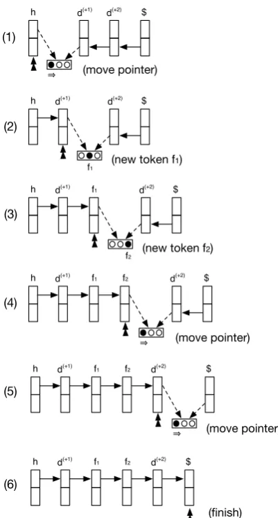
Figure1illustrate an example of the completion process to the right side of the head, where the lin-earized tokens are [h, d(+1), d(+2), $], h is the head, d(+1) and d(+2) are right dependents, and $ indi-cates the end of the subtree. In step (1) the sym-bol⇒is predicted, therefore we move the pointer from the h to d(+1); in step (2) a new token f1 is

created and attached to d(+1); in step (3) another token f2is created and attached to f1; in step (4) the

pointer is moved to d(+2); in step (5) the pointer is moved again to $, which terminates the process and outputs the sequence [h, d(+1), f1, f2, d(+2)].

prelimi-h $

h $

d(+1) _d(+2)

d(+1)

d(+2)

f1

h d(+1) $

d(+2)

f2

f1

h d(+1) $

d(+2)

f1 f2

h d(+1) $

d(+2)

f1 f2 (move pointer)

(1)

(2)

(3)

(4)

(5)

(new token f1)

(new token f2)

(move pointer)

(move pointer)

h d(+1) $

d(+2)

f1 f2

(6)

(finish)

Figure 1: An example of the completion process to the right side, where the right arrows illustrate the forward LSTM, and the left arrows the backward LSTM.

nary experiments, including joint linearization and completion, interleaving the left and right comple-tion processes, and beam-search for complecomple-tion. All approaches yielded lower performance than the described method.4 However, we note that the completion step seems to have the most po-tential to benefit from external language models. We observe that many generated function words are syntactically correct but semantically implau-sible, and the language models are generally good at capturing semantic coherence. We plan to in-corporate language models in the future work.

4_{Admittedly, most of the experiments are rather brief,}

more careful design and thorough experiments might lead to different results.

2.4 Inflection

The inflection model is the same as in Yu et al. (2019b). It generates a sequence of edit opera-tions that modifies the lemma into the inflected word form. The model takes the characters in the lemma as input and encodes through a bidi-rectional LSTM. A binary feature is concatenated to the vector of each character which functions as a pointer to indicate the input character currently to be processed. At each step, the decoder attends to the input vectors and predicts an output, which could be a symbol 3 to copy the current input character, a symbol 7 to ignore the current input character, or a character from the alphabet to gen-erate a new one. When3 or7 is predicted, the input pointer will move one step forward, while if a character is generated, the input pointer does not move.

The ground truth of such sequence is calculated from the Levenshtein edit operations between the lemma and the word form, where only insertion and deletion is allowed (no substitution).

Our model is in a way similar to the hard mono-tonic attention in Aharoni and Goldberg (2017), but we use a much simpler source-target align-ment (Levenshtein edit operations), and we use copy as an edit operation to avoid completion er-rors while they do not. Furthermore, our edit operations are associated with the moving of the pointer, while they treat moving the pointer as an atomic operation, which lead to longer prediction sequences. Generally, our model performs on a par with theirs, see the comparison in Yu et al. (2019b).

2.5 Contraction

In Yu et al. (2019b) we described a rule-based contraction method by constructing an automa-ton from the training data, which works reason-ably well for most of the languages where the contraction is trivial. However, it works rather poorly for Arabic since the contraction is not just among closed class function words but also con-tent words, so that the coverage of the rules is very small. It is also problematic for the verb-pronoun contraction in Spanish and Portuguese although they are much less frequent.

that need to be contracted. Then it concatenates the group as a character sequence and predicts the contracted word form as output. We use a simple Seq2Seq model for the contraction due to limited time, although an edit based model similar to the one for inflection might yield better results.

2.6 Detokenization

The detokenization step is the same as described in Yu et al. (2019b), namely a rule-based tool MosesDetokenizer.5After the submission we real-ized that the tool removes all empty spaces in Ko-rean texts, similar to Chinese and Japanese. How-ever, Korean actually uses empty spaces to sepa-rate words, thus we expect lower score in the hu-man evaluation for this language.

2.7 Discussion on Pipeline Order

In our pipeline, we choose the order of lineariza-tion, complelineariza-tion, and finally inflection. Our ratio-nale for such order is as follows: (1) the inflec-tion in some cases depends on the linearized se-quence of lemmata, e.g., the English determiner “a/an” depends on whether the following noun be-gins with an vowel, therefore inflection is the last of the three steps; (2) the search-based lineariza-tion model is more reliable than the greedy com-pletion model, therefore we first perform lineariza-tion to reduce error propagalineariza-tion.

However, this choice is only based on our intu-ition, and one could come up with arguments for the alternative orders. For example, since inflec-tion is the easiest and most accurate task, perform-ing it first might further reduce error propagation. Further experiments are needed to determine the best order in the pipeline. Alternatively, a care-fully designed joint prediction might address the error propagation problem, however, our initial at-tempts did not yield positive outcome.

2.8 Implementation Details

All the neural models are implemented with the DyNet library(Neubig et al., 2017), and the full system is available at the first author’s website.6 We use the embedding size of 64 for lemma and character, and 32 for UPOS, XPOS, morpholog-ical features, and dependency labels. The output dimension of the bottom-up and top-down encoder

5_{https://pypi.org/project/}

mosestokenizer/

6_{https://www.ims.uni-stuttgart.de/}

institut/mitarbeiter/xiangyu/

LSTMs, as well as all the decoder LSTMs, are equal to the input dimension. The beam size for the linearization is 32. We train the model up to 100000 steps without batching using the Adam op-timizer (Kingma and Ba,2014), test on the devel-opment set every 2000 steps, and stop training if there is no improvement 10 times in a row. All the hyperparameters are only minimally tuned to bal-ance speed and performbal-ance, and kept the same for all languages.

The training and prediction of each treebank are run on single CPU cores. Depending on the treebank size, the training time of linearization models typically ranges from 1 to 10 hours. The completion, inflection, and contraction models are much faster, mostly under 1 hour, since they are all greedy models.

The prediction speed is around 10 sentence per second, which is not very fast, however, we did not perform any optimization toward speed (e.g. mini-batch, multi-processing, etc.) due to the ex-perimental nature of our work.

3 Data

The training and test data in the shared task is based on Universal Dependencies (Nivre et al., 2016), see the overview paper for the details.

We do not use any external resources for our system, except that we concatenate the training treebanks for some languages (see Table 3 and 4). However, not all treebanks benefits from the concatenation, since the idiosyncrasies in the UD treebanks can hurt the performance as noted in Bj¨orkelund et al.(2017), where the concatenation of multiple UD treebanks also hurts parsing per-formance.

Evaluation in the shared task is also performed on out-of-domain datasets, namely the automati-cally parsed trees from some in-domain treebanks and the unseen PUD treebanks. We use the same model for the automatically parsed trees as for the gold ones, and use the model trained on concate-nated treebanks for the PUD test data.

the submission, we only choose to decompose the XPOS for Korean because it can be easily split by the “+” delimiter and both Korean treebanks do not have morphological features otherwise. We also use the real stems in the Korean treebanks by removing the suffixes after the “+” delimiter in the lemmata, in order to reduce the out-of-vocabulary problem, and the information on the suffixes are well preserved in the morphological features de-rived from the XPOS.

Finally, since contraction appears only in Ara-bic, Spanish, French and Portuguese, we therefore only train contraction models for these languages.

4 Evaluation

The automatic evaluation results of our submis-sion to the shared task are shown in Table 1 and Table 2 for the shallow and deep tracks, respec-tively. The first three columns contain the BLEU, DIST, and NIST scores of our system, and the fourth column is the difference of BLEU scores between our system and the best system among other participants for each treebank.

Our system achieve the best performance for all treebanks in both tracks. Comparing to the best scores of other teams, the differences range from single digits for the English treebanks to about 20 points for most other treebanks and 38 points for Arabic. In the out-of-domain scenario, our system performs very stable in most of the cases. How-ever, comparing to the English and Japanese PUD treebanks, the performance drop on Russian PUD treebank is quite notable. Our conjecture is that the annotation of the PUD treebank is much closer to the GSD treebank than the SynTagRus treebank. Since we use both treebanks for training, the much larger size of SynTagRus might have dominated the training.

In the human evaluation (seeMille et al.(2019) for details), we also rank the first in all four lan-guages (English, Russian, Chinese and Spanish) both for readability and adequacy.

5 Analysis

5.1 Pipeline Performance

Table 3 and 4 show the results on the develop-ment sets of the in-domain treebanks for the shal-low track and deep track, respectively. We also provide the linearization baselines byPuduppully

BLEU NIST DIST ∆BLEU

ar padt 64.90 12.22 73.71 38.50 en ewt 82.98 13.61 86.72 3.29 en gum 83.84 12.69 83.49 1.45 en lines 81.00 12.71 82.21 5.51 en partut 87.25 11.01 85.68 8.27 es ancora 83.70 14.69 79.82 7.23 es gsd 82.98 12.77 79.45 12.83 fr gsd 84.00 12.45 84.15 23.85 fr partut 83.38 10.36 82.32 17.37 fr sequoia 85.01 12.53 85.13 22.22 hi hdtb 80.56 13.07 79.07 11.33 id gsd 85.34 12.83 83.92 21.63 ja gsd 87.69 12.42 87.17 24.10 ko gsd 74.19 12.27 80.95 28.11 ko kaist 73.93 13.00 78.69 26.70 pt bosque 77.75 12.15 79.80 25.06 pt gsd 75.93 13.07 79.33 23.43 ru gsd 71.23 12.15 73.04 16.14 ru syntagrus 76.95 15.08 78.66 16.96 zh gsd 83.85 12.78 83.18 15.31 en pud 86.61 13.47 87.00 2.54 ja pud 86.64 13.02 84.04 20.12 ru pud 58.38 10.91 77.12 6.01 en ewt-pred 81.80 13.46 85.35 4.59 en pud-pred 82.60 13.26 86.18 1.94 es ancora-pred 83.31 14.61 81.14 6.03 hi hdtb-pred 80.19 13.05 78.88 10.27 ko kaist-pred 74.27 13.02 79.12 27.55 pt bosque-pred 78.97 12.14 81.56 25.33 AVG 79.97 12.79 81.62 15.64

Table 1: Automatic Evaluation Results of the shallow track (T1) and the BLEU difference with the best sys-tem among other participants for each treebank.

BLEU NIST DIST ∆BLEU

en ewt 54.75 11.79 76.30 25.17 en gum 52.45 11.04 73.07 25.85 en lines 47.29 10.63 71.93 18.21 en partut 45.89 9.03 67.45 17.04 es ancora 53.13 12.38 68.58 16.15 es gsd 51.17 10.82 68.85 16.52 fr gsd 53.62 10.79 68.82 28.02 fr partut 46.95 8.27 68.99 18.76 fr sequoia 57.41 11.00 72.06 28.85 en pud 51.01 11.45 72.31 24.45 en ewt-pred 53.54 11.55 74.99 24.91 en pud-pred 47.60 11.08 71.65 21.83 es ancora-pred 53.54 12.36 70.02 16.13 AVG 51.41 10.94 71.16 21.68

P16 B10 lin∗ lin inf con final ar padt 77.73 82.69 84.24 87.27 95.63 91.59 68.58 en ewt 79.10 82.71 85.11 88.01 98.47 84.50 en gum 74.03 82.36 83.69 87.29 98.23 84.35 en lines(+) 69.47 75.69 78.39 82.40 97.86 79.05 en partut 71.45 80.11 86.38 89.14 97.94 86.25 es ancora 74.57 81.61 83.47 85.33 99.51 99.86 84.43 es gsd(+) 78.28 82.32 83.53 86.18 99.18 99.09 84.04 fr gsd(+) 82.99 85.26 87.02 89.74 98.63 99.47 86.98 fr partut 71.46 83.92 87.07 90.08 96.95 99.44 84.17 fr sequoia 74.16 83.66 87.09 90.39 98.20 99.58 86.51 hi hdtb 79.83 82.03 82.79 85.25 98.11 81.62 id gsd 74.68 78.27 81.23 86.05 99.51 84.62 ja gsd 86.20 89.08 90.41 92.55 98.69 89.49 ko gsd(+) 67.55 69.48 76.05 79.66 96.74 74.25 ko kaist(+) 76.98 77.47 78.73 80.01 97.32 76.04 pt bosque 76.97 80.30 82.48 84.35 99.31 98.23 80.75 pt gsd 83.19 86.53 87.17 89.24 94.99 99.84 76.89 ru gsd 68.32 74.04 74.64 79.09 95.98 73.66 ru syntagrus(+) 73.58 77.01 78.52 80.97 97.84 76.28 zh gsd 68.92 75.60 81.22 84.10 100.00 83.34 AVG 75.47 80.51 82.96 85.86 97.95 81.29

Table 3: Development results in the shallow track, including the linearization baselines.

lin comp inf con final en ewt 80.17 67.70 97.98 55.27 en gum(+) 76.14 61.44 97.72 50.53 en lines(+) 76.63 60.47 97.16 47.17 en partut(+) 73.80 60.63 97.63 44.59 es ancora 77.88 66.95 98.25 99.85 53.57 es gsd 77.98 69.72 97.85 99.71 53.81 fr gsd(+) 81.36 73.20 97.63 99.26 57.46 fr partut(+) 75.36 65.94 94.64 98.39 48.17 fr sequoia(+) 80.03 73.01 97.04 99.60 58.27 AVG 77.40 66.42 97.24 51.70

Table 4: Development results in the deep track.

et al.(2016) (P16) andBohnet et al.(2010) (B10).7 The columns show different evaluation metrics on different targets. Except for the final column, each one evaluates on only one step assuming all previ-ous steps are gold.

In Table3, columns 1-4 are the BLEU scores of linearization evaluated on the lemmata, column 5 is the accuracy of inflection, column 6 is BLEU score on the contracted word form (empty cells means contraction is not applied), column 7 is the final BLEU score of the full pipeline. The col-umn lin* shows the models trained on single tree-banks and without using the word order informa-tion, which allows a fair comparison to the two baselines. The models marked with + are trained with concatenated treebanks for the submission,

7_{We run the two baseline systemsas is, where we only}

convert the input format to ensure all systems are using the same information and keep their default options.

which performs slightly better than the single tree-bank, typically by 0.5-1 BLEU points. For each treebank, we either use the concatenated treebank to train all steps in the pipeline or use the sin-gle treebank for all steps, depending on the final BLEU score on the development set.

In Table4, column 1 is the BLEU score on the lemmata of the given content words, columns 2 is the BLEU score on the lemmata including gen-erated tokens, column 3 is the accuracy on word forms, column 4 is the BLEU score of contracted word forms, and column 5 is the BLEU score of the full pipeline. Similar to Table 3, the models marked with + are trained with concatenated tree-banks.

In the shallow track, our linearization model outperforms the best baseline (Bohnet et al.,2010) by 2.5 BLEU points on average. The inclusion of word order information (and treebank concatena-tion to a much smaller extent) brings about 3 addi-tional points. For the deep track, the BLEU score of linearization is much higher than completion, which motivates our decision to perform lineariza-tion before complelineariza-tion.

5.2 Word Order Preferences

In this section we analyze the relation between word order preferences of each language and the errors made by the linearizer,8 characterized by

8_{Note that an “error” is counted when the predicted order}

0.00 0.05 0.10 0.15 0.20 0.25 0.30 0.35 0.40 Freadom of head direction

0 1 2 3 4 5 6 7

% errors

ru_gs ru_sy

ar hi

id

ja

zh Slavic

Korean Germanicother Romance

(a) Head direction freedom vs. errors.

0.0 0.1 0.2 0.3 0.4 0.5 0.6 Freadom of sibling ordering 0.0

2.5 5.0 7.5 10.0 12.5 15.0

% errors

ar hi id

ja zh

Slavic

Korean Germanicother Romance

(b) Sibling ordering freedom vs. errors.

Figure 2: The correlation of word order freedom and linearization errors. Different language families are marked with different colors.

case nmod det nsubj amod obl obj advmod conj cc

ar_padt en_ewt en_gum en_lines en_partut es_ancora es_gsd fr_gsd fr_partut fr_sequoia hi_hdtb id_gsd ja_gsd ko_gsd ko_kaist pt_bosque pt_gsd ru_gsd ru_syntagrus zh_gsd

x

x

0.0 0.2 0.4 0.6 0.8

Freedom of head direction

(a) Head direction freedom of each dependency re-lations in each training set.

case nmod det nsubj amod obl obj advmod conj cc

ar_padt en_ewt en_gum en_lines en_partut es_ancora es_gsd fr_gsd fr_partut fr_sequoia hi_hdtb id_gsd ja_gsd ko_gsd ko_kaist pt_bosque pt_gsd ru_gsd ru_syntagrus zh_gsd

x

x

0.0 2.5 5.0 7.5 10.0 12.5 15.0 17.5

% errors

(b) Head direction errors of each dependency rela-tions in each development set.

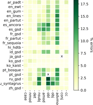
Figure 3: Detailed visualization of head direction freedom vs. linearization errors of the 10 most frequent depen-dency relations in each treebank, where “x” means no such relation in the treebank.

two types of word order preferences as defined in Yu et al.(2019a):

head direction– whether the dependent appears to the left or the right side of the head;

sibling order– the order of a pair of dependents on the same side of the head.

We then define the freedom of these two types of word order preferences, namely the entropy of the word order of each dependency relation, which is described in details inYu et al.(2019a)9. In both

this does not mean that the predicted one is incorrect. The variation of word order in natural languages can not be triv-ially evaluated by the single reference BLEU score, human judgement is thus needed for a more accurate evaluation.

9_{Here we only use the dependency relations to}

character-ize the word orders for simplicity of visualization, whileYu

et al.(2019a) additionally use the UPOS tag, which is more

types of word orders, higher freedom means less constraints on the word order.

We also calculate the error rate of the linearizer by the dependency relations:

head direction– whether the dependent appears on the correct side of the head;

sibling order – whether a pair of dependents on the same side of the head has the correct order.

Figure2 shows the correlation of freedom and linearization errors of the two types of word or-ders. For both head direction (Figure2a) and sib-ling ordering (Figure 2b), we can observe quite strong correlation of the freedom and linearization errors. For the head direction, both Russian tree-banks have the highest freedom, and the linearizer

case nmod det nsubj amod obl obj advmod conj cc

ar_padt en_ewt en_gum en_lines en_partut es_ancora es_gsd fr_gsd fr_partut fr_sequoia hi_hdtb id_gsd ja_gsd ko_gsd ko_kaist pt_bosque pt_gsd ru_gsd ru_syntagrus zh_gsd

x

x

0.0 0.1 0.2 0.3 0.4 0.5 0.6 0.7 0.8

Freedom of sibling ordering

(a) Sibling ordering freedom of each dependency relations in each training set.

case nmod det nsubj amod obl obj advmod conj cc

ar_padt en_ewt en_gum en_lines en_partut es_ancora es_gsd fr_gsd fr_partut fr_sequoia hi_hdtb id_gsd ja_gsd ko_gsd ko_kaist pt_bosque pt_gsd ru_gsd ru_syntagrus zh_gsd

x

x

0 5 10 15 20 25

% errors

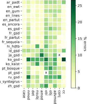
(b) Sibling ordering errors of each dependency re-lations in each development set.

Figure 4: Detailed visualization of sibling ordering freedom vs. linearization errors of the 10 most frequent dependency relations in each treebank, where “x” means no such relation in the treebank.

also makes the most errors. Verb final languages such as Korean, Japanese and Hindi, on the con-trary, have the lowest freedom and the least errors. For the sibling ordering, both Korean treebanks have the highest freedom and linearization error rate. However, there are no treebanks with very low freedom or error rate, which suggests that the ordering of arguments are generally less strict than the head direction in all languages.

We then look into the errors of our system in more details. We take ten most common depen-dency relations in all the treebanks (we map the language-specific relation subtypes to their gen-eral type, e.g., nmod:poss is mapped to nmod) and calculate their freedom and the linearization error rate. Figure3 presents results for the head direction constraint, where the intensity patterns of the freedom and error rate align very well. In-terestingly, the verb-final languages have very low freedom and error rate across almost all relations, not only verb arguments. For the most other lan-guages, obl and advmod are difficult; amod is dif-ficult for Romance languages; and nsubj is diffi-cult for Russian.

Figure 4 shows the freedom and error rate for sibling ordering. The freedom of particular re-lations (Figure 4a) and their linearization errors (Figure 4b) also show quite similar patterns, al-though less clear than the head direction.

In particular, some relations with very high

free-dom do not have high error rate, e.g. many verb arguments in Japanese. This suggests that the lex-icalized linearization model can capture more so-phisticated word order information than the coarse word order preferences defined by the dependency relations.

6 Conclusion

We have presented our surface realization system, which performs both shallow and deep comple-tion. The system achieves state-of-the-art results without any external data.

As future work, we plan to focus on improving the completion model, since it is currently the per-formance bottleneck of the deep generation task, which is a more realistic task for NLG applica-tions. We also plan to incorporate ranking meth-ods with and without external language models to further improve the linearization, since the de-scribed results suggest that there is room for im-provement.

Acknowledgements

References

Roee Aharoni and Yoav Goldberg. 2017.

Morpholog-ical Inflection Generation with Hard Monotonic At-tention. In Proceedings of the 55th Annual Meet-ing of the Association for Computational LMeet-inguistics (Volume 1: Long Papers), pages 2004–2015.

Anders Bj¨orkelund, Agnieszka Falenska, Xiang Yu,

and Jonas Kuhn. 2017. IMS at the CoNLL 2017

UD Shared Task: CRFs and Perceptrons Meet Neu-ral Networks. InProceedings of the CoNLL 2017 Shared Task: Multilingual Parsing from Raw Text to Universal Dependencies, pages 40–51, Vancouver, Canada. Association for Computational Linguistics.

Bernd Bohnet, Anders Bj¨orkelund, Jonas Kuhn,

Wolf-gang Seeker, and Sina Zarrieß. 2012. Generating

Non-Projective Word Order in Statistical Lineariza-tion. In Proceedings of the 2012 Joint Confer-ence on Empirical Methods in Natural Language Processing and Computational Natural Language Learning, pages 928–939.

Bernd Bohnet, Leo Wanner, Simon Mille, and

Ali-cia Burga. 2010. Broad Coverage Multilingual

Deep Sentence Generation with a Stochastic Multi-Level Realizer. In Proceedings of the 23rd Inter-national Conference on Computational Linguistics, pages 98–106. Association for Computational Lin-guistics.

Diederik P. Kingma and Jimmy Ba. 2014. Adam: A

Method for Stochastic Optimization.

Simon Mille, Anja Belz, Bernd Bohnet, Yvette

Gra-ham, and Leo Wanner. 2019. The Second

Mul-tilingual Surface Realisation Shared Task (SR’19):

Overview and Evaluation Results. InProceedings of

the 2nd Workshop on Multilingual Surface Realisa-tion (MSR), 2019 Conference on Empirical Methods in Natural Language Processing (EMNLP), Hong Kong, China.

Graham Neubig, Chris Dyer, Yoav Goldberg, Austin Matthews, Waleed Ammar, Antonios Anastasopou-los, Miguel Ballesteros, David Chiang, Daniel

Clothiaux, Trevor Cohn, et al. 2017. Dynet: The

Dynamic Neural Network Toolkit. arXiv preprint arXiv:1701.03980.

Joakim Nivre, Marie-Catherine De Marneffe, Filip Ginter, Yoav Goldberg, Jan Hajic, Christopher D Manning, Ryan McDonald, Slav Petrov, Sampo

Pyysalo, Natalia Silveira, et al. 2016. Universal

De-pendencies v1: A Multilingual Treebank Collection. In Proceedings of the Tenth International Confer-ence on Language Resources and Evaluation (LREC 2016), pages 1659–1666.

Ratish Puduppully, Yue Zhang, and Manish

Shrivas-tava. 2016. Transition-based Syntactic

Lineariza-tion with Lookahead Features. InProceedings of the 2016 Conference of the North American Chapter of the Association for Computational Linguistics: Hu-man Language Technologies, pages 488–493.

Xiang Yu, Agnieszka Falenska, and Jonas Kuhn.

2019a. Dependency Length Minimization vs. Word

Order Constraints: An Empirical Study On 55 Treebanks. In Proceedings of the First Workshop on Quantitative Syntax (Quasy, SyntaxFest 2019), pages 89–97, Paris, France. Association for Com-putational Linguistics.

Xiang Yu, Agnieszka Falenska, Ngoc Thang Vu, and

Jonas Kuhn. 2019b. Head-first linearization with

tree-structured representation. InProceedings of the

12th International Conference on Natural Language Generation, Tokyo, Japan.

Yao Zhou, Cong Liu, and Yan Pan. 2016.