Labour market rents and Irish industrial policy

363

Paper presented at the Annual Conference of the Irish Economic Association.

*I am grateful to Joe Durkan and Eric Strobl for advice on the Data and Paul Sheridan of the Central Statistics Office for a spreadsheet of the Input-Output Tables, Frank Barry and anonymous referees. All errors are mine.

Labour Market Rents and Irish Industrial Policy

FRANK WALSH*

University College Dublin

Abstract: This paper examines the issue of whether harmonising taxes across the traded and non-traded sectors is desirable. Preferential treatment for the non-traded sector might be justified if either the output response of subsidies are higher in the traded sector or if the jobs generated in the traded sector are “better” than those in the non-traded sector. I examine these two issues using a simple two sector small open economy model to analyse the first question and input-output analysis to analyse the second. I conclude that there is no compelling argument for lower taxes on the traded sector.

I INTRODUCTION

questions. First, will subsidising the traded sector (or having preferential tax treatment for the traded sector) increase output? Second, are jobs created as a result of a subsidy to the traded sector more “desirable” than jobs created as a result of a subsidy to the non-traded sector? The first issue has been analysed in O’Rourke (1994) and Denny, Hannan and O’Rourke (1995) who use a computable general equilibrium model to assess the impact of a subsidy on equilibrium output and employment in other sectors while NESC (1990) emphasises the role of industrial policy in tackling unemployment. Denny, Hannan and O’Rourke (1995) predict that harmonising capital taxes will increase unemployment. As they point out, this conclusion depends on the assumption of greater capital mobility in the modern sector. It could be argued that this is a short-run result in that in the long-run capital would be equally mobile across sectors. I develop a two sector small open economy model to examine under what circumstances the output response of a subsidy to the traded sector would be greater than the output response in the non-traded sector and conclude that there is not a compelling argument that output will increase more in the traded sector.

Another possibility is that the response to a subsidy in the traded sector will be greater because traded sector jobs are more productive than non-traded jobs as discussed below. To address the second issue of whether subsidising the traded sector creates more “desirable” jobs than subsidising the non-traded sector I use a framework developed by Dickens (1995) which allows us to measure the returns in wages and employment from subsidising particular sectors where there are twenty-eight sectors. Dickens’s analysis is based on models outlined in Katz and Summers (1989) or Bulow and Summers (1986). In these models workers earn high rents in particular sectors. This justifies an industrial policy favouring these sectors. McKeon (1980) states that “The IDA’s experience to date is that the labour employed in projects provides the greatest single contribution to discounted value added”; so looking at industrial policy as a way of generating employment rents seems reasonable.

While the analysis was hampered by poor wage data in particular some of the empirical results were surprising. Some of the service sectors had the highest measured rents. In particular when we account for the fact that gross wage differentials overstate rents and that many workers in jobs resulting from subsidies come from sectors where they had previously been earning rents, the results do not support subsidising the manufacturing sector.

cannot be used to evaluate the argument for subsidising particular sectors since it looks at the degree to which manufacturing jobs support service sector jobs, but not the other way around. If, for example, particular service sectors make significant purchases from domestic industry, it could be that it is the services sector that should be subsidised or that there is no strong argument for subsidising one sector over another.

II A SIMPLE MACRO MODEL

One justification for subsidising the traded over the non-traded sector is that it may generate a bigger output response because the size of the non-traded sector is limited (see the comments by Kieran Kennedy in the discussion following O’Rourke (1994) for example). It could be that a pound’s worth of subsidy generates more output in the traded compared to the non-traded sector.1 _{In this} section I analyse the issue of what determines the output response from a pound’s worth of subsidy given either to the traded or the non-traded sector. The price in the traded sector is determined on the world market and is exogenous. The price in the non-traded sector is determined by the intersection of domestic supply and demand. Since factors can move freely between the two sectors, I will assume both sectors face the same supply elasticity. Figure 1 illustrates the effect of subsidising output in the traded sector. The supply curve shifts to the right, output increases but the price remains unchanged. If non-traded goods are used in traded production, the higher quantity of tradeables will lead to an increase in demand for tradeables and a higher price and quantity. If non-tradeables are used in tradeable production the higher price for non-non-tradeables will shift the supply curve for tradeables inwards. We might expect equilibrium output in both sectors to increase if the traded sector is subsidised.

Figure 2 analysis a subsidy to the non-traded sector. The non-traded supply curve shifts down leading to a lower price. If non-tradeables are an input in tradeable production the supply for tradeables increases and the higher traded output increases demand for non-tradeables.

The next step is to derive a condition that will determine whether a pound’s worth of subsidy will generate more income overall if it is spent in the traded or non-traded sector. This will depend on the relative size of the sectors and the output responses outlined graphically above. I then use a two sector constant elasticities model to derive a sufficient condition for when it will be cheaper to subsidise the non-traded sector. The cost per unit of output of a percentage subsidy of Tj on output in the traded and non-traded sectors are given respectively

in Equations (1) and (2). Pj is the price level in the traded (t) sector and the starting price in the non-traded (n) sector. A subsidy in sector j causes growth π jn in the non-traded price level (traded prices are exogenous). Qj is initial output in sector j, g_j is the percentage growth in output in sector j from a subsidy on sector j and gjk is the percentage growth in output in sector j from a change in the subsidy rate in sector k. The numerators in the two equations below are the costs of an ad valorem subsidy Tj on each sector at the post subsidy prices. The denominators are the value of all output produced as a result of the subsidy evaluated at the post subsidy prices.

T_tP_tQ_t(1+g_t)

P_tQ_tg_t+P_n(1+ Π_nt)Q_ng_nt (1) Figure 1: Subsidising the Traded Sector

T_nP_nQ_n(1+g_n)(1+ Π_nn)

P_nQ_ng_n(1+ Πn_n)+P_tQ_tg_tn (2)

We call traded share of income z=PtQt/(PtQt+PnQn) and non-traded share (1–z), Equations (1) and (2) can be rewritten:

T_t(1+g_t) g_t+ 1−z

z 

 (1+ Πnt)gnt

=Tt(1+gt)

g_t+X (1’)

T_n(1+g_n)

g_n+ z 1−z   

1 1+ Π_nn  

 gtn

= Tn(1+gn)

g_n+Y (2’)

Equation (1’) shows the cost of a subsidy on the traded sector per pounds worth of output generated and (2’) the cost of a subsidy on the non-traded sector per pounds worth of output generated. We can see from (1’) and (2’) that if gn>gt and Y>X<1 these are sufficient conditions for the cost of generating output by subsidising the traded sector to be more expensive than subsidising the non-traded sector. The next step is to look at a simple structure for the economy to try and shed some light on when these sufficient conditions will hold.

I assume a competitive two sector economy with constant-elasticity demand and supply curves except for the demand for tradeables which is infinite at the world price.

Qns =An[Pn(1+Tn)]εs (3)

Qt s₌

A_t[P_t(1+T_t)]εs_P

n

εtn ₍₄₎

Qnd =BnPn εd_Q

t

εnt ₍₅₎

than subsidising traded output, incorporating the increase in demand for non-tradeables resulting from this income increase would magnify the result by increasing income further.

We can solve for the non-traded price by setting supply equal to demand in each sector:

P_n =e

εsln 1₁+_T n



  + εntln(pt+ptTt)εs+ εntln At± ln An_B n



 

εs− εd− εntεtn

(6)

Using this expression for non-tradeable prices in Equations (3) and (4) gives us reduced form equations for tradeable and non-tradeable equilibrium output. To get the percentage change in output in each sector we take the derivative of the log of output in each sector with respect to a change in the tax rate in each sector. These four derivatives are given below:

δln Q_t

δT_t =

−εs(εs− εd)

(1+T_t)(ε_d+ ε_ntε_tn− ε_s)=gt (7)

δln Q_n

δT_n =

εs(εntεtn+ εd)

(1+T_n)(ε_d+ ε_ntε_tn− ε_s) =gn (8)

δln Q_t

δT_n =

εsεtn

(1+T_n)(ε_d+ ε_ntε_tn− ε_s) =gtn (9)

δln Q_n

δT_t =

−εs2εnt

(1+T_n)(ε_d+ ε_ntε_tn− ε_s)=gnt (10)

The numerators and denominators of Equations (7) to (10) are all negative and the denominators are the same in all four equations. To be able to compare Equations (1’) and (2’) we also need to be able to account for the percentage change in non-traded prices resulting from a change in the tax rate in either sector. To do this we differentiate the log of Equation (6) with respect to the subsidy rate in each sector:

δln P_n

δT_n =

−εs

(1+T_n)(−ε_d− ε_ntε_tn+ ε_s) = Πn n

(11)

δln P_n

δT_t =

εsεnt

(1+T_t)(−ε_d− ε_ntε_tn+ ε_s)= Πn

If we think of a starting point where Tt=Tn, the following conditions are sufficient for subsidising output in the non-traded sector to be cheaper than subsidising output in the traded sector. The traded sector has a bigger share of output than the non-traded sector,2 _{Y>X, g}

n>gt, X<1 and the supply elasticity is less than one. Using Equations (7) to (12) we see that (a) to (c) below are sufficient for the conditions listed above to hold.

[a] – ε_ntε_tn >ε_s

[b] − ε

tn

εnt> εs [c] – ε_nt<1

εnt is the elasticity of non-traded demand with respect to traded output and εtn is the elasticity of traded supply with respect to non-traded prices. We see that other things equal a small own price elasticity of supply makes the condition more likely to be met. It might be argued on that basis, that subsidising the non-traded sector is a better bet if the economy is close to full employment. If the elasticity of traded output with respect to non-traded prices is big relative to the elasticity of non-traded demand with respect to traded output, the condition is also likely to be met. Appendix 2 shows the ranges of these parameters where the conditions above will be true or false. It should be noted that these are sufficient conditions so they will fail in cases where it is still cheaper to subsidise the non-traded sector. To illustrate we can look at the other side of the coin. If the non-traded sector is bigger than the traded sector we can show that sufficient conditions for subsidising the traded sector to be cheaper than subsidising the non traded are given by conditions [a] to [c] above with the inequality signs reversed. Some cases where these sufficient conditions are met are given in Table 3 in Appendix 2. What the tables show is that it is not at all obvious that subsidising the traded sector generates more output. The results do not provide a strong basis for subsidising one sector over the other.

III GOOD AND BAD JOBS

This section outlines the procedure developed in Dickens (1995) for analysing the effect of subsidies on labour market rents. Taking account of the linkages between sectors the analysis asks whether policies leading to the expansion of particular sectors would be expected to lead to a greater expansion of employment in high wage jobs, relative to the wages in jobs created by expanding other

sectors. We can think of obvious reasons why an increase in jobs in sectors with relatively high wages would not represent a net gain to the economy. If high wages reflect human capital, ability differences or compensating differentials for example, expanding the high wage sectors will involve no net gain to the economy. Each of these explanations is likely to be important to some degree (many argue that these type of factors explain all wage differentials) and to the extent that they are wage differentials greatly overstate rents. For example in Dickens (1995) basic controls for observed characteristics reduces wage differentials from 35 per cent to 20 per cent, and in many studies observed controls reduce unexplained wage differentials below this (see Katz and Summers (1989) for example).

In Dickens’s framework industrial policy is justified by the versions of the efficiency wage model outlined in Bulow and Summers (1986) or Katz and Summers (1989). The marginal product of the marginal worker in the high wage sector is higher than in the low wage sector justifying a subsidy which transfers workers to the higher productivity jobs. If high wages were due to unionisation in a monopoly union model a subsidy would be justified since the marginal union worker would have higher productivity than the marginal non-union worker. If there was strictly efficient bargaining in the sense that workers were paid high wages but employment was set where the marginal revenue product of labour equalled the outside wage, a subsidy would not be justified. This is because the marginal worker in the high wage industry would be no more productive than the marginal worker in the low wage industry, so that the net gain to the economy of expanding the high wage sector would be zero. In a small country like Ireland where foreign investment is important and most of the gain from attracting foreign investment is in the wage bill, and most of the rest of output represents a return to foreign capitalists, this objection may not be as important.

Using input-output tables I start with a transactions matrix T plus a vector of final demands F.3 _{Output by sector is given in the vector X. The element x}

ij represents sales of goods from sector i to sector j.4

3. The generation of the (I-A) inverse matrix is described in Henry (1986).

x₁₁ + x₁₂ + ... + x_1n x₂₁ + x₂₂ + ... + x_2n ... + ... + ... + ... x_n1 + x_n2 + ... + x_nn 

   



    +

f₁ f₂ ... f_n 

   



    =

x₁ x₂ ... x_n 

   



   

B

By dividing each element x_ij by x_i we generate an n dimensional matrix A. Note that

AX + F = X

Also note that if I is an n dimensional identity matrix

F = X – AX = (I – A)X

The (I – A)–1 _{matrix is n dimensional and any element b}

ij gives the value of inputs from sector i associated with each pound’s worth of final demand from sector j.5 _{Next following the methodology of Dickens (1995) I generate an n} dimensional matrix where each column is the vector of hours worked per unit of output in each sector (each column is identical). Multiplying this matrix by the (I – A)–1 _{matrix on an element by element basis gives an n dimensional labour} use matrix L. Any element of the labour use matrix l_ij gives the number of hours in sector i resulting from each pound’s worth of final demand in sector j.

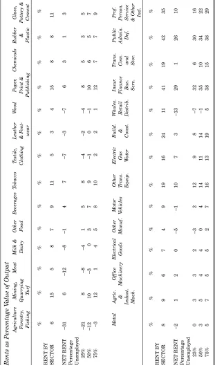
The next issue is to measure labour market rents. I use the difference between the hourly wage in any sector and the lowest hourly wage as a measure of rents (the agricultural sector hourly wages were incredibly low at about thirty pence so I used the next lowest wage which was from wholesale and retail trade as the wage in Agriculture also). If R is the column vector of rents per hour in each sector then R'L gives a vector of rents generated in the economy from an increase in the demand of a pound in any sector. (The R'L vector is the Rent by Sector row of Table 1.)

The R'L vector overestimates rents generated from the expansion of one sector for a number of reasons. As argued above a substantial part (and some argue all) differences in gross wages reflect differences in worker and job characteristics. Additionally, the way we measure rents implicitly assumes that when hours worked increases in any sector the worker had not been earning rents in some other sector. One response to this is to assume that when employment expands in any sector the workers come proportionately from all sectors. We take an employment weighted average of rents in each sector and subtract it from the vector of rents to get (R–A) and then generate (R–A)'L. (The vector (R–A)'L corresponds to the Net Rents row of Table 1.)

T

able 1:

Rent by Sector

(Different fractions of workers coming from unemployment)

Rents as Percentage V

alue of Output

Agriculture Mining, Meat Milk & Other Beverages T obacco T extile, Leather W ood Paper , Chemicals Rubber Glass, Forestry , Quarrying Dairy Food Clothing & Foot-Print & & Pottery & Fishing T urf wear Publishing Plastic Cement % % % % % % % %%%% % % %

RENT BY SECTOR

6 1 5 5 8 7 9 1 1 5 3 4 15 8 8 1 1 NET RENT –31 6 –12 –8 –1 4 7 –7 –3 –7 6 3 1 3 Percentage Unemployed 25% –21 8 – 8 – 4 1 5 8 –4 –2 –4 8 5 3 5 50% –12 10 –3 0 3 7 9 –1 0 – 1 1 0 6 5 7 75% –3 12 1 4 5 8 10 2 2 1 12 7 7 9 Metal Agric. Office Electrical Other Motor Other Electric Build. Wholes. Insur . T rans. Public Prof. & M achinery Goods Manuf. V ehicles T rans. Gas & Retail Finance Com. Admin. Person. Indust. Equip. W ater Const. Distrib. Bus. and Def. Service Mach. Serv . Stor . & Other Ind. % % % % %% % % % %%% % %

RENT BY SECTOR

T

able 2:

Summary Labour Market V

ariables (By Sector)

Agriculture Mining, Meat Milk & Other Beverages T obacco T extile, Leather W ood Paper , Chemicals Rubber Glass, Forestry , Quarrying Dairy Food Clothing & Foot-Print & & Pottery & Fishing T urf wear Publishing Plastic Cement Hourly W age 3.62 7.15 4.71 6.31 5.59 8.47 9.31 4.32 4.61 4.26 6.87 7.62 5.79 6.61 Usual Hours 61.70 47.58 40.00 46.43 41.34 45.20 39.75 37.97 37.15 41.60 41.75 44.08 40.22 42.13

Output per hour

8.14 29.02 90.07 1 12.14 58.12 68.91 53.67 18.03 33.53 23.10 26.06 78.88 29.49 36.34

Unit Labour cost

0.04 0.25 0.05 0.06 0.10 0.12 0.17 0.24 0.14 0.18 0.26 0.10 0.20 0.18 Metal Agric. Office Electrical Other Motor Other Electric Build. Wholes. Insur . T rans. Public Prof. & M achinery Goods Manuf. V ehicles T rans. Gas & Retail Finance Com. Admin. Person. Indust. Equip. W ater Const. Distrib. Bus. and Def. Service Mach. Serv . Stor . & Other Ind. Hourly W age 4.95 5.60 6.34 5.58 4.46 5.43 7.72 7.37 6.20 3.62 1 1.52 5.12 9.64 6.30 Usual Hours 42.73 40.83 40.89 40.33 40.98 43.45 44.33 42.05 42.80 42.90 42.90 41.70 38.90 36.30

Output per hour

23.63 27.51 80.42 41.29 24.19 20.23 23.25 33.79 22.29 10.94 33.39 18.04 16.61 14.41

Unit Labour cost

The Net Rents calculated above could be seen as being appropriate in an economy at full employment where there is no net employment growth. The Gross rents measure assumes all newly employed workers get our estimate of the outside option and might be relevant if there is high unemployment or perfect labour mobility and we are happy to have immigrants take employment. This issue of what the appropriate shadow cost for labour is in the context of project evaluation of industrial projects by the Industrial agencies is discussed in Honohan (1996), McKeon (1980) and Ruane (1980) .

Table 3 below taken from McKeon gives the recruitment patterns of grant-aided industry in 1980. Based on this table over half the employees who were recruited to grant-aided industries had not previously been employed in the Irish economy (of course that is not to say though that a school leaver who got a job in a grant-aided industry would not have found some other job. Much of the literature on wage differentials and labour market rents associate high skill jobs as the high rent jobs. High skill groups are likely to be underrepresented in the unemployed pool. If jobs are created in a high rent sector it is less likely that unemployed workers will get these jobs. One simple way to respond to the issue of where workers come from when a sector expands and whether they had previously been earning rents is to think of it in terms of the fraction of the additional hours work which would go to previously unemployed workers. Say P is the fraction of new hours worked in any sector which would go to previously unemployed (or zero rent) workers and (1–P) is the fraction going to workers from a weighted average of all sectors. In this case if there is a vector of these fractions across sectors (R – (1–P)A)'L is the vector of rents per pound of output in each sector (this corresponds to the last three rows in Table 1 where P the percentage of workers who had been unemployed is assumed to be the same across sectors).

Table 3: Recruitment Patterns for Grant-Aided Industry

Source School Live Manufacturing Agriculture Other Returned

House-Leavers Register Emigrants wives

& AnCO

% 23.3 18.4 24.1 4.9 17 3.6 8.7

Source: McKeon p. 12.

IV DATA

Force Survey, the Census of Industrial Production and the quarterly series of Earnings and Hours Worked issued by the CSO. Appendix 1 lists the sectors used and how they correspond with the Labour Force Survey and Census of Industrial Production.

For Non-Manufacturing sectors the Labour Force Survey was used for hours and employment and the hourly wage by sector was generated as wages and salaries from the input-output tables divided by total hours worked. Hours worked per unit of output was generated as total hours divided by output from the input-output tables. Some sectors (service sectors in particular) had to be aggregated to the sectoral levels given in the Labour Force Survey. Also the Labour Force survey data on hours worked by sector is more aggregated than the employment data so when it was necessary I assumed the same hours worked across sectors where this aggregation took place.

For Manufacturing sectors, the Census of Industrial Production and the series on Hours and Earnings are more disaggregated than the Labour Force Survey. The series on Hours and Earnings was the source for usual hours worked and the Census of Industrial Production for employment. The Census of Industrial Production has a narrower scope than the Labour Force Survey, (it only counts establishments with three or more people for example). However, in the analysis I use hours worked per unit of output and the hourly wage by sector. Since the Census of Industrial Production gives a measure of total output in each sector, as long as I calculate hours per unit of output and hourly wages entirely from data in the Census of Industrial Production and the series on hours and earnings, hopefully I will overcome any bias from using the Labour Force Survey for some sectors and the Census of Industrial Production for others.

Comparing the hourly wage in Table 2 with Rent by Sector in Table 1 we see that accounting for linkages across sectors as we do in Table 1 makes a significant difference to what look like the good and bad industries. For example, Beverages and Tobacco are high wage industries in Table 2 yet when we account for the labour input across sectors rents are not that high in Table 1. A surprising feature of the results is the high wages in many service sectors. The Insurance, Finance and Business Services category possibly contains a lot of high skill and professional workers. Professional Services, Other Industries and Personal Services are aggregated into one sector because of data limitations. This sector contains very different kinds of workers including educational workers, professionals and laundry workers, so we need to be careful about interpreting the results. In some sectors such as Mining or Building and Construction we should clearly be wary that wage differentials reflect compensating differentials. Public Administration is clearly also a special case.

Table 3 we might alternatively allow 50 per cent of workers to come from unemployment. Manufacturing sectors do not have particularly high rents and indeed some sectors have negative rents. Given that as argued rents are probably significantly overstated in gross wage differentials there is no evidence here to support subsidising Manufacturing. If anything some of the service sectors generate the highest rents but given the degree of aggregation and that skill factors might be particularly important in some of these sectors we should be cautious about inferring too much from this.

V CONCLUSION

Sweeny (1992) provides a Table summarising the European Commission’s second survey of state aids. The survey shows aids to manufacturing represented 6.2 per cent of value added between 1986/88. The evidence in this paper suggests that there is not a strong case for continuing subsidies to manufacturing based on the labour markets rents generated.

The notion that output is more responsive to subsidies in some sectors than others, as outlined in Honohan (1996) might be one rationale for subsidising some sectors. The idea is that the industrial development agencies act like discriminating monopolists in setting the grant level in different projects. The results of the theoretical model outlined, do not support the idea that this argument can be used to justify different tax rates for manufacturing and traded services. When we account for the linkages across sectors the empirical analysis discounts any argument that subsidising the traded sector will provide better jobs. Given these results the move towards tax harmonisation across sectors seems like a good idea.

REFERENCES

BARRY, FRANK, 1997. “Dangers for Ireland of an EMU Without the UK: Some Calibration Results”, The Economic and Social Review, Vol. 28, No. 4, pp. 333-349. BARRY, FRANK, and AOIFE HANNAN, 1995. “Multinationals and Indigenous

Employ-ment: An Irish Disease?” UCD Economics Department Working Paper WP95/13. BULOW, JEREMY, and LAWRENCE H. SUMMERS, 1986. “A Theory of Dual Labor

Markets with Applications to Industrial Policy, Discrimination and Keynesian Unemployment”, Journal of Labor Economics.

CENTRAL STATISTICS OFFICE, 1990. Input-Output Tables for 1990, Dublin: Stationery Office.

CENTRAL STATISTICS OFFICE, 1990. Census of Industrial Production 1990, Dublin: Stationery Office.

CENTRAL STATISTICS OFFICE, 1990. Labour Force Survey 1990, Dublin: Stationery Office.

DENNY, KEVIN, AOIFE HANNAN, and KEVIN O’ROURKE, 1995. “Harmonizing Irish Tax Rates: A Computable General Equilibrium Approach”, UCD Economics Department Working Paper WP95/3.

DICKENS, WILLIAM T., 1995. “Do Labor Rents Justify Strategic Trade and Industrial Policy”, NBER Working Paper Number 5137.

HENRY, E.W., 1986. Multisector Modelling of the Irish Economy, With Special Reference to Employment Projections, General Research Series Paper No. 128, Dublin: The Economic and Social Research Institute.

HONOHAN, PATRICK, 1996. “Methodological Issues in Evaluation of Irish Industrial Policy”, The Economic and Social Research Institute Working Paper 69.

KATZ, LAWRENCE F., and LAWRENCE H. SUMMERS, 1989. Industry Rents: Evidence and Implications, Brookings Papers on Economic Activity, Microeconomics.

McKEON, JOHN, 1980. “Economic Appraisal of Industrial Projects in Ireland”, Journal of the Statistical and Social Inquiry Society of Ireland, pp. 119-143.

NATIONAL ECONOMIC AND SOCIAL COUNCIL, 1990. A Strategy for the Nineties: Economic Stability and Structural Change, NESC Report Number 89, Dublin: Stationery Office.

O’MALLEY, EOIN, 1995. An Analysis of Secondary Employment Associated With Manufacturing Industry, General Research Series Paper No. 167, Dublin: The Economic and Social Research Institute.

O’ROURKE, KEVIN, 1994. “Industrial Policy, Employment Policy and the Non-Traded Sector”, Journal of the Statistical and Social Inquiry Society of Ireland, Vol. XXVII, Part II.

RUANE, FRANCES, 1980. “Optimal Labour Subsidies and Industrial Development in Ireland”, The Economic and Social Review, Vol. 11, No. 2, pp. 77-98.

SWEENY, PAUL, 1992. “Symposium on the Findings of the Industrial Policy Review Group”, Journal of the Statistical and Social Inquiry Society of Ireland, pp. 119-143. WALSH, FRANK, 1994. “The Effect of Labour Market Subsidies in the Presence of

Efficiency Wages”, Unpublished.

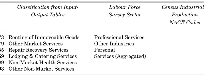
APPENDIX 1: Industry Classifications

Classification from Input- Labour Force Census Industrial

Output Tables Survey Sector Production

NACE Codes

01 Agriculture, Forestry and Agriculture, Forestry

Fishing and Fishing

03 Coal/Lignite Briquettes Mining, Quarrying

and Turf Production 05 Products of Coking

07 Petrol Products/Nat. Gas 11 Radioactive material & Ores 13 Metals and Ores

09 Electricity/Gas/Water 13, 16 & 17

APPENDIX 1 (Cont’d): Industry Classifications

Classification from Input- Labour Force Census Industrial

Output Tables Survey Sector Production

NACE Codes

17 Chemical Products 25-26

19 Metal products excl. Machinery

& Transport Equipment 31

21 Agric./Industrial Machinery 32

23 Office Machines 33 & 37

25 Electrical Goods 34

27 Motor Vehicles 35

29 Other Transport Equipment 36

31 Meat/Meat Products 412

33 Milk & Dairy Products 413

35 Other Food Products 416, 422, 419,

420-421, 411, 414, 415, 417-418, 423

37 Beverages 424-428

39 Tobacco Products 429

41 Textiles/Clothing 43 & 453-456

43 Leather/Footwear 44, 451

45 Wooden Products/Furniture 46

47 Paper Printing Products 47

49 Rubber & Plastic Products 481-483

51 Other Manufacturing 49

53 Building & Construction Building & Construction

57 Wholesale & Retail Trade Wholesale Distribution Retail Distribution (Aggregated)

69 Credit & Insurance Insurance, Finance and

71 Business Services Business Services

61 Inland Transport Transport,

Communi-63 Maritime/Air transport cations and

65 Auxillary Transport Storage

67 Communication Services

81 General Public Services Public Administration

APPENDIX 1 (Cont’d): Industry Classifications

Classification from Input- Labour Force Census Industrial

Output Tables Survey Sector Production

NACE Codes

73 Renting of Immoveable Goods Professional Services

79 Other Market Services Other Industries

55 Repair Recovery Services Personal

59 Lodging & Catering Services Services (Aggregated) 89 Non-Market Health Services

93 Other Non-Market Services

The first column gives the input-output sector. If there is more than one I/O sector in a row they were aggregated to make them consistent with labour market Data. The corresponding labour market Data came from the Labour Force Survey if there is an entry in the second Column or the Census of Industrial Production and Quarterly Series of Hours and Earnings if there is an entry in the third column. LFS industry classifications are based on those used in the 1986 Census.

APPENDIX 2: Simulations of Sufficient Conditions

Table A2.1: TRUE Indicates sufficient conditions for subsidising

non-tradeables being cheaper hold

supply elasticity 0.1

εnt

εtn 0.1 0.2 0.3 0.4 0.5 0.6 0.7 0.8 0.9

0.1 FALSE FALSE FALSE FALSE FALSE FALSE FALSE FALSE FALSE

0.2 FALSE FALSE FALSE FALSE FALSE TRUE TRUE TRUE TRUE

0.3 FALSE FALSE FALSE TRUE TRUE TRUE TRUE TRUE TRUE

0.4 FALSE FALSE TRUE TRUE TRUE TRUE TRUE TRUE TRUE

0.5 FALSE FALSE TRUE TRUE TRUE TRUE TRUE TRUE TRUE

0.6 FALSE TRUE TRUE TRUE TRUE TRUE TRUE TRUE TRUE

0.7 FALSE TRUE TRUE TRUE TRUE TRUE TRUE TRUE TRUE

0.8 FALSE TRUE TRUE TRUE TRUE TRUE TRUE TRUE TRUE

0.9 FALSE TRUE TRUE TRUE TRUE TRUE TRUE TRUE TRUE

Table A2.2: TRUE Indicates sufficient conditions for subsidising

non-tradeables being cheaper hold

supply elasticity 0.5

εnt

εtn 0.1 0.2 0.3 0.4 0.5 0.6 0.7 0.8 0.9

0.1 FALSE FALSE FALSE FALSE FALSE FALSE FALSE FALSE FALSE

0.2 FALSE FALSE FALSE FALSE FALSE FALSE FALSE FALSE FALSE

0.3 FALSE FALSE FALSE FALSE FALSE FALSE FALSE FALSE FALSE

0.4 FALSE FALSE FALSE FALSE FALSE FALSE FALSE FALSE FALSE

0.5 FALSE FALSE FALSE FALSE FALSE FALSE FALSE FALSE FALSE

0.6 FALSE FALSE FALSE FALSE FALSE FALSE FALSE FALSE TRUE

0.7 FALSE FALSE FALSE FALSE FALSE FALSE FALSE TRUE TRUE

0.8 FALSE FALSE FALSE FALSE FALSE FALSE TRUE TRUE TRUE

0.9 FALSE FALSE FALSE FALSE FALSE TRUE TRUE TRUE TRUE

1 FALSE FALSE FALSE FALSE FALSE TRUE TRUE TRUE TRUE

Table A2.3: TRUE indicates sufficient conditions for subsidising tradeables

being cheaper hold

supply elasticity 1

εnt

εtn 1.1 1.2 1.3 1.4 1.5 1.6 1.7 1.8 1.9

0.1 TRUE TRUE TRUE TRUE TRUE TRUE TRUE TRUE TRUE

0.2 TRUE TRUE TRUE TRUE TRUE TRUE TRUE TRUE TRUE

0.3 TRUE TRUE TRUE TRUE TRUE TRUE TRUE TRUE TRUE

0.4 TRUE TRUE TRUE TRUE TRUE TRUE TRUE TRUE TRUE

0.5 TRUE TRUE TRUE TRUE TRUE TRUE TRUE TRUE TRUE

0.6 TRUE TRUE TRUE TRUE TRUE TRUE FALSE FALSE FALSE

0.7 TRUE TRUE TRUE TRUE FALSE FALSE FALSE FALSE FALSE

0.8 TRUE TRUE FALSE FALSE FALSE FALSE FALSE FALSE FALSE

0.9 TRUE FALSE FALSE FALSE FALSE FALSE FALSE FALSE FALSE