On Solving Unsymmetric Tridiagonal Systems
Without Interchanges
Jennifer B. Erway,
∗Roummel F. Marcia,
†and Joseph A. Tyson,
∗Abstract— It has been shown recently that a non-singular tridiagonal linear system of the formT x=b can be solved in a backward-stable manner using the LBMTdecomposition, i.e., T = LBMT, where L and M are unit lower triangular matrices and B is block diagonal with 1×1 and 2×2 blocks. In this pa-per, we demonstrate the robustness of two algorithms that compute a backward-stable LBMT decomposi-tion using a wide range of well-condidecomposi-tioned and ill-conditioned linear systems. Numerical results suggest that these algorithms are comparable to Gaussian elimination with partial pivoting (GEPP). However, unlike GEPP, these algorithms do not require row interchanges, and thus, may be used in applications where row interchanges are not possible. In addition, substantial computational savings can be achieved by carefully managing the nonzero elements of the fac-torsL, B, and M.
Keywords: linear algebra, tridiagonal systems, diago-nal pivoting, Gaussian elimination
1
Introduction
A nonsingular tridiagonal linear system of the form
T x=b, (1)
whereT ∈IRn×n andxand b∈IRn, is often solved us-ing matrix factorizations. IfT is symmetric and positive definite, then the Cholesky decomposition or the LDLT factorization, where L is a lower triangular matrix and
D is a diagonal matrix, can be used to solve (1). IfT is symmetric but indefinite, then with row and/or column permutations, the LBLTfactorization can be used, where
B is block diagonal with either 1×1 or 2×2 blocks (see e.g., [2, 3, 4, 5, 6, 9]). Finally, if T is unsymmet-ric, then (1) can be solved using Gaussian elimination with full pivoting or with partial pivoting (GEPP). Re-cent work by the authors [8] shows that (1) can be solved in a backward-stable manner using the LBMT decompo-sition ofT, i.e.,T =LBMT, where Bis a block diagonal
∗Department of Mathematics, Wake Forest University, Winston-Salem, NC 27106, USA. J. B. Erway and J. A. Tyson are supported by the National Science Foundation grant DMS-0811106
†School of Natural Sciences, 5200 North Lake Road, University of California, Merced, Merced, CA 95343. Tel: 209-228-4874. Fax: 209-228-4060. Email: [email protected]. R. F. Marcia is sup-ported by the National Science Foundation grant DMS-0811062
matrix with either 1×1 or 2×2 blocks andLandM are unit-lower tridiagonal matrices.
In this paper, we examine two algorithms presented in [8] for forming a backward-stable LBMTdecomposition of a nonsingular tridiagonal matrix T. We demonstrate that the resulting L, B, and M factors from either al-gorithm can be used to solve the linear systemT x =b
with accuracy comparable to Gaussian eliminiation with partial pivoting (GEPP). However, unlike GEPP, nei-ther algorithm requires row interchanges, making them particularly useful in look-ahead Lanczos methods [11] and composite-step bi-conjugate gradient methods [1] for solving unsymmetric linear systems.
2
Diagonal pivoting
LetT ∈IRn×ndenote the unsymmetric nonsingular tridi-agonal matrix T = ⎡ ⎢ ⎢ ⎢ ⎢ ⎢ ⎢ ⎢ ⎣
α1 γ2 0 · · · 0
β2 α2 γ3 . .. ...
0 β3 α3 . .. 0 ..
. . .. ... ... γn 0 · · · 0 βn αn
⎤ ⎥ ⎥ ⎥ ⎥ ⎥ ⎥ ⎥ ⎦ . (2)
We partitionT in the following manner:
T =
d n−d d
n−d
B1 T12T
T21 T22
The computation of the LBMTfactorization, whereLand
M are unit lower triangular andBis block diagonal with 1×1 and 2×2 blocks, involves choosing the dimension (d= 1 or 2) of the pivotB1 at each stage:
T =
Id 0
T21B1−1 In−d
B1 0
0 Sd
Id B−11T12T 0 In−d ,
(3)
factorization can be defined recursively. Specifically, for
d= 1,
S1=T22−β2γ2
α1 e (n−1)
1 e(1n−1)T,
wheree(1n−1) is the first column of the (n−1)×(n−1) identity matrix. Ford= 2,
S2=T22−
α1β3γ3
Δ
e(1n−2)e(1n−2)T.
where
Δ=α1α2−β2γ2
is the determinant of the 2×2 pivot B1 and e(1n−2) is the first column of the (n−2)×(n−2) identity matrix. In both cases Sd and T22 differ only in the (1,1) entry; thus, the LBMTfactorization can be recursively defined to obtain the matricesL,B, and M.
The algorithms in [8] can be completely described by looking at the first stage of the factorization.
2.1
Algorithm I
Let
L1=T21B1−1 and M1T =B−11T12T
in (3). If a 1×1 pivot is used, then the (1,1) elements of
L1and M1 are
(L1)1,1= β2
α1 and (M1)1,1=
γ2
α1. (4)
If a 2×2 pivot is used, then the (1,1) and (1,2) elements ofL1and M1 are
(L1)1,1 = −β2β3
Δ , (M1)1,1 = − γ2γ3
Δ ,
(L1)1,2 = α1β3
Δ , (M1)1,2 =
α1γ3
Δ .
(5)
With elements ofL1 and M1 for a 2×2 pivot scaled by the constantκ(described below) from the Bunch pivoting strategy [2], Algorithm I chooses a 1×1 pivot if the both of the entries in (4) is smaller than the largest entry in (5) in magnitude, i.e.,
max
|β2|
|α1|,
|γ2|
|α1|
≤maxκ
|β2β3|
|Δ| ,
|α1β3|
|Δ| ,
|γ2γ3|
|Δ| ,
|α1γ3|
|Δ|
,
(6)
and a 2×2 pivot is chosen otherwise. In other words, Algorithm I chooses pivot sizes based on whichever leads to smaller entries (in magintude) in the computed factors
LandM. In addition, we impose the criterion that if
|α1α2| ≥κ|β2γ2|, (7)
a 1×1 pivot is chosen. This additional criterion guaran-tees that ifT is positive definite, the LBMTfactorization
reduces to the LDMTfactorization. The choice of pivot size in the first iteration is described as follows:
Algorithm I.This algorithm determines the size of the pivot for the first stage of the LBMTfactorization applied to a tridiagonal matrixT ∈IRn×n.
κ= (√5−1)/2≈0.62
Δ=α1α2−β2γ2
if |α1α2| ≥κ|β2γ2| or |Δ|max{|β2|,|γ2|} ≤
κ|α1|max{|β2β3|,|α1β3|,|γ2γ3|,|α1, γ3|}
dI = 1 else
dI = 2 end
The choice ofκ, which is a root of the equationκ2+κ−1 = 0, balances the element growth in the Schur complement for both pivot sizes by equating the maximal element growth (see [2] for details). A recursive application of Algorithm I yields a factorizationT =LBMT, whereL
andM are unit lower triangular andBis block diagonal. (In fact, one can show thatLandM are such thatLi,j=
Mi,j = 0 fori−j >2.) Intuitively, Algorithm I chooses a 1×1 pivot if α1 is sufficiently large relative to the determinant of the 2×2 pivot, i.e., a 1×1 pivot is chosen if a 2×2 pivot is relatively closer to being singular than
α1 is to zero.
2.2
Algorithm II
We also proposed an alternative pivoting strategy that is based on the strategy of Bunch and Kaufman for sym-metrictridiagonal matrices (Section 4.2, [3]). (Note that this strategy is different from their well-known symmetric factorization using partial pivoting.) This second strat-egy chooses a 1×1 pivot if the (1,1) diagonal entry is sufficiently large relative to the off-diagonals, i.e.,
|α1|σ1≥κ|β2γ2|,
where
σ1= max{|α2|,|γ2|,|β2|,|γ3|,|β3|},
andκis as in Sec. 2.1. This algorithm can be completely described in the first step:
Algorithm II. This alternative algorithm determines the size of the pivot for the first stage of the LBMT fac-torization applied to a tridiagonal matrixT ∈IRn×n.
κ= (√5−1)/2≈0.62
σ1= max{|α2|,|γ2|,|β2|,|γ3|,|β3|}
if |α1|σ1≥κ|β2γ2|,
else
dII = 2 end
It can be shown that Algorithms I and II are very related in that whenever Algorithm I chooses a 1×1 pivot, so does Algorithm II. In fact, the only difference between the two algorithms is that on occasion, Algorithm I may choose a 2×2 pivot while Algorithm II chooses two consecutive 1×1 pivots.
2.3
Backward stability result
These two pivoting strategies imply a backward stabil-ity result which demonstrates that (a) the difference be-tween computed factorization LBMT and the original tridiagonal matrixT is small (i.e., it is of order machine precision), and (b) the computed solutionxis the exact solution to a nearby problem. More formally, we state the following theorem:
Theorem 1. Assume the LBMTfactorization of the un-symmetric tridiagonal matrixT ∈IRn×n obtained using the pivoting strategy of Algorithm I or II yields the com-puted factorization T ≈LBMT, and let xbe the com-puted solution toT x=bobtained using the factorization. Assume that all linear systems Ey = f involving 2×2 pivotsE are solved using the explicit inverse. Then
T−LBMT =ΔT1, and (T+ΔT2)x=b,
where
ΔTimax≤cuTmax+O(u2), i= 1,2,
wherecis a constant anduis the machine precision.
Proof. See [8].
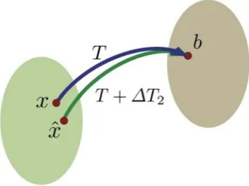
Pictorially, the backward stability result of Theorem 1 is represented in Fig. 1.
In addition to computing a backward-stable LBMT de-composition ofT, these algorithms have minimal storage requirements. Specifically,T is tridiagonal, and thus, can stored using three vectors. Moreover, updating the Schur complement requires updating only one nonzero compo-nent of T. The matrices Land M are unit-lower trian-gular with Li,j = Mi,j = 0 for i−j > 2; thus, their entries can be stored in two vectors each. Finally, B is block-diagonal with 1×1 or 2×2 blocks, requiring only three vectors for storage.
3
Numerical experiments
Numerical tests were run usingMatlabimplementations
of Algorithm I, Algorithm II, GEPP, and the Matlab
[image:3.595.329.510.101.236.2]backslash command (“\”). (Specifically, Algorithm I and Algorithm II were embedded in a code that used one for-ward substitution to solve withL, one back substitution
Figure 1: Theorem 1 implies not only that the product of the computed factorsLbBbMcT is very close to the original matrix T, but that the computed solution ˆxis the exact solution to a nearby problem, i.e., the components ofΔT2 are very small.
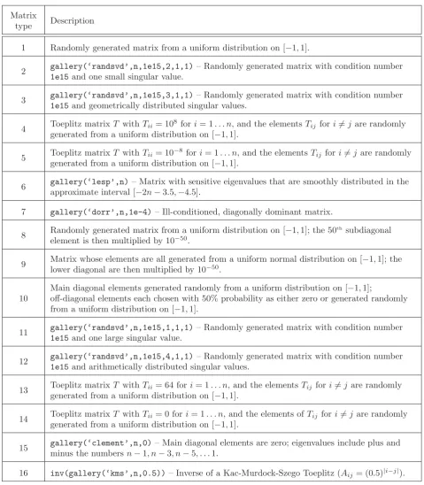
to solve with MT, and a solve with the block-diagonal factor B). We compared the performance of each code on 16 types of nonsingular tridiagonal linear systems of the formT x=b. The test set of system matrices contains a wide range of difficulty. Many ill-conditioned matrices were chosen as part of the test set in order to compare algorithm robustness. (Ill-conditioned matrices are of-ten challenging for matrix-factorization algorithms.) The test set of system matrices was taken from recent liter-ature (specifically, [7] and [10]) on estimating condition numbers of ill-conditioned matrices–a task that can be-come increasingly difficult the more ill-conditioned the matrix is.
Table 1 contains a description of each tridiagonal ma-trix type in the test set. The first ten mama-trix types listed are based on test cases in [10]. Types 11-14 correspond to test cases found in [7] not found in [10], i.e., we eliminated redundant types. Finally, we include two additional tridi-agonal matrices (Types 15-16) that can be generated us-ing the Matlab command gallery. For our tests, T
was chosen to be a 100×100 matrix. The elements ofb
were chosen from a uniform distribution on [−1,1].
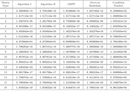
One system matrix was generated from each matrix type, and together with a vector b, the same linear system of the formT x=b was solved by each algorithm. Table 2 shows the relative errors associated with each method. Columns 2-5 of the table contain the relative error
Txˆ−b2
b2 ,
Table 2 suggests that all four algorithms are comparable on a wide variety of linear systems. When the system matrix is well-conditioned (e.g., Types 1, 4, 6, 8, 10, 13, 14, 16), the algorithms have relative errors that are close to machine precision and that are comparable to one an-other. On the other hand, more significant differences occur when the system matrix is very ill-conditioned. For Type 5, the Algorithms I and II perform particu-larly poorly, and the solutions are offered by GEPP and theMatlabbackslash command are also very poor, with
an error near 1016. In fact, due to the ill-conditioning of the system matrix, all methods failed to solve the linear system. Finally, for Types 2, 3, 7, 9, 11, 12, and 15, the system matrices are ill-conditioned, however all the meth-ods obtain relative errors within an order of magnitude of each other.
4
Conclusions and future work
Algorithms I and II, proposed in [8], were shown to com-pute a backward-stable LBMTdecomposition of any non-singular tridiagonal matrix. Numerical results on a wide range of linear systems suggest that the performance of Algorithms I and II are comparable to GEPP and the
Matlab backslash command.
Future work will focus on embedding Algorithm I and II into methods such as the look-ahead Lanczos meth-ods and composite-step bi-conjugate gradient methmeth-ods for solving unsymmetric linear systems.
References
[1] R. E. Bank and T. F. Chan,A composite step bi-conjugate gradient algorithm for nonsymmetric lin-ear systems, Numer. Algorithms, 7, pp. 1–16, 1994.
[2] J. R. Bunch, Partial pivoting strategies for sym-metric matrices, SIAM J. Numer. Anal., 11, pp. 521– 528, 1974.
[3] J. R. Bunch and L. Kaufman,Some stable meth-ods for calculating inertia and solving symmetric lin-ear systems, Math. Comp., 31, pp. 163–179, 1977.
[4] J. R. Bunch and R. F. Marcia,A pivoting strat-egy for symmetric tridiagonal matrices, Numer. Lin-ear Algebra Appl., 12, pp. 911–922, 2005.
[5] , A simplified pivoting strategy for symmetric tridiagonal matrices, Numer. Linear Algebra Appl., 13, pp. 865–867, 2006.
[6] J. R. Bunch and B. N. Parlett, Direct meth-ods for solving symmetric indefinite systems of linear equations, SIAM J. Numer. Anal., 8, pp. 639–655, 1971.
[7] I. S. Dhillon,Reliable computation of the condition number of a tridiagonal matrix in O(n)time, SIAM J. Matrix Anal. Appl., 19 (1998), pp. 776-796.
[8] J. B. Erway and R. F. Marcia,A backward sta-bility analysis of diagonal pivoting methods for solv-ing unsymmetric tridiagonal systems without inter-changes. Accepted for publication in Numerical Lin-ear Algebra with Applications.
[9] H. R. Fang and D. P. O’Leary,Stable factoriza-tions of symmetric tridiagonal and triadic matrices, SIAM Journal on Matrix Analysis and Applications, 28, pp. 576–595, 2006.
[10] G. I. Hargreaves,Computing the Condition Num-ber of Tridiagonal and Diagonal-Plus-Semiseparable Matrices in Linear Time, Numerical Analysis Re-port 447, Manchester Centre for Computational Mathematics, Manchester, 2004.
Table 1: Tridiagonal matrix types used in the numerical experiments
Matrix
type Description
1 Randomly generated matrix from a uniform distribution on [−1,1].
2 gallery(‘randsvd’,n,1e15,2,1,1)– Randomly generated matrix with condition number
1e15and one small singular value.
3 gallery(‘randsvd’,n,1e15,3,1,1)– Randomly generated matrix with condition number
1e15and geometrically distributed singular values.
4 Toeplitz matrixT withTii = 108 fori= 1. . . n, and the elementsTij fori=j are randomly generated from a uniform distribution on [−1,1].
5 Toeplitz matrixT withTii = 10−8fori= 1. . . n, and the elementsTij fori=j are randomly generated from a uniform distribution on [−1,1].
6 gallery(‘lesp’,n)– Matrix with sensitive eigenvalues that are smoothly distributed in the approximate interval [−2n−3.5,−4.5].
7 gallery(‘dorr’,n,1e-4)– Ill-conditioned, diagonally dominant matrix.
8 Randomly generated matrix from a uniform distribution on [−1,1]; the 50
thsubdiagonal
element is then multiplied by 10−50.
9 Matrix whose elements are all generated from a uniform normal distribution on [−1,1]; the lower diagonal are then multiplied by 10−50.
10
Main diagonal elements generated randomly from a uniform distribution on [−1,1];
off-diagonal elements each chosen with 50% probability as either zero or generated randomly from a uniform distribution on [−1,1].
11 gallery(‘randsvd’,n,1e15,1,1,1)– Randomly generated matrix with condition number
1e15and one large singular value.
12 gallery(‘randsvd’,n,1e15,4,1,1)– Randomly generated matrix with condition number
1e15and arithmetically distributed singular values.
13 Toeplitz matrixT withTii = 64 fori= 1. . . n, and the elementsTij fori=j are randomly generated from a uniform distribution on [−1,1].
14 Toeplitz matrixT withTii = 0 fori= 1. . . n, and the elements ofTij fori=j are randomly generated from a uniform distribution on [−1,1].
15 gallery(‘clement’,n,0)– Main diagonal elements are zero; eigenvalues include plus and minus the numbersn−1, n−3, n−5, . . .1.
Table 2: Relative errors for four methods for solving the tridiagonal systemT x=b.
Matrix
Type Algorithm I Algorithm II GEPP
Matlab
Backslash
Condition Number
1 3.358363e-15 2.759199e-15 1.815859e-15 1.837180e-15 6.329660e+02
2 1.517113e-03 1.517113e-03 1.517113e-03 1.517113e-03 1.068959e+15
3 1.422747e-05 2.261760e-05 8.733909e-06 6.084902e-06 1.002161e+15
4 9.931598e-17 9.931598e-17 8.106222e-17 8.106222e-17 1.000000e+00
5 3.932643e+23 3.932643e+23 1.302276e+16 1.302276e+16 1.570243e+41
6 1.513163e-16 1.513163e-16 1.357171e-16 1.357171e-16 6.748520e+01
7 4.472943e+01 4.472943e+01 6.609908e+01 6.609908e+01 2.784168e+16
8 1.796253e-15 1.807151e-15 7.290777e-16 1.089269e-15 1.093088e+03
9 2.298240e-10 2.298240e-10 1.307689e-10 1.307689e-10 1.101082e+08
10 3.857912e-14 3.857912e-14 3.017280e-14 3.017259e-14 1.489926e+04
11 5.856221e-05 5.856221e-05 2.155033e-05 2.155033e-05 1.259243e+15
12 3.526433e-03 3.124242e-03 1.539025e-03 1.655561e-03 8.930231e+14
13 8.951786e-17 8.951786e-17 6.956100e-17 6.956100e-17 1.006886e+00
14 1.706070e-14 1.706081e-14 5.410519e-15 5.411247e-15 5.378205e+05
15 2.765054e-02 2.765054e-02 1.212209e-02 1.186110e-02 3.144575e+15